Abstract
Physical dynamic characteristics and control studies were conducted for pneumatic artificial muscle (PAM), the core component of the drive of lower limb rehabilitation robots. Firstly, a static model and a dynamic model of the pneumatic artificial muscle were established. Then a test bench was designed to perform dynamic characteristic test simulations and experiments. After that, the pneumatic artificial muscle test bench was designed to simulate and test its dynamic characteristics. Finally, a typical PID (Proportional Integral Derivative) controller was built to perform control simulations and step control experiments for the pneumatic artificial muscle. Experiments show that the PID can achieve stable and accurate tracking of the signal and meet the application requirements of PAM.
1. Introduction
The pneumatic artificial muscle (PAM) is a pneumatic actuator with biomimetic muscle properties, the original concept of artificial pneumatic muscle was first proposed by McKibben in the 1950s [1]. Because its structure is mainly made of rubber, it has no acceleration break point during the filling and deflating process; this property allows flexible change for pneumatic muscle. Due to the cushioning effect of rubber, pneumatic muscles are widely used in medical assistance. Pneumatic artificial muscles are characterized by an enormous power/mass ratio and high flexibility and can be widely used to drive systems with strongly nonlinear motion characteristics; moreover, their inherent flexibility and limited maximum contraction make them very safe and suitable for rehabilitation applications, such as ankle rehabilitation robots and agricultural picking robots [2,3].
Among them, Li Baoren [4] from Huazhong University of Science and Technology, China, proposed the concept of using this flexible woven actuator system as a pneumatic element and thus put it into the category of pneumatic transmission systems for pneumatic control to build and control this model. They also described the dynamic and static characteristics of the pneumatic artificial muscle system using fluid dynamics and thermodynamics theories. They summarized and proposed that the motion of the pneumatic artificial muscle system can be divided into four processes: the isovolumetric expansion process, the expansion-contraction process, the exhaust extension process and the isovolumetric exhaust process. This segmental approach to the study simplifies the complex pneumatic muscle movements and facilitates modeling pneumatic muscle trajectories. The pneumatic manual muscle is flexible and non-linear, especially when the drive is at low operating pressures and loads. This woven elastic drive is mechanically and mathematically challenging to model accurately. Moreover, because of this non-linearity between pressure and output force, it makes the pneumatic artificial muscle a pneumatic element, and from its emergence to its application, it has gone through a long historical process [5]. In the 1990s, Chou [6] of Harvard University developed an ideal mathematical model of pneumatic artificial muscles based on the energy conservation law combined with the thermodynamic perfect gas equation of state. The scholar Tondu [7] extended the above model and converted it into a new model. However, these two models of pneumatic artificial muscles ignore the effects of friction at the ends of the pneumatic artificial muscles and the elastic change of the material when considering them. Therefore, it leads to a large discrepancy between this ideal model and the actual model. As the application of pneumatic artificial muscles spreads, the research on its modeling has increased. This aspect was investigated by Repperger D W et al. [8], researchers at the U.S. Air Force Laboratory. During the experiment, the pneumatic muscle is equated to a spring, but the stiffness of the equivalent spring can be changed. During the inflation and deflation of pneumatic muscles with different stiffness, a model of pneumatic muscles was fitted by synthesizing a large amount of experimental data. However, due to the other models and manufacturers, each pneumatic muscle requires many experiments to fit the above model before use, which also limits the application of the method. Scholar Tondu [9] has also recently developed a mathematical model of pneumatic artificial muscles containing four parameters, which combines empirical and physical theories to explain the connection between static forces and pressures and the stretchability of pneumatic artificial muscles. However, it is also true that this mathematical model only applies to the new Festo air muscles derived from the common McKibben artificial muscles and cannot be used on a large scale and universally to satisfy the general pneumatic artificial muscles.
PID (Proportional Integral Derivative) control is one of the most classical and widely used control theories in the field of control. Some scholars, Wang Yuzhong et al. [10], applied it to performance prediction and validated it on the temperature thermodynamic model of coke ovens. Scholars Zhao Cheng et al. [11] proposed an explanation to combine PID control with nonlinear systems and used it to establish a three-dimensional closed-loop nonlinear system parameter set to verify the control effectiveness of PID in nonlinear systems. Moreover, scholars Jun Wang et al. [12] designed a new algorithm combining PID control and a hybrid neural network to achieve control speed and accuracy of the hydraulic control system of an unmanned platform. They verified its good control effect on the engine and hydraulic pump in the hydraulic system by simulation and experiment. The above industrial field control for PID is mainly used in thermodynamics, fluid drive, and the neural network, as predictive control is above the application. It will be combined in the pneumatic artificial muscle above the application; the pneumatic artificial muscle combined with the PID control effect and the actual use of demand are not well understood. Hence, a PID control-driven pneumatic artificial muscle has an extremely practical significance and broad market application value.
In addition, there are other studies on control strategies for pneumatic artificial muscles. Scholars Repperger [13] relied on sliding mode control as a control strategy, in which the mathematical model and load changes no longer influence after the joint system enters the sliding region; it also belongs to nonlinear intelligent control with relatively good robustness. Hesselroth [14] used multilayer self-organizing neural networks to control the joint position of artificial pneumatic muscles, which had some control effect but could not eliminate coordinate oscillations. Lilly et al. [15] continuously adjusted the real-time parameters on the host computer by identifying the system parameters online and facing the real-time changing system requirements. Through this continuous change, the system is learning to achieve its target control effect. However, since the pneumatic artificial muscle is a regular repetitive motion, but also a careful consideration of the system’s economy, this control method will not be applied.
In summary, the use of these strategies requires the establishment of a precise mathematical model of the robot joints, which often affects the effectiveness of such control methods when the model parameters or the applied loads change due to the complexity and unknown nature of the internal and external conditions, combined with the excellent suppleness of the pneumatic artificial muscles themselves. In practical applications, the best control strategy for lower limb rehabilitation robots driven by pneumatic artificial muscles is mainly position control. The position control strategy requires high precision and signal stability of the control system. The classical PID controller is mostly used in medium and large industrial fields such as aerospace, hydraulic fluid field, etc., but it is rarely used in medical or rehabilitation areas for the control of pneumatic artificial muscles as drive elements for lower limb rehabilitation robots. Therefore, in this paper, the joints of a lower limb rehabilitation robot are studied, and an adaptive Proportional Integral Derivative (PID) controller is designed for pneumatic artificial muscles driven by high-speed switching valves, the implementation of which does not depend on an accurate mathematical model for pneumatic artificial muscles. To verify the control effect of this PID controller on the pneumatic artificial muscle and the characteristics of the pneumatic artificial muscle itself, this paper uses the model based on the pneumatic artificial muscle model studied by previous researchers, considering the influence of the elastic friction of the end constraint and introducing the correction coefficient to simulate its dynamic characteristics and step signal; moreover, it establishes the test bench of the pneumatic artificial muscle position servo system, and conducts its dynamic characteristics experiment and step tracking test on the test bench, and finally compares and discusses the simulation and its experimental results.
2. Pneumatic Artificial Muscle Modeling and Dynamic Simulation
2.1. Static Model of Pneumatic Artificial Muscles
Defining a mathematical model for pneumatic artificial muscles is the basis of this study on pneumatic muscles, which are mainly composed of rubber and a mesh of woven fiber. The existence of elasticity in rubber and the friction between the woven mesh and rubber tube, as well as the compressibility of the gas volume, lead to a strong non-linearity of the output of pneumatic muscles, making it difficult to establish an accurate mathematical model. Therefore, under the assumption that the shape of the pneumatic artificial muscle is an ideal cylinder after inflation, this static model is obtained according to the law of conservation of energy and the principle of virtual work and by taking into consideration the influence of the curvature of the two ends of the pneumatic artificial muscle on the contraction force and introducing correction coefficients [16]:
where: R0 is the initial state radius of the pneumatic artificial muscle, k0 is the correction parameter, ε is the contraction rate of the pneumatic artificial muscle, , E0 and E1 are the initial state length of the pneumatic artificial muscle and the length at contraction, respectively, p is the internal cavity pressure of pneumatic artificial muscle, A = 3/tan2γ, B = e/sin2γ, γ is the initial state braiding angle of pneumatic artificial muscle.
2.2. Modeling the Dynamic Properties of Pneumatic Artificial Muscles
The pneumatic high-speed switching valve used in this design is controlled by the Pulse Width Modulation (PWM) signal generated by the microcontroller’s digital output. To facilitate the derivation of the dynamic characteristics of the pneumatic muscle system, the following assumptions are made for the design; moreover, the pneumatic artificial muscle model control schematic is shown in Figure 1:
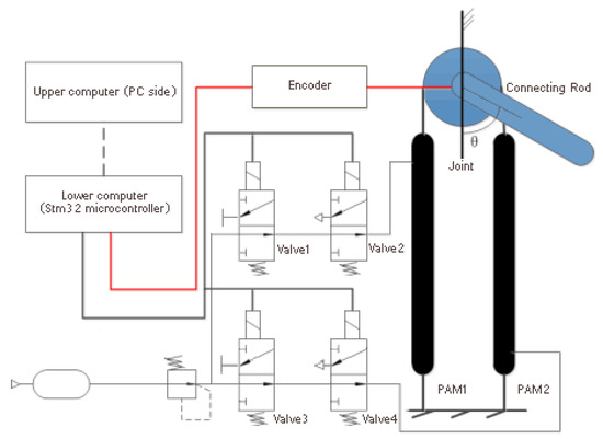
Figure 1.
Control principle diagram of pneumatic artificial muscle model.
(1) The gas is ideal;
(2) There is no leakage of pneumatic components;
(3) The pneumatic muscle filling and deflating process are adiabatic processes;
(4) The thermodynamic process of the gas inside the pneumatic muscle chamber is quasi-static;
(5) The gas source pressure, ambient pressure and ambient temperature are stable.
Inside the high-speed switching valve, the gas is subjected to various influences during its motion, and thus its mass flow rate is calculated using the Sanvile formula [17], which is given by:
where Qg is the gas mass flow rate, u is the input pulse width modulation signal duty cycle, S is the effective cross-sectional area of the valve port circulation, R1 is the critical pressure ratio, p1 and p2 are the upstream and downstream pressures, respectively, T is the gas source temperature, K is the adiabatic gas index, and C is the gas constant.
The flow of gas inside the chamber of pneumatic artificial muscle obeys the law of thermodynamics and the rule of energy conservation, according to which the energy conservation equation of pneumatic artificial muscle can be obtained as follows:
where p is the pneumatic muscle chamber pressure and V is the chamber volume during pneumatic muscle contraction.
For pneumatic artificial muscles, there are:
where e is the single fiber length of the pneumatic artificial muscle, E is the pneumatic tendon length, D is the cross-sectional diameter of the pneumatic artificial muscle, n is the number of fiber winding turns, and θ is the timing belt pulley rotation angle.
Taking V as a constant value, the value is taken as the mean value of the pneumatic artificial muscle inflation volume. At this point, Equation (3) can be replaced by the pneumatic artificial muscle pressure model:
where .
The pressure flow equation for the pneumatic artificial muscle inflation process can be obtained from Equation (3):
Similarly, from the energy conservation equation of Equation (3), the pressure flow equation of the exhaust process can be derived as follows:
The joint motion torque for pneumatic artificial muscles can then be obtained as follows:
where m is the load mass, r is the joint radius, ζ is the system damping factor, F1 and F2 are the tensions of the double pneumatic artificial muscles connecting the joints, respectively, en is the linkage length and I is the linkage rotational inertia.
2.3. Simulation Analysis of Dynamic Characteristics of Pneumatic Artificial Muscles
The single joints connected by pneumatic artificial muscles are all rotating joints; thus, they play a big role in securing the parts and rotating them. The desired angle of each joint is achieved through the actuator’s output, thus completing the motion control of the entire joint. However, due to the weave’s texture and working principle, it is impossible to output thrust, just like the antagonism of human muscles against pulling, so it can be approximated as a single-acting adjustable pneumatic component.
Therefore, to achieve the output of the desired angle and thus control the joint, the process of converting the linear motion of the pneumatic tendon into rotation must be completed using a pair of pulls. The following two methods are available, as shown in Figure 2.
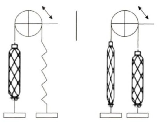
Figure 2.
Joint-to-pull mode.
The first way is achieved by using a pneumatic artificial muscle and a spring composed of a pulling mechanism. The second uses the antagonistic arrangement of a pair of antagonistic connections of the pulling pneumatic muscle. In comparison, the price of the first pneumatic muscle-spring combination is better than the second; the disadvantage is that this mechanism constitutes the antagonistic joint, and to achieve the same expected angle, the first requires a more considerable pneumatic muscle output tension than the second, which often reduces the service life of the pneumatic muscle. Moreover, in the control of the spring compared to the controllability of the pneumatic artificial muscle, jitter and other problems often arise with use. Furthermore, the long-time use of the spring can easily produce fatigue, resulting in control accuracy as well as elasticity decline, but it is suitable for the study of pneumatic artificial muscle’s own physical characteristics of the law. Therefore we use the structure of the PAM-PAM series pull-pair for dynamic characteristics simulation, control simulation, and control experiments. As the dynamic characteristics experiment is used to discuss and verify the physical properties of pneumatic artificial muscles, the use of PAM + spring also satisfies the requirements of studying the laws of PAM’s physical properties. From an economic viewpoint, the experiments on the dynamic characteristics of PAM in the thesis are conducted according to the PAM-spring structure.
The simulation model is established in the Matlab Simulink software according to Equations (1) and (2), (8)–(10), Figure 3 shows the pneumatic artificial muscle-driven joint model, and the parameters used in the simulation are shown in Table 1. Gas source temperature is given in degrees Kelvin, pneumatic muscle initial length and single fiber length in meters, valve port circulation effective cross-sectional area in square meters, upstream inflation pressure in MPa, gas constant in N·m·kg−1·K−1, connecting rod length in meters, load mass in kg, joint radius in meters, and damping factor in N·s·m−1.
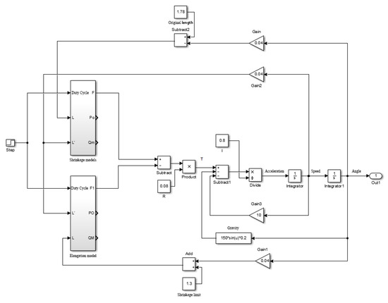
Figure 3.
Pneumatic artificial muscle-driven joint model.

Table 1.
Simulation parameter setting table.
Figure 4, Figure 5, Figure 6, Figure 7, Figure 8 and Figure 9 show the curves of each variable of the rotating joint model under the condition that the input signal is a step signal. The maximum joint rotation angle in Figure 4 and Figure 5 is about 68°, and the steady state time is 2 s. It can be seen from Figure 4 and Figure 5 that the single joint impact with pneumatic muscles is flexible and does not produce sudden changes in velocity acceleration.

Figure 4.
Angle and speed profile.
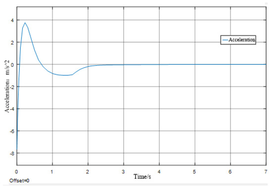
Figure 5.
Acceleration shift rate.
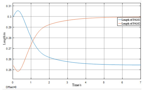
Figure 6.
PAM length curve.
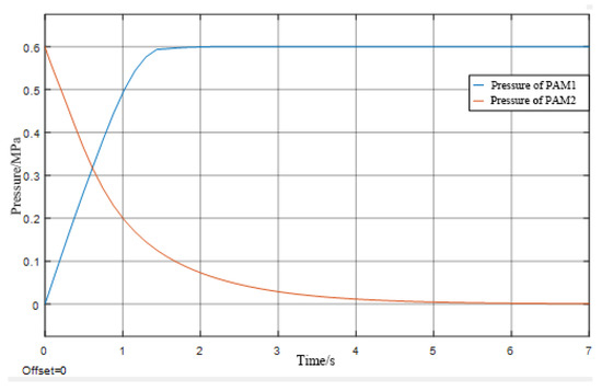
Figure 7.
PAM pressure curve.
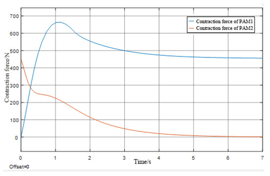
Figure 8.
PAM contraction force curve Figure.
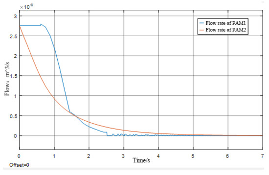
Figure 9.
PAM flow curve graph.
As can be seen in Figure 6 and Figure 7 below, the maximum contraction of the pneumatic muscles is 45 mm. Because of the antagonistic pullback relationship used in the model design, it can be seen from the images that the pressure and contraction relationships satisfy the complementary relationship, as shown in the following equation:
The pneumatic muscle can be analyzed in Figure 8 and Figure 9 to show that the maximum contraction force is 670 N when the joints are pulled against each other, which means that the single joint can be loaded with 67 kg. Since the simulation initially mimics PAM1 pulling PAM2 unilaterally in a pressure-holding state, the contraction side is inflated for some time and then stops. In contrast, the pressure-holding side is deflated slowly and regularly. The model, as shown in Figure 9, is consistent with reality.
The experimental results of the dynamic characteristics of the previous model are obtained by a series of operations. The relationship of the corresponding position change can be observed by simply changing the input pressure when the control variable method is studied. The shift corresponds to a good linear relationship, and the error is almost negligible, which can be seen from the comparison of Figure 4 and Figure 7; this pneumatic element is made of unique rubber and textile weave, so the movement is smooth, but there is rubber stretching viscosity so that the force output will inevitably have a certain amount of overshoot oscillation. The analytical model could be better in terms of length variation, especially in the case of low pressure and low load.
Therefore, the pneumatic circuit built by this pneumatic characteristic is generally used in lower limb rehabilitation robots; this does not respond to the healthcare situation and does not require a high response speed of the system. Accuracy and stability are the most critical requirements. Therefore, the use of closed-loop feedback adjustment to restrain the oscillation and overshoot is necessary [18].
3. PID Control Strategy Research Design
3.1. Introduction to PID Control Principle and Parameter Tuning
The PID control method is one of the most classic closed-loop control strategies, which is simple, reliable, and robust and is still widely used for process control of industrial and military-related equipment today. It is particularly suitable for deterministic control systems where an exact model can be built. It can also be used for non-accurate model control systems that rely on the empirical tuning of parameters. The PID control method is based on the output deviation, thus determining the size of the control link’s proportional P, integral I, and differential D link coefficients. In many closed-loop control systems, PID regulation is widely used in these controls; the PID control schematic is shown in Figure 10.
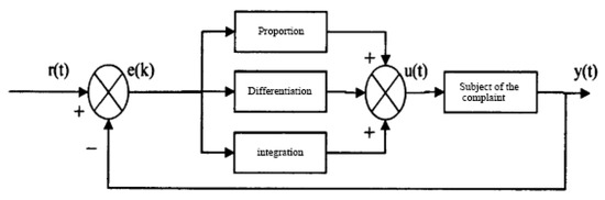
Figure 10.
PID control schematic.
The PID control equation is:
where r(t) is the given value of the system, y(t) is the actual output value of the system, e(t) is the deviation of the given value from the real output value, as the PID input value, and u(t) is the output value; there is a linear combination of deviation, e(t), constituted by a linear combination of the regulation of the error changes provided by the three parameters of the proportional parameter Kp, integral parameter Ki, and differential parameter Kd of the controlled object system. The central part of the PID control process is the adjustment of the three control parameters, also known as parameter tuning. The methods are generally theoretical calculation methods and engineering rectification methods. Among them, the pieced-together trial method is a standard engineering rectification method, relying on human experience regulation. Assume a certain parameter first, then adjust the parameter while observing the curve, and gradually determine the parameter according to the order of proportional, then integral and finally differential, until the control effect reaches the expectation. Taking the system modeling as an example, these three parameters of the system are listed as follows:
- (1)
- The principle of parameter adjustment when the error is significant. For the flow system, the control is faced with an amount of pneumatic muscle input flow volume through the high-speed switching valve. At this time, Kp regulation is like speeding up the forward step so that the law of the first time to reach the maximum overshoot time can be shorter; but this time also increases the generation of overshoot when the difference between the feedback value and the desired value is significant. To speed up the response of the control action, we take a correspondingly large Kp value and a small Kd value. Such a role can ensure that the I parameter gains effect and does not do useless work but causes the system to have a larger overshoot. Hence, the value of Ki is taken to be as small as possible; the closer to 0, the better. Of course, this is an ideal regulation, but generally, it cannot be so perfect. In addition, increasing the proportionality factor P in the case of static difference is conducive to reducing the static difference.
- (2)
- The principle of parameter adjustment when the error is medium. When the difference between the feedback value and the desired value is medium, the size of Kp often determines the speed of adjustment and the size of overshoot when the response time may be fast if Kd is significant. The amount of overshoot will still be substantial. The value of Kd should be chosen smaller at this time because Kd has a significant impact on the system. Moreover, Ki should also be given a proper value; Ki taking the appropriate value can often improve the phase response bias of the system’s sinusoidal response.
- (3)
- Adjustment principle when the error is small. When the difference between the feedback value and the desired value is slight, to ensure that the system has a high-quality regulation of the steady-state performance and that the oscillation will occur near its expected value, the value of Kp, Ki should be increased. Considering the system’s anti-interference ability, the position of the control produces irregular reciprocation in the predetermined position, and the principle of taking the differential parameter depends on the magnitude of the rate of change of the error. Generally, the value of the differential parameter should be chosen smaller when the error changes quickly and larger when the error changes slowly.
The PID control algorithm is implemented in the computer using sampling control, which requires the control process to be discretized, also known as digital PID. The discretized PID expression is:
where k is the sampling sequence number, uk is the computer output value at the kth is the sampling moment, ek is the deviation value of the input at the kth sampling moment, and ek−1 is the deviation value of the input at the (k − 1)th sampling moment. If the sampling interval is very short, Equation (12) yields very accurate results with discrete and continuous processes. Equation (12) gives each control quantity’s magnitude and is called positional PID.
In the position-based PID algorithm, each output is related to the past state, the calculation of ek accumulates, the analysis is large, and when the computer fails, the output uk will increase significantly. Incremental PID has none of these disadvantages. By putting the control variables in a discrete form, the discrete control curve will be infinitely close to the continuous control curve when the time interval of the sampling sequence number is small enough, and the incremental control variables can also avoid the generation of cumulative errors. The incremental PID control algorithm formula is:
Therefore, the incremental PID control algorithm is used in this paper.
3.2. MATLAB Modeling Response Analysis of PID Regulation
The open-loop control of joints is unsuitable for applications with high-performance requirements due to large oscillations in motion and poor repeatability of the position under step signal input. Thus, it is necessary to improve performance by using closed-loop control. This is shown in Figure 11.
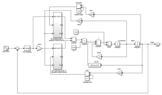
Figure 11.
Introduction of closed PID regulation modeling diagram.
The PID parameters of the system are now adjusted according to the critical proportionality method. Firstly, input Kp = 1, Ki and Kd = 0. It can be seen that there is a static error in the unit step response, which is because the contraction limit of the pneumatic muscle limits the joint angle that the two pairs of pull joints can eventually reach. The limit is 0.85 radians, which is about 48.7 degrees, as can be seen from the image data.
Due to the angle range limitation, the unit step input value should be 0.85, as shown in Figure 12, for the uncorrected step response. Figure 13 shows the schematic diagram of the unit step input of 28 degrees, and Figure 14 shows the square wave input of 28 degrees.
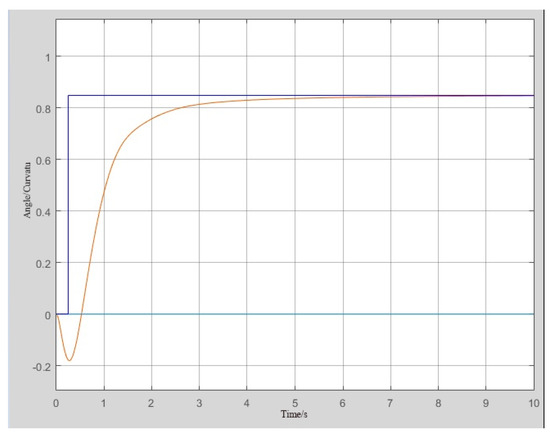
Figure 12.
48 degree step response curve of lower limb joints.
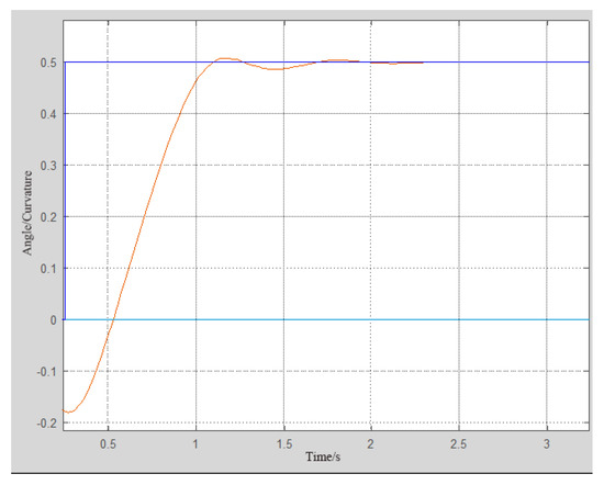
Figure 13.
28 degree step response curve of lower limb joints.
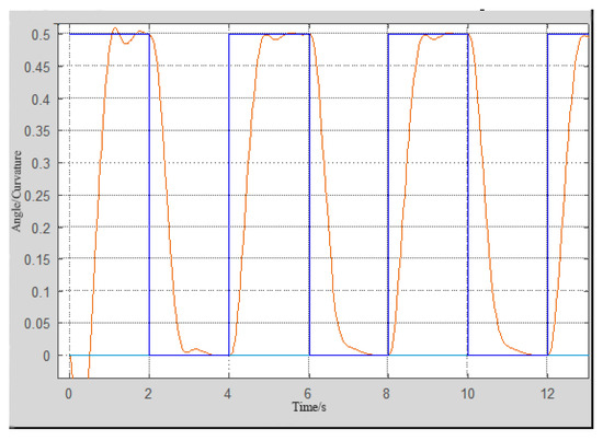
Figure 14.
Square wave signal response graph.
The analysis shown above shows that in the step response, as the preset desired angle decreases, the oscillation generated by the same PID parameters will increase the more minor the desired angle in regulation.
The transient response performance index can be derived from Figure 13.
The rise time can be measured as ts = 0.525 s − 0.310 s = 0.215 s; the peak time is tp = 0.64 s. The error curve of the overshoot oscillation at 28 degrees is shown below; when the input is 28 degrees, the step response to reach stability will appear in a certain amount of overshoot; Figure 13 shows an overshoot oscillation size of 0.02 radians, which translates into an angle of (−1.5, +1.5). The error is calculated from Equation (14):
where σ is the steady-state error. Moreover, as shown in Figure 14, the analysis of the square wave response can be seen after the PID regulation to a certain hysteresis of the system, which is related to the characteristics of the pneumatic muscles. In addition to the slow response speed, the stability and steady-state error are well controlled, so the error is permissible under the condition that the lower limb rehabilitator does not require high rapidity.
In summary, it can be seen that in this step response, the overshoot oscillations in the general system have met the steady-state error of 2–5% and, for the first time, reached 63% of the target of regulation as the time constant value, that is, the time constant T = 0.5 s, and the system in two time constants to achieve output stability. This proves that the system transient response steps are fast and stable, in line with our expectations and requirements.
4. Experimental Design of Pneumatic Artificial Muscle Control
4.1. The Principle and Construction of the Laboratory Table
Pneumatic artificial muscle mainly consists of a rubber tube. The fiber is a woven net wrapped around the tube with connectors at both ends, which can realize one-way linear movement and recovery movement by inflation/deflation. When inflated, the compressed gas enters the pneumatic artificial muscle cavity, the pressure inside the cavity is enhanced, the rubber tube of the pneumatic artificial muscle expands radially and drives the woven bag angle change, and the linear length direction of the pneumatic artificial muscle generates contraction force and drives the external load movement. When the compressed gas in the cavity is released, the radial and axial directions of the pneumatic artificial muscle are gradually restored to the original shape.
The general schematic diagram of this pneumatic artificial muscle control experiment bench is shown in Figure 15. The three experimental parameters to be measured are the external force part, the pressure of the pneumatic artificial muscle, and the length of the pneumatic artificial muscle. Among them, the external force part can be connected using another pneumatic artificial muscle to conduct the pull-off experiment; the external force part can also be connected to an external load. The external load is applied in two ways: one is obtained through the solenoid valve to control the cylinder expansion, and the other is obtained by adding a mass block at the end of the external force part; changing the number of mass blocks can be achieved by changing the size of the external force, which the tension sensor can measure. A pressure sensor reads the magnitude of the internal pressure of the pneumatic muscle. The original length of the pneumatic muscle is 300 mm, and the change in length can be calculated by measuring the angle of rotation of the timing pulley with an absolute angle encoder. The lower computer, STM32, collects the rotation angle value through the encoder. Then, after ordering, the STM32 sends the collected data to the upper computer, built by the LabVIEW software.
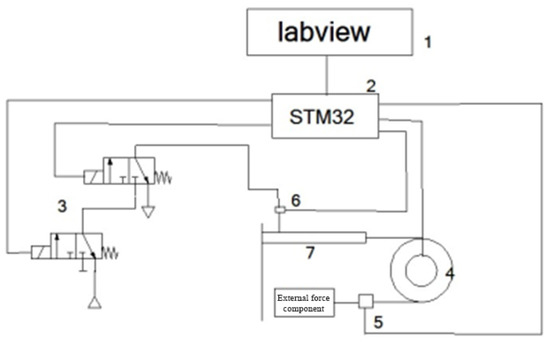
Figure 15.
General schematic diagram of the lab bench: 1—Labview upper computer; 2—STM32 lower computer; 3—two-position three-way solenoid valve; 4—angle encoder; 5—tension sensor; 6—compression sensor; 7—pneumatic manual muscle.
The structure of the pneumatic artificial muscle experimental stand and the names of the parts are shown in Figure 16.
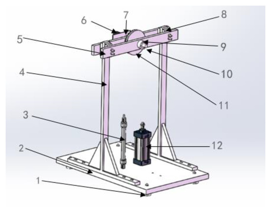
Figure 16.
Three-dimensional model of the experimental stand:1—Foot squat; 2—Base plate; 3—300 mm pneumatic muscle; 4—Left and right brackets; 5—Middle beam; 6—Angle encoder; 7—Angle encoder bracket; 8—Beam spacer; 9—Flange bearing; 10—Shaft; 11—Timing belt pulley; 12—Cylinder.
The main dimensions of the experimental stand are described as follows: the bottom plate is made of a 500 × 800 × 30 mm steel plate, on which the M10 bolt holes are drilled; the left and right brackets, foot squat, pneumatic manual muscle, and cylinder need to be drilled. The left and right brackets are made of 800 × 20 × 40 mm hollow square steel and 600 × 20 × 40 mm open square steel welded together, fixed on both sides with 200 mm height steel fascia plates, and the M10 bolt holes required for assembly are drilled on its top and bottom, the height of the whole bracket is 820 mm, and the length of the contact side with the base plate is 600 mm. The crossbeam is made of a 600 × 60 × 20 mm steel plate with M10 bolt holes drilled at both ends for attachment to the crossbeam and crossbeam spacer; a 30 mm diameter through-hole is positioned in the middle for shaft passage and a threaded hole for flange bearing attachment. The beam spacer is 80 × 40 × 20 mm hollow square steel with M10 holes for fixing. The pulley is a timing belt pulley, which is mounted coaxially with the shaft on the middle cross beam. The port of the synchronous belt is connected to a section of the pneumatic artificial muscle with the interface, and the experiment is carried out by the reciprocal contraction movement of the pneumatic artificial muscle; the pulley is then rotated by the synchronous belt on the wheel. The reason for choosing the timing pulley is that the static pulley is easy to slip and will cause inaccurate angle measurement, which will affect the measured amount of pneumatic artificial muscle length change, thus making the experimental results incorrect. The timing pulley used for the experiment was custom-made on the Mismi with a radius of 75.74 mm.
4.2. Experimental Design of Pneumatic Artificial Muscle Dynamic Characteristics
The dynamic characteristics of the pneumatic artificial muscle experiments test are that the pneumatic artificial muscle, in the case of constant external load, suddenly opens or closes the solenoid valve so that the pneumatic artificial muscle inflation or deflation, used to measure the change curve of its internal pressure in the process of inflation becomes shorter; if deflation becomes longer, the length of the curve of the pneumatic artificial muscle changes. Its schematic diagram is shown in Figure 17, and Figure 18 is its physical diagram.
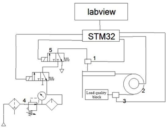
Figure 17.
Schematic diagram of dynamic characteristics experiment: 1—Pressure sensor; 2—Angular encoder; 3—Tension sensor; 4—Pneumatic triplex; 5—Two-position three-way solenoid valve.
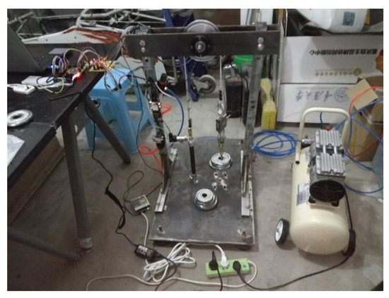
Figure 18.
Physical diagram of dynamic characteristics experiment.
The experimental process is as follows: add a mass block of 1.5 kg at one end of the timing pulley, adjust the pressure inside the pneumatic artificial muscle to 0.3 MPa through the triplet, then click the inflation in the upper computer program, the solenoid valve will open, and the pneumatic muscle will start to inflate, after the pneumatic artificial muscle is stabilized, click the deflation button in the upper computer program, the pneumatic muscle will start to deflate under the control of the solenoid valve. The lower computer collects the experiment’s data according to a specific time interval, and it is saved after processing. The data measured in the investigation is the change in the length of the pneumatic muscle and the evolution of its internal pressure after the start of inflation or deflation. After that, adjust the pressure-reducing valve in the triplet to control the pressure inside the pneumatic artificial muscle to 0.5 MPa, and carry out the experiment according to the same experimental steps, totaling four groups of experiments. After completing the experiment using a 1.5 kg block, replace the mass block mass with 4 kg and repeat the above experimental steps. The experiment included a total of eight groups.
4.3. Experimental Design of Pneumatic Artificial Muscle Pair Pull
The physical construction now allows the drawing of a sketch of the system, as shown in Figure 19; the control of the joint angle only controls a single side of the pneumatic muscle. The control principle is to control the opening and closing of the electronically controlled high-speed switching valve through the combination of two two-position three-way high-speed switching valves to achieve the single pneumatic muscle pressure-holding, inflation, and deflation of the three processes.
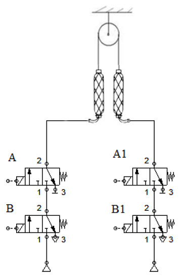
Figure 19.
Sketch of single-joint pull-apart system.
The system control process is briefly described as follows:
(1) System initialization; To simplify the experimental steps as much as possible, first, the two pneumatics were simultaneously manually inflated and adjusted to the same pressure; that is, the two pneumatic muscles are full of gas. After that, the fixed pulley will be adjusted to the middle state;
(2) The LabVIEW software experimental panel allows you to enter the desired angle value; programming will achieve the control of valves A and B, as shown. Control constitutes negative feedback of the angle, and the algorithm is achieved through PID regulation;
(3) The upper computer, through the LabVIEW software, allows you to achieve real-time monitoring of the angle adjustment process and record the generated data.
To design a program to control each action and achieve more intuition, the following figure shows the system action’s true value table; through a combination of A and B actions, you can achieve different action purposes. The value of “1” represents that the valve is powered in the left position of the two-way, three-way valve. The value of “0” means that the pneumatic solenoid’s fast switching valve is de-energized and is in the correct position of the two-way, three-way valve.
Therefore, to have a precise correspondence term in the PWM, duty cycle output needs to distinguish the action response of open and closed, i.e., the result of the action with or without correspondence on behalf of the input wave. The details are shown in Table 2 below.
Table 2.
System action truth table.
As summarized in Table 2 above, the control of inflation means that the A and B valves are electrically energized simultaneously. In contrast, the control of deflation means that only the A input is electrically energized because the high-speed switching valve can be automatically reset. The overall control of the feedback is to use the complementary pull of the two pneumatic muscles to achieve control of the predetermined angle. In addition, the available pneumatic solenoid high-speed switching valve switching frequency is in the range of 100~250 Hz; this frequency is ten times higher than the maximum frequency that the pneumatic muscle can respond to, so it meets the control requirements; to achieve reasonable control of the pneumatic muscle, the experimental design uses 150 Hz as this switching frequency.
The schematic diagram of the pull-apart experiment is shown in Figure 20, while Figure 21 shows the physical diagram of the actual built pull-apart experimental platform. The central units include the air and valve control system and the upper computer. The central axis of joint rotation is placed with an encoder with a resolution of 0.3515625° and a sampling frequency of 10.42 khz to achieve real-time feedback of the collective angle information. Real-time tasks such as pneumatic tendon control commands, air pressure adjustment of the valve control system, and data acquisition of sensors are unified by the host computer for task management, resource allocation and scheduling. During the test, the control command of the desired trajectory is issued by the host computer, which is sent to the STM32F103ZET6 control board through the USB-TTL serial port and then servo-controlled by the valve control system for the pneumatic manual muscle. At the same time, the joint angle is returned to the upper mechanism in real-time at the same frequency to form a closed system loop.

Figure 20.
Antagonistic joint dynamics and control test schematic: 1—labview upper computer; 2—STM32 lower computer; 3—high-speed switching solenoid valve; 4—absolute angle encoder; 5—inertial load; 6—pneumatic muscle.
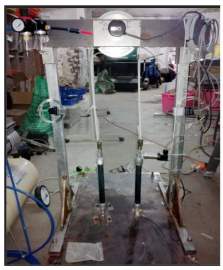
Figure 21.
Physical diagram of the pair-pulling experiment.
5. Experimental Results and Analysis
5.1. Analysis of Dynamic Characteristics Experimental Results
The experimental plots of dynamic characteristics are shown in Figure 22, Figure 23, Figure 24, Figure 25, Figure 26, Figure 27, Figure 28 and Figure 29, where Figure 22, Figure 23, Figure 24 and Figure 25 show the variation of pneumatic artificial muscle length with time, and Figure 26, Figure 27, Figure 28 and Figure 29 show the variation of internal pressure of pneumatic artificial muscle with time. The plot lines with black dots in the figures are the experimental data curves, and the smooth curves are the simulation curves.

Figure 22.
Pneumatic artificial muscle length change graph under a load of 1.5 kg and a pressure of 0.3 MPa.
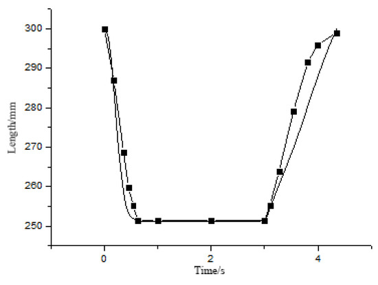
Figure 23.
Pneumatic artificial muscle length change graph under a load of 1.5 kg and a pressure of 0.5 MPa.
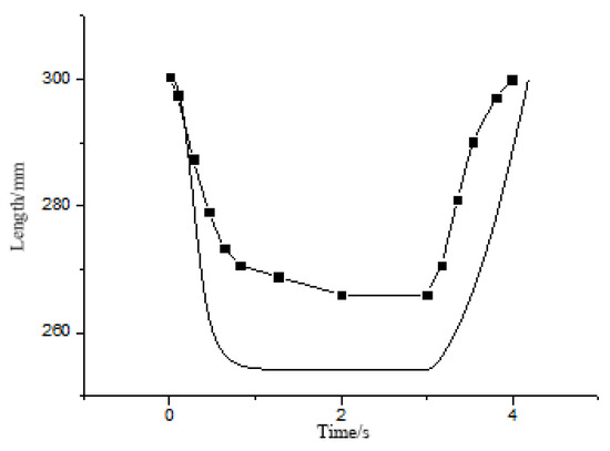
Figure 24.
Pneumatic artificial muscle length change graph under a load of 4 kg and a pressure of 0.3 MPa.
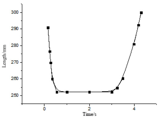
Figure 25.
Pneumatic artificial muscle length change graph under a load of 4 kg and a pressure of 0.5 MPa.

Figure 26.
Internal pressure change of pneumatic artificial muscle under a load of 1.5 kg and a pressure of 0.3 MPa.
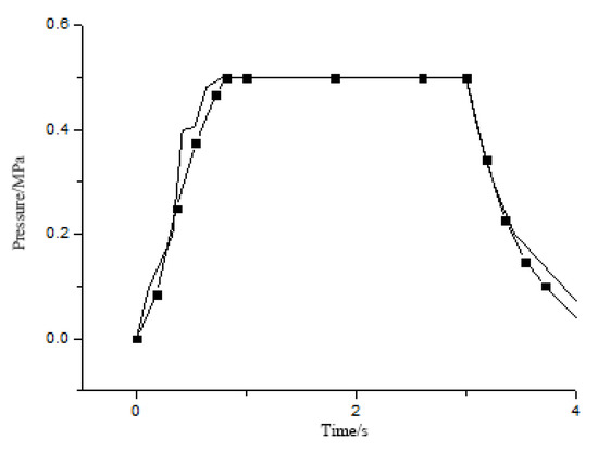
Figure 27.
Internal pressure change of pneumatic artificial muscle under a load of 1.5 kg and a pressure of 0.5 MPa.
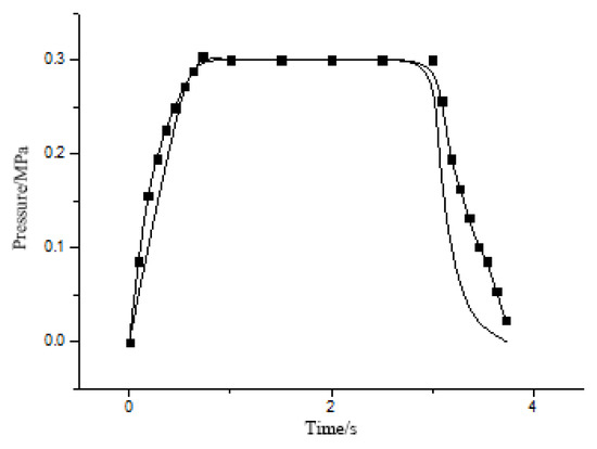
Figure 28.
Internal pressure change of pneumatic artificial muscle under a load of 4 kg and a pressure of 0.3 MPa.
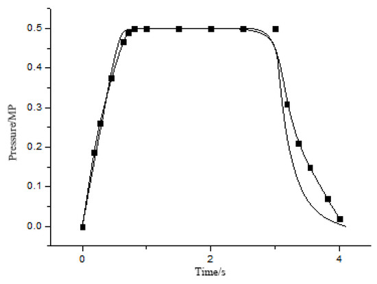
Figure 29.
Internal pressure change of pneumatic artificial muscle under a load of 4 kg and a pressure of 0.5 MPa.
From Figure 22, Figure 23, Figure 24 and Figure 25, it can be seen that at 0.3 MPa, there is a big difference between the theoretical model and the actual model, and at 0.5 MPa, the difference between the actual model and the theoretical model is very small. With an increase in pressure inside the pneumatic muscle, the difference between the actual and the theoretical is smaller and smaller. The main reason may be that the elasticity of rubber and the influence of friction between the woven mesh and rubber should be considered when establishing the static model of the pneumatic muscle. Because friction and elasticity will hinder the movement of the pneumatic muscle, the actual change length is smaller than the theoretical change length. In addition, the lower the air pressure, the larger the gap, which indicates that the lower the air pressure, the greater the relative influence of elasticity and friction may also be.
From Figure 26, Figure 27, Figure 28 and Figure 29 above, it is easy to see that the actual internal pneumatic muscle pressure change relationship with time is in good agreement with the theoretical model. When the load is 4 kg, the actual curve of pneumatic muscle is under 0.3 MPa, and 0.5 MPa conditions have a slight separation from the theoretical curve, which is due to the friction between the woven mesh and rubber consuming energy, which will slow down the speed of the pneumatic muscle movement, thus slowing down the decline of the internal pressure of the pneumatic muscle. Moreover, the theoretical model does not consider the two factors of elasticity and friction, so there will be some deviation.
5.2. Analysis of Experimental Results of Pneumatic Artificial Muscle Butt Pull Step
Figure 30 shows the pneumatic artificial muscle pulling experiment; the pressure of the air source is set to 0.5 MPa, and the range of movement angle of each joint is set to the average for a human lower limb, taken from the literature [19]. Combined with the experimental conditions and effects, we take an intermediate value to meet each joint, so the experimental results of the given step signal input is 45°:
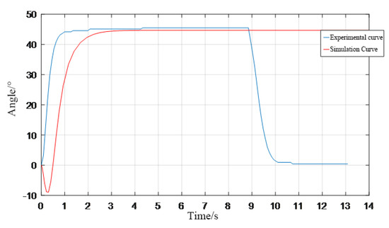
Figure 30.
Experimental response graph of step signal 45°.
Figure 30 shows the simulation for 45° and the experimental 45° control step response graph; as can be seen in the graph, there is consistency between the two transients. Still, the simulation curve is relatively more lagging, about 0.5 s; considering that the damping of the pneumatic artificial muscle may be too large, the signal curve response lag has some impact.
Then the transient response performance index can be derived from Figure 29: the rise time of the experimental curve is ts = 0.6 s and − 0.1 s = 0.5 s; its peak time is tp = 2 s; the experimental curve will not overshoot oscillation when the input 45° step response reaches stability, indicating that the system output is stable. Taking T(60%) = 0.4 s as the time constant of reference, then 2 T = 42.75°/45° × 100% = 95%, meaning that the system can reach 95% of the desired value of the rise in two cycles, which also further confirms that the system response speed is sufficient.
6. Discussion
The experimental results were obtained according to the model’s design and experiments in the previous sections. After that, the data results obtained from the experiments were processed, and the experimental results were compared and analyzed with the theoretical modeling results. It was found that the theoretical dynamic model of the pneumatic muscle at 0.5 MPa in the dynamic characteristics experiment was more consistent with the actual experimental situation. Still, because of the complexity of the gas flow inside the pneumatic artificial muscle and the mutuality of the fundamental forces on the external motion, the error was relatively more significant when the pressure was less than 0.5 MPa; for 0.3 MPa, the error was somewhat larger. Moreover, the proposed PID algorithm can meet the requirements of stability as well as accuracy for the daily work of this pneumatic artificial muscle; it is only lacking in rapidity.
7. Conclusions
With an increasingly urgent demand for lower limb rehabilitation robots in today’s society, pneumatic artificial muscle, based on a large amount of research literature, is popular for its core drive element. We compared previous modeling and control strategy analysis of pneumatic muscles through the study of fluid mechanics and thermodynamics to establish a pneumatic muscle, and the modeling and control strategy analysis of pneumatic muscles are compared. A more realistic mechanics model of the pneumatic muscle is established through fluid dynamics and thermodynamics analysis. Then we analyzed the principle of PID control strategy and the method of PID parameter adjustment and built the dynamic characteristics via an experimental bench; we also carried out the dynamic characteristics and adaptive control experiments of the pneumatic artificial muscle. The validity of the model and the effectiveness of PID regulation on the joint control system of pneumatic artificial muscles were verified through various experiments. Although there is a lack of rapidity, the main requirement for pneumatic artificial muscle in lower limb rehabilitation robots is stability and accuracy, so its control is in line with the design requirements. However, the static model of pneumatic artificial muscle has some shortcomings, as it needs to sufficiently take into account the influence of the elasticity of the rubber tube on itself and the result of the friction between the woven mesh and the rubber. Moreover, from the experimental control portability and the limitations of STM32, only the PID control algorithm was selected as the control strategy. Still, a priori verification was made for future improvements to the control strategy. The design and improvement of control strategies for pneumatic artificial muscles in the future will be a significant research area for lower limb rehabilitation robots.
Author Contributions
G.H. provided the idea and project direction, provided the lab and project funding, and provided writing comments on the paper. J.M. refined the theoretical derivation and model building, completed the experiments and wrote the paper. J.Y. provided help in researching the literature and theoretical derivation. All authors have read and agreed to the published version of the manuscript.
Funding
Supported by the National Key R & D plan of the Ministry of Science and Technology (2019yfb1703600) and the Key project of National Natural Science Foundation of China (62033001).
Institutional Review Board Statement
Not applicable.
Informed Consent Statement
Not applicable.
Data Availability Statement
Data sharing is not applicable. No new data were created or analyzed in this study. Data sharing is not applicable to this article.
Conflicts of Interest
The authors declare no conflict of interest.
References
- Kong, K.; Bae, J.; Tomizuka, M. A Compact Rotary Series Elastic Actuator for Human Assistive Systems. IEEE/ASME Trans. Mechatron. 2012, 17, 288–297. [Google Scholar] [CrossRef]
- Yanbin, L.; Xiangyuan, P.; Yanbin, Z.; Bingjing, G.; Jianhai, H. Research on Active Training Compliance Control of Ankle Rehabilitation Robo. J. Syst. Simul. 2020, 32, 54–60, (In Chinese with English Abstract). [Google Scholar] [CrossRef]
- Binrui, W.; Weiyi, Z.; Hong, X. Static Actuating Characteristics of Intelligent Pneumatic Muscle. Trans. Chin. Soc. Agric. Mach. 2009, 40, 208–212+193, (In Chinese with English Abstract). [Google Scholar]
- Li, B.; Liu, J.; Yang, G. Modeling and Simulation of Pneumatic Muscle System. J. Mech. Eng. 2003, 39, 23–28. [Google Scholar] [CrossRef]
- Zang, K.; Gu, L.; Tao, G. Study and Prospect of Pneumatic Artificial Muscles. Mach. Tools Hydraulics 2004, 4, 4–7+111, (In Chinese with English Abstract). [Google Scholar] [CrossRef]
- Chou, C.-P.; Hannaford, B. Static and dynamic characteristics of McKibben pneumatic artificial muscles. In Proceedings of the IEEE International Conference on Robotics & Automation, San Diego, CA, USA, 8–13 May 1994; IEEE: Piscataway, NJ, USA, 1994. [Google Scholar] [CrossRef]
- Tondu, B.; Lopez, P. Modeling and control of McKibben artificial muscle robot actuators. Control. Syst. Mag. 2000, 20, 15–38. [Google Scholar] [CrossRef]
- Reynolds, D.B.; Repperger, D.W.; Phillips, C.A.; Bandry, G. Modeling the dynamic characteristics of pneumatic muscle. Ann. Biomed. Eng. 2003, 31, 310–317. [Google Scholar] [CrossRef] [PubMed]
- Tondu, B. Static Modeling of Pneumatic Artificial Muscle Actuator. In Proceedings of the 5th IEEE International Conference on Soft Robotics (RoboSoft), Edinburgh, UK, 4–8 April 2022; Volume 2022, pp. 364–369. [Google Scholar] [CrossRef]
- Wang, Y.; Jin, Q.; Zhang, R. Improved fuzzy PID controller design using predictive functional control structure. ISA Trans. 2017, 71, 354–363. [Google Scholar] [CrossRef] [PubMed]
- Cheng, Z.; Lei, G. Towards a theoretical foundation of PID control for uncertain nonlinear systems. Automatica 2022, 142, 110360. [Google Scholar] [CrossRef]
- Wang, J.; Liu, Y.; Jin, Y.; Zhang, Y. Control of Hydraulic Power System by Mixed Neural Network PID in Unmanned Walking Platform. J. Beijing Inst. Technol. 2020, 29, 273–282. [Google Scholar] [CrossRef]
- Repperger, D.; Johnson, K.; Phillips, C. A VSC position tracking system involving a large scale pneumatic muscle actuator. In Proceedings of the IEEE Conference on Decision and Control, Tampa, FL, USA, 18 December 1998; Volume 4, pp. 4302–4307. [Google Scholar] [CrossRef]
- Hesselroth, T.; Sarkar, K.; van der Smagt, P.; Schulten, K. Neural Network Control of a Pneumatic Robot Arm. IEEE Trans. Syst. Man Cybern. 1994, 24, 28–37. [Google Scholar] [CrossRef]
- Lilly, J.H. Adaptive tracking for pneumatic muscle actuators in bicep and tricep configurations. IEEE Trans. Neural Syst. Rehabil. Eng. 2003, 11, 333–338. [Google Scholar] [CrossRef] [PubMed]
- Tondu, B.; Ippolito, S.; Guiochet, J.; Daidie, A. A Seven-degrees-of-freedom Robot-arm Driven by Pneumatic Artificial Muscles for Humanoid Robots. Int. J. Robot. Res. 2005, 24, 257–274. [Google Scholar] [CrossRef]
- Zhu, X.; Tao, G.; Yao, B.; Cao, J. Adaptive robust posture control of a parallel manipulator driven by pneumatic muscles. Automatica 2008, 44, 2248–2257. [Google Scholar] [CrossRef]
- Fortuna, L.; Frasca, M.; Buscarino, A. Optimal and Robust Control: Advanced Topics with MATLAB; CRC Press: Boca Raton, FL, USA, 2012; pp. 1–2311. [Google Scholar] [CrossRef]
- Xiang, W. Research on Design and Joint Control of Pneumatic Tendon-Driven Lower Limb Rehabilitation Robot. Master’s Thesis, College of Mechanical and Vehicle Engineering, Chongqing University, Chongqing, China, 2020; pp. 18–19. [Google Scholar] [CrossRef]


Disclaimer/Publisher’s Note: The statements, opinions and data contained in all publications are solely those of the individual author(s) and contributor(s) and not of MDPI and/or the editor(s). MDPI and/or the editor(s) disclaim responsibility for any injury to people or property resulting from any ideas, methods, instructions or products referred to in the content. |
© 2023 by the authors. Licensee MDPI, Basel, Switzerland. This article is an open access article distributed under the terms and conditions of the Creative Commons Attribution (CC BY) license (https://creativecommons.org/licenses/by/4.0/).