Multiple Elimination Based on Mode Decomposition in the Elastic Half Norm Constrained Radon Domain

Abstract

Multiple reflection is a common interference wave in offshore petroleum and gas exploration, and the Radon-based filtering method is a frequently used approach for multiple removal. However, the filtering parameter setting is crucial in multiple suppression and relies heavily on the experience of processors. To reduce the dependence on human intervention, we introduce the geometric mode decomposition (GMD) and develop a novel processing flow that can automatically separate primaries and multiples, and then accomplish the suppression of multiples. GMD leverages the principle of the Wiener filtering to iteratively decompose the data into modes with varying curvature and intercept. By exploiting the differences in curvature, GMD can separate primary modes and multiple modes. Then, we propose a novel sparse Radon transform (RT) constrained with the elastic half (EH) norm. The EH norm contains a $l_{1/2}$ norm and a scaled $l_2$ norm, which is added to overcome the numerical oscillation problem of the $l_{1/2}$ norm. With the help of the EH norm, the estimated Radon model can reach a remarkable level of sparsity. To solve the optimization problem of the proposed sparse RT, an efficient alternating multiplier iteration algorithm is employed. Leveraging the high sparsity of the Radon model obtained from the proposed transform, we improve the GMD-based multiple removal framework. The high-sparsity Radon model obtained from the proposed Radon transform can not only simplify the separation of primary and multiple modes but also accelerate the convergence of GMD, thus improving the processing efficiency of the GMD method. The performance of the proposed GMD-based framework in multiple elimination is validated through synthetic and field data tests.

1. Introduction

The ocean holds substantial reserves of petroleum and gas resources. Seismic exploration serves as the initial step in offshore petroleum and gas exploration and development, and the quality of seismic data directly impacts the subsequent petroleum and gas hydrate exploration [1,2,3,4]. When conducting offshore seismic acquisition, due to the strong wave impedance difference between seawater and air, seismic acquisition data contain multiples in addition to primaries. Multiples can cover the effective signals and hinder the imaging and identification of subsurface geological structures. To enhance data quality and achieve a more precise identification of subsurface targets, it becomes imperative to suppress multiples. One commonly employed technique for multiple suppression is the Radon transform-based filtering method. The Radon transform (RT) is a classical transformation [5] and has been extensively used in seismic exploration for various purposes such as multiple elimination, denoising, deblending, and interpolation [6,7,8,9,10,11]. Primaries and multiples exhibit different move-out characteristics in a Common Midpoint (CMP) gather. After applying the normal move-out (NMO) correction, primaries are corrected from hyperbolic to linear, whereas multiples are corrected from hyperbolic to parabolic, exhibiting a residual move-out. Using the parabolic RT, multiples and primaries are located in variant regions in the Radon domain due to their variation in curvature. Subsequently, a filter is utilized to mute the multiple coefficients, and the final demultiple result is obtained by performing the inverse RT to the filtered Radon model [12,13]. This is the fundamental theory of why and how the Radon filter method can be used for multiple suppression. However, when using the filter method for multiple elimination, it is crucial to set appropriate filtering parameters. These parameters are heavily dependent on the experience of geophysicists. If the filtering parameters are set improperly, the filtered result will either contain multiple residuals or hurt primaries [6]. Complicating matters further, the optimal filtering parameters for one area may not be suitable for another due to the inherent differences in seismic data. It requires processors to pay sufficient attention to ensure whether the processing parameters are appropriate for the input data. Therefore, developing a demultiple method that does not rely on manual parameters setting is currently an urgent need in the petroleum industry.

Empirical mode decomposition (EMD) [14,15,16,17] and variational mode decomposition (VMD) [18,19,20] are two signal-processing methods that can automatically decompose signals into several intrinsic mode functions based on a predefined number of modes. Geometric mode decomposition (GMD) [21], inspired by VMD, is an innovative approach in signal analysis that enables the decomposition of a 2D seismic data into several modes with various geometric characteristics. These geometric features include principal slopes and curvatures. GMD designs a new objective function and adaptively obtains geometric parameters by minimizing the variational energy along different directions. Using the alternating direction method of multipliers (ADMM) algorithm [22,23], the optimization problem of GMD can be solved, and the mode decomposition can be achieved. GMD contains two components: GMD-F, which performs decomposition in the frequency domain, and GMD-R, which performs decomposition in the Radon domain. The GMD-F algorithm can be utilized to separate diffractions based on the kinematic and dynamic disparities between reflections and diffractions in the f-k domain [24]. GMD-R leverages the principle of the Wiener filter to iteratively decompose the input data into modes with varying curvatures and intercept times. After NMO correction, there are curvature differences between multiples and primaries. As a result, the separation of primary and multiple modes can be achieved using GMD-R. Based on GMD-R, we have developed a framework for automatically separating primary and multiple modes in the Radon domain. Compared to the Radon filter method, the developed GMD-based multiple suppression method significantly reduces the need for human intervention, as GMD-R automatically performs computational decomposition based on the predefined number of modes. However, the result of GMD-R is dependent on the resolution and sparsity of the Radon model, which is affected by the limited sampling and finite aperture in offset [25].

To address the challenges associated with achieving a high-resolution Radon model, RT is regarded as an inversion problem, and various inversion methods are employed to solve this problem [6]. In 1995, Sacchi et al. [26] presented a new approach to achieve sparse Radon transform, implementing it in the frequency domain (FSRT) through a Bayesian framework. While this algorithm proved to be highly efficient, its limitation lies in the fact that RT in the frequency domain assigns equal weight to all events, constraining its ability to enhance temporal resolution. In response to this constraint, the time domain sparse RT (TSRT) was introduced [27], offering a higher level of sparsity in the time domain and thereby achieving enhanced resolution. However, it is worth noting that TSRT comes with a substantial computational cost [28]. Combining the advantages of TSRT and FSRT, a novel RT was developed by Trad et al. [6]. The approach performs RT and its inverse in the frequency domain, formulates a new equation with the $l_1$ norm constraint, and solves it iteratively using the re-weighted least-squares algorithm. However, the large dimension of the inverse matrix in the time domain leads to a high computational cost. To overcome this disadvantage, an iterative 2D model shrinkage algorithm was introduced by Lu to accelerate the RT [29]. Gholami et al. employed an iterative algorithm that combines the Radon transform with a $l_1$ norm regularization term for denoising and spares the representation of seismic data [30]. A new sparse RT was proposed by Wang et al. to attenuate the outlier effects in the Radon domain [31]. Kazemi and Sacchi developed a new RT along the offset direction and modified the basic Radon function to alleviate the ill-posed problem [32]. Furthermore, Geng et al. developed a novel sparse RT with the $l_{1-2}$ norm constraint (SRTL₁₋₂) and extended the method to three dimensions for multiple attenuation [33,34]. The $l_p$ norm is added to promote sparsity of RT [35,36]. However, the method is computationally complex and requires a large number of iterative operations.

To enhance the sparsity of the Radon model while concurrently reducing computational complexity, this paper introduces the elastic half (EH) norm [37,38] as a constraint on the RT and proposes a sparse Radon transform. The EH norm contains a $l_{1/2}$ norm and a scaled $l_2$ norm, which is added to overcome the numerical oscillation problem of the $l_{1/2}$ norm. To solve the optimization problem of the developed sparse RT, an efficient alternating multiplier iteration algorithm is employed. Then, we improve the GMD-based demultiple framework by applying GMD-R to the sparse Radon model of the proposed RT. The high-sparsity Radon model can not only simplify the separation of primary and multiple modes but also improves the computational efficiency of GMD-R. In addition, we conduct an analysis of the impact of the number of mode decompositions and provide recommendations for selecting an appropriate number. Finally, synthetic and field dataset tests are given to verify the favorable performance of the proposed GMD-based approach in multiple elimination.

2. Methods

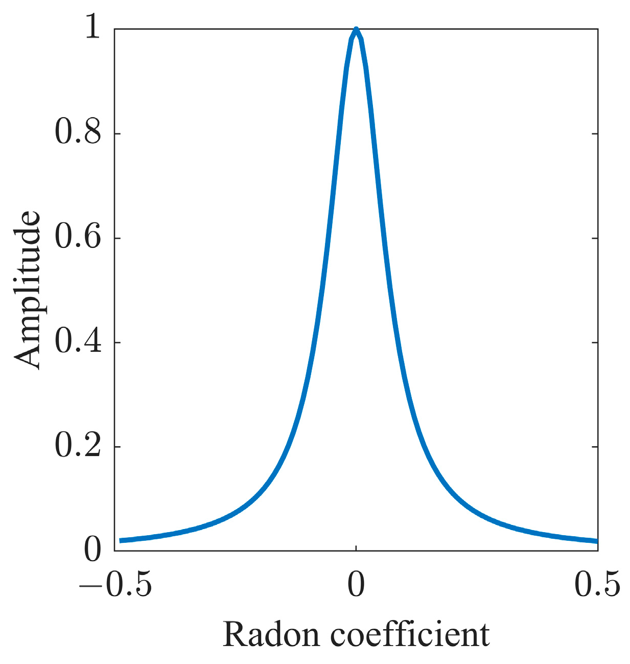
2.1. Sparse Radon Transform with the Elastic Half-Norm Constraint

In seismic exploration, the 2D forward RT [6,39] and its inverse are given by

$$\begin{gathered} m\left(\tau ,q\right)={\displaystyle \sum _{x=x_{\min }}^{x=x_{\max }}d\left(t=\tau +q{x}^{Ns},x\right),} \\ d\left(t,x\right)\approx {\displaystyle \sum _{q=q_{\min }}^{q=q_{\max }}m\left(\tau =t-q{x}^{Ns},q\right)}, \end{gathered}$$

(1)

where $d\left(t,x\right)$ denotes the input seismic data and $m\left(\tau ,q\right)$ represents the estimated Radon model. The variables $\tau , q, Ns$ in Equation (1) represent the intercept time, slowness, and integration stack path [39,40]. We can perform the transform in the frequency domain, and the above equation can be represented by [6]

$$\begin{gathered} M\left(\omega ,q\right)={\displaystyle \sum _{x=x_{\min }}^{x=x_{\max }}D\left(\omega ,x\right)}{\mathrm{e}}^{i\omega q{x}^{Ns}}, \\ D\left(\omega ,x\right)={\displaystyle \sum _{q=q_{\min }}^{q=q_{\max }}M\left(\omega ,q\right)}{e}^{-i\omega q{x}^{Ns}}, \end{gathered}$$

(2)

where $D\left(\omega ,x\right)$ and $M\left(\omega ,q\right)$ represents the frequency components of $d\left(t,x\right)$, and $m\left(\tau ,q\right)$, respectively. To simplify the derivation, Equation (2) can be represented by

$$\begin{gathered} M=L^{H}D, \\ D=LM, \end{gathered}$$

(3)

in which $L$ denotes the operator of the adjoint RT and $L^H$ is the conjugate transpose operator. The specific expression of $L$ is expressed as [31]

$$L=\left[\begin{array}{ccccc}{e}^{-i\omega q_1{x}_1^{Ns}}& e^{-i\omega q_2{x}_1^{Ns}}& \cdots & e^{-i\omega q_{nq-1}{x}_1^{Ns}}& e^{-i\omega q_{nq}{x}_1^{Ns}}\\ e^{-i\omega q_1{x}_2^{Ns}}& e^{-i\omega q_2{x}_2^{Ns}}& \cdots & e^{-i\omega q_{nq-1}{x}_2^{Ns}}& e^{-i\omega q_{nq}{x}_2^{Ns}}\\ ⋮& ⋮& \ddots & ⋮& ⋮\\ e^{-i\omega q_1{x}_{nx-1}^{Ns}}& e^{-i\omega q_2{x}_{nx-1}^{Ns}}& \cdots & e^{-i\omega q_{nq-1}{x}_{nx-1}^{Ns}}& e^{-i\omega q_{nq}{x}_{nx-1}^{Ns}}\\ e^{-i\omega q_1{x}_{nx}^{Ns}}& e^{-i\omega q_2{x}_{nx}^{Ns}}& \cdots & e^{-i\omega q_{nq-1}{x}_{nx}^{Ns}}& e^{-i\omega q_{nq}{x}_{nx}^{Ns}}\end{array}\right].$$

(4)

The number of rows and columns in the matrix $L$ is nx and nq, with nx being the trace number of input data and nq being the sampling number of slowness in the Radon domain, respectively. Using the 1D forward Fourier transform $f[·]$ and the inverse transform $f^{-1}[·]$, Equation (3) can be written as [41]

$$d=f^{-1}\left(Lf\left(m\right)\right).$$

(5)

However, the RT encounters challenges in cases when the input data have limited offsets and samplings [25]. These limitations lead to issues such as low resolution, aliasing, and overlapping events in Radon space. The low-resolution Radon model poses difficulties in accurately separating primaries from the input data. To address the problem of low resolution, the RT is always treated as a sparse inverse problem, and the sparse Radon model can be obtained by solving the equation as follows [6,33]

$$\underset{m}{\arg \min }{\Vert d-f^{-1}\left(Lf\left(m\right)\right)\Vert }_2^2+\lambda U\left(m\right),$$

(6)

where $U\left(m\right)$ denotes the constraint term, which plays a role in ensuring the solution is stable and unique. In general, $U\left(m\right)$ has different types, such as $l_0$, $l_{1/2}$ and $l_1$ norm. The $l_0$ norm provides the sparsest metric, but its solution is computationally challenging due to the nondeterministic polynomial time complexity. The $l_1$ norm is relatively easier to solve, but it does not yield a sparse enough solution [33]. In recent years, the $l_{1/2}$ norm regularization has received increasing attention and has been applied to solving inverse problems in various categories, as the $l_{1/2}$ norm has a stronger sparsity and robustness than the $l_1$ norm. However, the $l_{1/2}$ norm is nonconvex and may cause the solution unstable. To address the issue, Lan et al. [37] proposed an elastic half (EH) norm regularization to improve the $l_{1/2}$ norm constraint. Containing both Tikhonov and sparse regularization in the equation, the elastic half norm effectively mitigates numerical oscillation when dealing with ill-conditioned inverse problems. This leads to an optimal solution that exhibits improved sparsity and stability. Based on this, we propose a novel sparse Radon transform with the EH norm constraint and denote the method as EH-SRT. The method formulates the optimization problem as follows:

$$m*=\underset{m}{\arg \min }\frac{1}{2}{\Vert d-f^{-1}\left(Lf\left(m\right)\right)\Vert }_2^2+\lambda {\Vert m\Vert }_{1/2}^{1/2}+\sigma {\Vert m\Vert }_2^2,$$

(7)

where ${\Vert ·\Vert }_{1/2}^{1/2}$ represents the $l_{1/2}$ norm, $\lambda$ denotes the regularization parameter, and $\sigma$ is the scaling parameter. Comparing Equation (7) with the normal $l_{1/2}$ norm, one can find that there is an additional $\sigma {\Vert m\Vert }_2^2$ term, which is used to guarantee a stable and unique solution, because it solves the problem of numerical oscillations induced by the non-conductivity of the conventional $l_{1/2}$ norm at zero. If $\sigma =0$, the EH norm regularization will convert to a typical $l_{1/2}$ regularization. Equation (7) is a nonconvex optimization problem as it contains both the $l_2$ and $l_{1/2}$ norm. To solve the optimization problem, an auxiliary variable $T$ needs to be introduced and Equation (7) is expressed by

$$(m*,T*)=\underset{m,T}{\arg \min }\frac{1}{2}{\Vert d-f^{-1}\left(Lf\left(m\right)\right)\Vert }_2^2+\sigma {\Vert m\Vert }_2^2+\lambda {\Vert T\Vert }_{1/2}^{1/2} \mathrm{s}.\mathrm{t}.T=m,$$

(8)

The minimization problem can be solved by converting it as an augmented Lagrangian function, which is represented by

$$L(m,T,c)=\underset{m,T,c}{\min }\frac{1}{2}{\Vert d-f^{-1}\left(Lf\left(m\right)\right)\Vert }_2^2+\sigma {\Vert m\Vert }_2^2+\lambda {\Vert T\Vert }_{1/2}^{1/2}+\langle m-T,c\rangle +\frac{\xi }{2}{\Vert m-T\Vert }_2^2,$$

(9)

where is a balanced term, which is used to dominate the convergent rate, $c$ denotes the Lagrangian multiplier, and $c^{\mathrm{T}}$ represents its transpose. Following the alternating direction method of multipliers (ADMM) algorithm [22], Equation (9) can be solved by updating one variable while fixing the other two variables, and the iteration equation is given by

$$m^{k+1}=\underset{m}{\arg \min }L(m,T^k,z^k)=\underset{m}{\arg \min }\frac{1}{2}{\Vert d-f^{-1}\left(Lf\left(m\right)\right)\Vert }_2^2+\sigma {\Vert m\Vert }_2^2+\frac{\xi }{2}{\Vert m-T^k+z^k\Vert }_2^2,$$

(10)

$$T^{k+1}=\underset{T}{\arg \min }L(m^{k+1},T,z^k)=\underset{T}{\arg \min }\gamma {\Vert T\Vert }_{1/2}^{1/2}+\frac{\xi }{2}{\Vert m^{k+1}-T+z^k\Vert }_2^2$$

(11)

$$z^{k+1}=z^k+m^{k+1}-T^{k+1}$$

(12)

where $z=c/\xi$ denotes the scaling Lagrangian multiplier and $k$ represents the k-th iteration. Equation (10) is a quadratic equation, which can be solved by setting its derivation of variable $m$ be zero and the update equation of $m$ is given by

$$m^{k+1}=f^{-1}\left\{{\left[L^{T}L+\left(2\sigma +\xi \right)I\right]}^{-1}\left[L^{T}f\left(d\right)+\xi \left(f\left(T^k\right)-f\left(z^k\right)\right)\right]\right\},$$

(13)

The optimization problem in Equation (11) follows a typical $l_{1-2}$ norm formulation, and its solution can be achieved by employing the half-threshold function [37]:

$$T^{k+1}=H_{\eta }\left(m^{k+1}+z^k\right),$$

(14)

where

$$H_{\eta }\left(x\right)=\{\begin{array}{c}{g}_{\eta }(x_i), \left|x_i\right|>\frac{3\sqrt[3]{2}}{4}{\eta }^{\frac{2}{3}}\\ 0, \mathrm{otherwise} \end{array},$$

(15)

$$g_{\eta }(x_i)=\frac{2x_i}{3}\left(1+\cos \left(\frac{2\pi }{3}-\frac{2{\psi }_{\eta }(x_i)}{3}\right)\right),$$

(16)

$${\psi }_{\eta }(x_i)=\arccos \left(\frac{\eta }{8}{\left(\frac{\left|x_i\right|}{3}\right)}^{-3/2}\right),$$

(17)

where $\eta =\lambda /\xi$. Finally, the optimization problem of Equation (7) can be solved through several iterations and a sparse Radon model $m$ can be obtained using Equation (13). It is important to note that only a single pseudoinverse matrix ${\left[L^{T}L+\left(2\beta +\xi \right)I\right]}^{-1}$ needs to be calculated in the procedure. And the inverse matrix is irrelevant with input data values, but only with the dimension of input data. Once the matrix is calculated, it can be used to all seismic data that have the same size. The two three-dimensional matrixes $L\left(\omega ,x,q\right)$ and ${\left[L^{T}L+\left(2\sigma +\xi \right)I\right]}^{-1}$ do not need repeat calculation in every iteration, therefore it may take a certain amount of memory to store them. In each iteration, the forward Fourier transform of $T^k$ and $z^k$ needs to be calculated and the inverse Fourier transform is performed to derive the final sparse Radon model $m^{k+1}$. The pseudocode for performing the EH-SRT is summarized in Algorithm 1.

Algorithm 1 The pseudocode for the proposed EH-SRT

Input: $L,d,\lambda ,\sigma ,\xi ,N_{iter}$. Output: $m=m^k$. Initialize: $m^0$ is the estimated Radon model of LSRT, ${{\rm T}}^0=m^0$, $c=0$ and $k=0$

1: for $k=0$ to $N_{iter}$ do

2:   update the sparse Radon model $m^{k+1}$ with $m^{k+1}=f^{-1}\left\{{\left[L^{T}L+\left(2\sigma +\xi \right)I\right]}^{-1}\left[L^{T}f\left(d\right)+\xi \left(f\left(T^k\right)-f\left(z^k\right)\right)\right]\right\}$ 3:   update $T^{k+1}$ with Equations (14)–(17) 4:   update $z^{k+1}$ with $z^{k+1}=z^k+m^{k+1}-T^{k+1}$     If $\left(m^{k+1}-m^k\right)<tol$      Exit 5: end for

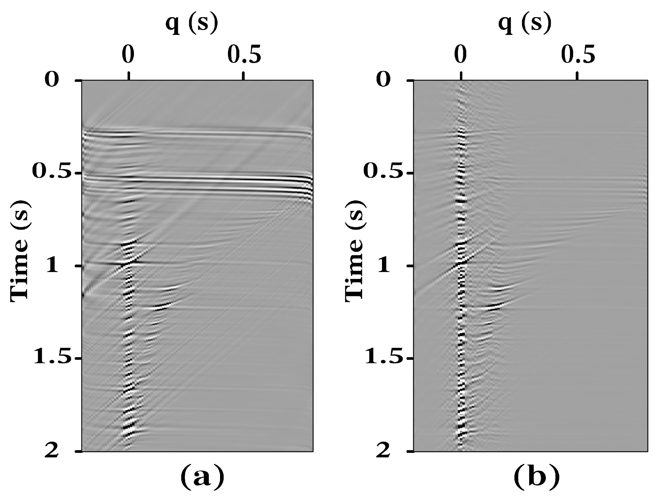
2.2. Geometric Mode Decomposition

Taking inspiration from VMD [18], Yu et al. proposed the geometric mode decomposition (GMD) [21]. GMD considers two-dimensional seismic data as a combination of band-limited modes with line or parabolic geometric features. By iteratively calculating the weighted center of the energy spectrum, GMD can extract modes with different geometric characteristics, such as slopes or curvatures. GMD contains two variants: GMD-F, which performs decomposition in the frequency domain, and GMD-R, which performs decomposition in the Radon domain. In this study, our focus lies on GMD-R as it allows for the suppression of multiples by exploiting the separability of primaries and multiples in the Radon domain. Consequently, the optimization problem is formulated as follows:

$$\underset{u_k,{\beta }_k}{\min }{\displaystyle \sum _{k=1}^{K_m}{\Vert {\partial }_x\mathrm{NMO}(u_k,{\beta }_k)\Vert }_2^2}s.t.{\displaystyle \sum _{k=1}^{K_m}{u}_k}=\widehat{d},$$

(18)

where ${\beta }_k=({\tau }_k,q_k)$ represents the Radon parameter including intercept time ${\tau }_k$ and slowness parameters $q_k$, $u_k$ denotes the k-th decomposed mode, $\widehat{d}$ is the input data, and $K_m$ represents the predefined number of decomposed modes. $\mathrm{NMO}(u_k,{\beta }_k)$ denotes that the NMO correction is implemented to mode $u_k$ and the corrected mode has a Radon parameter ${\beta }_k$. The optimization problem of Equation (18) can be understood in three parts: (1) decomposing the input data into a combination of modes $u_k$ with different Radon parameters ${\beta }_k$; (2) performing NMO correction to the decomposed mode $u_k$; and (3) after NMO correction, minimize the $l_2$ norm of the derivation to ensure the smoothness of $u_k$ along x-axis.

The augmented Lagrangian of Equation (18) is expressed as

$$L\left(u_k,{\beta }_k\right):=\gamma {\displaystyle \sum _{k=1}^{K_m}{\Vert {\partial }_x\mathrm{NMO}(u_k,{\beta }_k)\Vert }_2^2}+{\Vert \widehat{d}-{\displaystyle \sum _{k=1}^{K_m}{u}_k\left({\beta }_k\right)}\Vert }_2^2,$$

(19)

where $\gamma$ represents the balance parameter. The optimization problem of GMD-R is addressed using the ADMM algorithm. The algorithm updates the decomposed modes and Radon parameters through several iterations. The calculation procedure and solution of GMD-R is given and summarized in Algorithm 2 [21].

GMD-R plays a role in clustering signals in the Radon domain. Firstly, we define the number of decomposed modes $K_m$ and randomly initialize several Radon parameters ${\beta }_k$ in the Radon domain according to $K_m$. Then, the updated modes are calculated using Equation (20), which has the form of a Wiener filter function. The shape of Wiener filter is shown in Figure 1, from which we can see that the Wiener filter plays the role of convergence and allows signals to converge more closely to the center Radon coefficients ${\beta }_k$. Therefore, we can achieve the mode decomposition with different Radon coefficients using the Wiener filter. The new Radon parameters ${\beta }_k$ are determined using Equation (21). The iteration will continue computing until the convergence standard is satisfied and the convergent modes ${\widehat{R}}_k$ are finally obtained [21]. By applying the inverse RT to these modes, the corresponding decomposed modes in the time–space domain are obtained. Note that the summation of the decomposed modes is equivalent to the input Radon model $\widehat{m}(\beta )$.

Algorithm 2 The ADMM algorithm for the GMD-R problem
$\mathrm{Input}: \widehat{d},\widehat{m}\left(\beta \right),\gamma ,\epsilon ,K_m,N_{iter}$ $\mathrm{Output}: {\widehat{u}}_k\left(\beta \right)$. $\mathrm{Initialize} {\beta }_k^1=({\tau }_k^1,p_k^1)$$, n=0$$, \widehat{m}\left(\beta \right)$ is the Radon model of input data $\widehat{d}$$, {\widehat{R}}_k$$\mathrm{denotes} \mathrm{the} \mathrm{decomposed} \mathrm{modes} \mathrm{in} \mathrm{the} \mathrm{Radon} \mathrm{domain}, \mathrm{and} N_{iter}$ is the maximum iteration times.
$1: \mathbf{for} n=0:N_{iter}$ do
$2: \mathbf{for} k=1:K_m$ do
$3: \mathrm{update} {\widehat{R}}_k$:
$${\widehat{R}}_k^{n+1}(\beta )=\frac{\widehat{m}(\beta )-{\displaystyle \sum _{i\ne k}{\widehat{R}}_i(\beta )}}{1+2\gamma {\left(\beta -{\beta }_k\right)}^2},$$ (20)
4:      end for
$5: \mathbf{for} k=1:K_m$ do
$6: \mathrm{update} {\beta }_k$:
$${\beta }_k^{n+1}=\frac{{\displaystyle \int {}_{{\beta }_k}\beta {\left|{\widehat{R}}_k(\beta )\right|}^2\mathrm{d}\beta }}{{\displaystyle \int {}_{{\beta }_k}{\left|{\widehat{R}}_k(\beta )\right|}^2\mathrm{d}\beta }},$$ (21)
7:             end for
$8: \mathbf{If}{\displaystyle \sum _k\left({\Vert {\widehat{R}}_k^{n+1}-{\widehat{R}}_k^n\Vert }_2^2\right)}<tol \mathbf{Exit}$	(22)
9: end for

After NMO correction, multiples and primaries exhibit different curvatures and are distributed in the different areas in the Radon domain, which has a certain separability and distinct geometric features. GMD-R uses the Wiener filter to make the primary and multiple modes converge to their center Radon coefficients gradually, and can decompose them from the original Radon model, thus finally achieving the decomposition of the primary and multiple modes. Starting from this perspective, we developed a novel GMD-based processing flow that can automatically achieve the separation of primaries and multiples. Here, we will provide a detailed explanation of how to apply the GMD-R algorithm for multiple suppression. The procedure of the proposed framework can be divided into three steps:

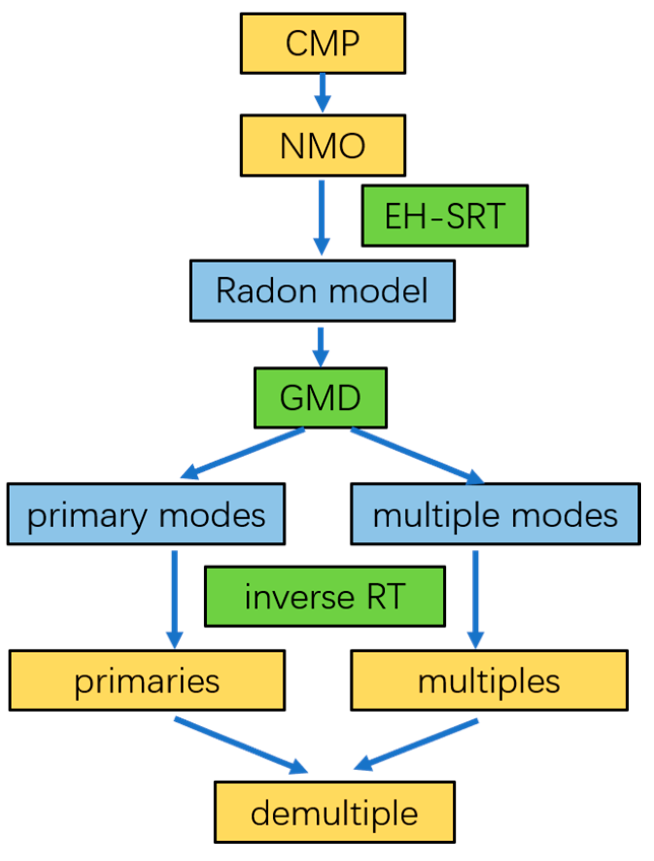
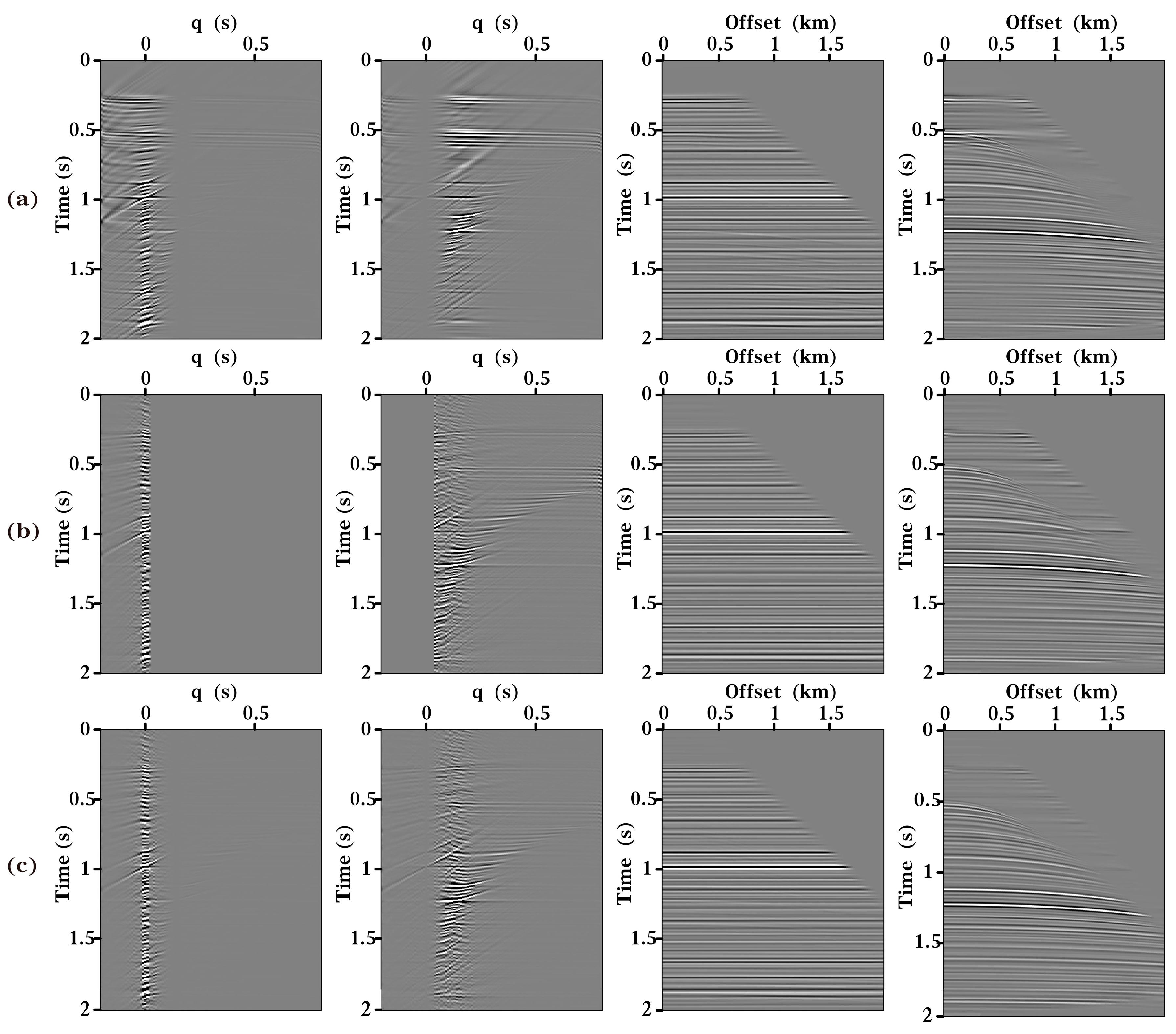
(1)

Apply NMO correction to the input CMP gather data $d$ and then calculate the Radon model $m$ using the LSRT;

(2)

By setting the number of decomposition modes to 2, perform GMD-R to the Radon model $m$ following Algorithm 2 and obtain the separated primary and multiple modes in the Radon domain;

(3)

Perform inverse RT to the separated primary modes and the demultiple result is finally obtained.

The main advantage of the GMD-based demultiple method over the Radon filter method is that it does not require too many parameters to be set artificially. In the GMD procedure, the decomposition of modes is achieved following the algorithm in Algorithm 2, which is an automatic calculation process. From this point, we can separate primary modes and multiple modes because they have different curvatures. Compared with the traditional Radon filter method, there will be no need to set the filtering parameters artificially, which means that it is less affected by human intervention. The only parameter that needs to be set is the number of decomposition modes and we usually set it to 2 for multiple suppression in the second step. The reason will be given in the discussion part, where we will analyze the effect of decomposition number in GMD-R.

2.3. Improve GMD-R with the EH Norm Constraint Sparse Radon Transform

GMD-R enables the decomposition of modes with distinct geometric characteristics. However, when the resolution of the input Radon model is insufficient, it can result in an overlap between multiples and primaries in the Radon domain, which reduces the effectiveness of mode decomposition. Moreover, the Radon model with low sparsity requires a substantial number of iterative calculations by GMD-R to ensure that the separated mode reaches convergence. To overcome these issues, the EH-SRT is introduced to improve the GMD-based multiple removal framework. The processing flow of the improved GMD-based demultiple framework is shown in Figure 2. Here, the yellow box represents the data in the time-offset domain, while the blue box represents the data in the Radon domain. The green box denotes the calculation procedures, including the EH-SRT, GMD and the inverse RT. Here, we replace the LSRT with the EH-SRT to perform the RT. The use of EH-SRT yields a Radon model with higher sparsity and stronger separability between primaries and multiples. This enhancement aids the GMD-R method in effectively separating multiple and primary modes. Moreover, the Radon model with high sparsity simplifies the convergence process during the GMD-R decomposition. Based on this, the combination of EH-SRT and GMD-R can not only achieve better separation of primary and multiple modes but also improve the computational efficiency of GMD-R.

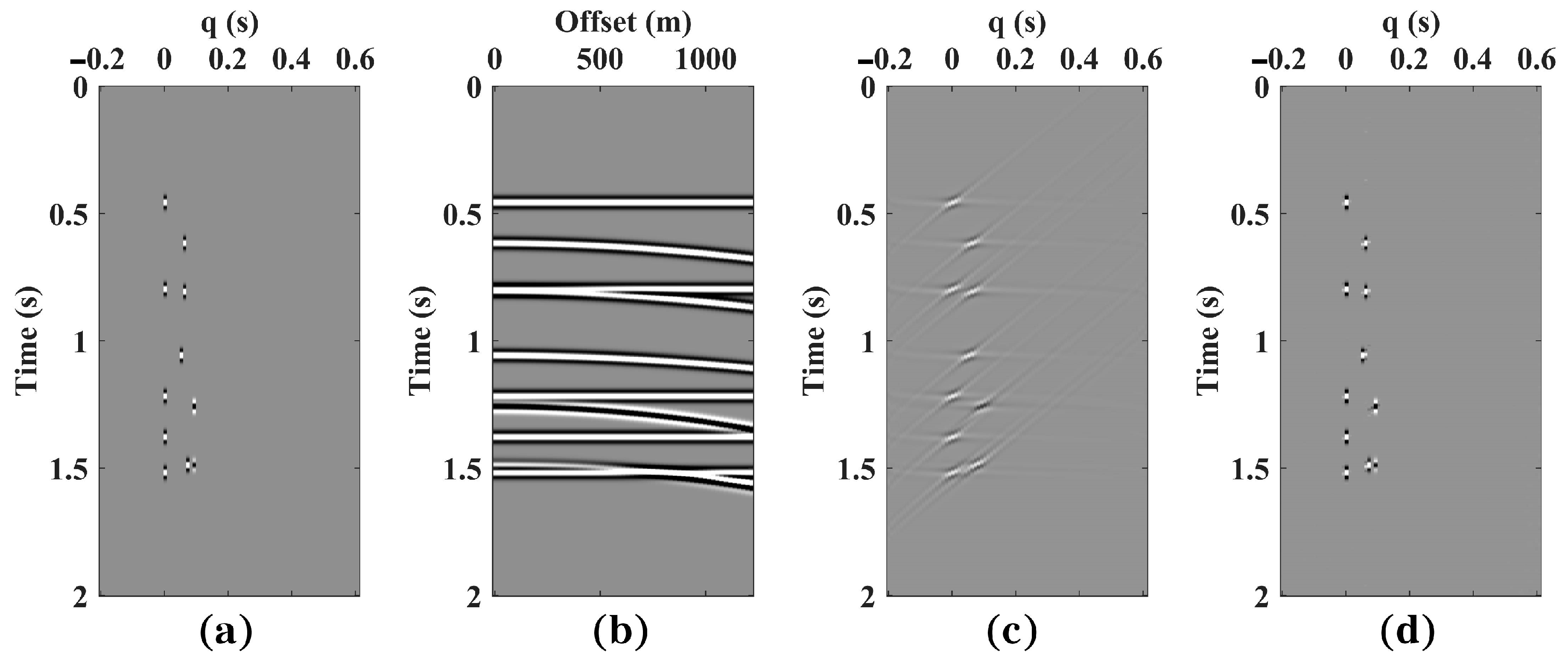
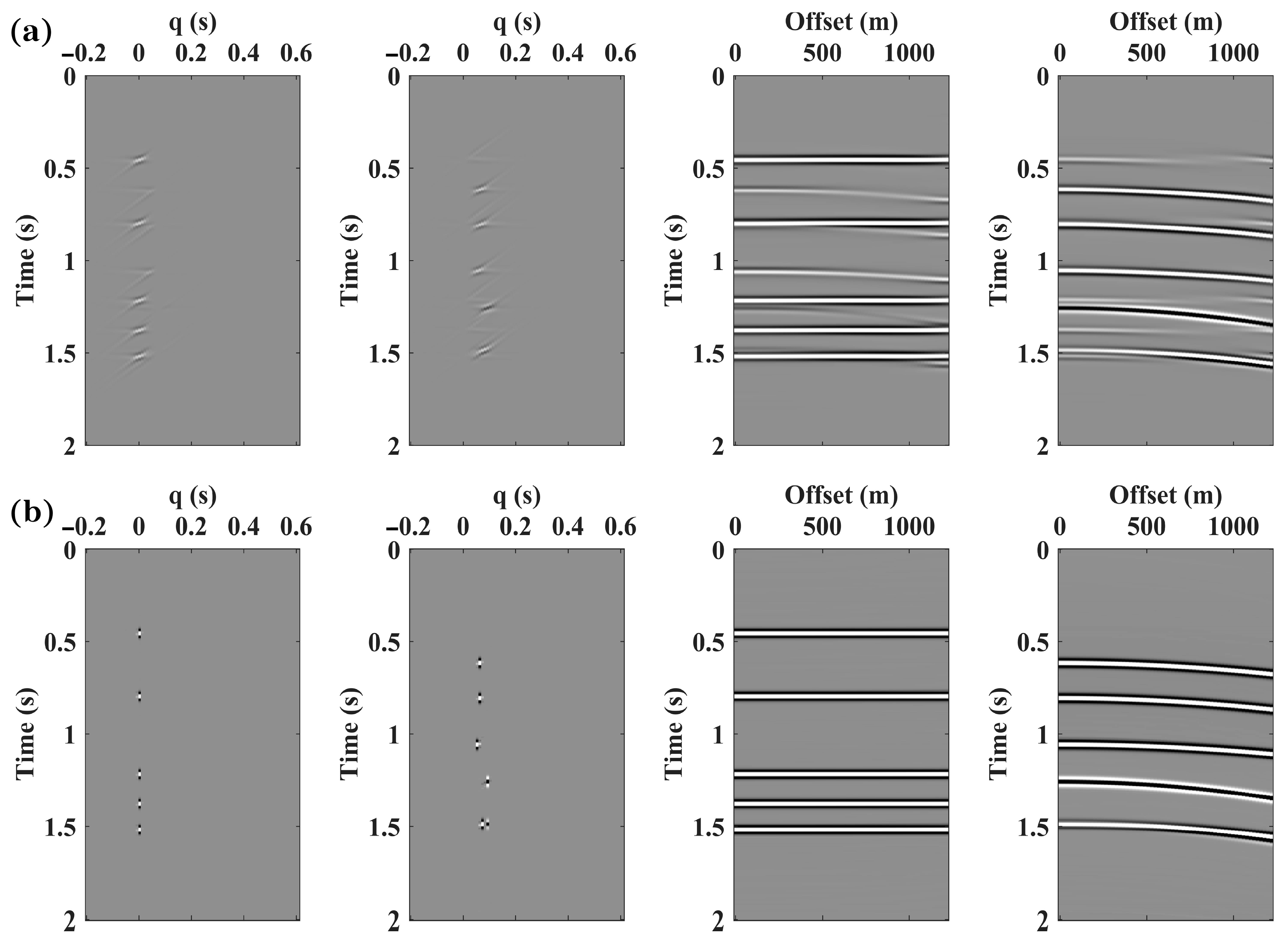
3. Numerical Examples

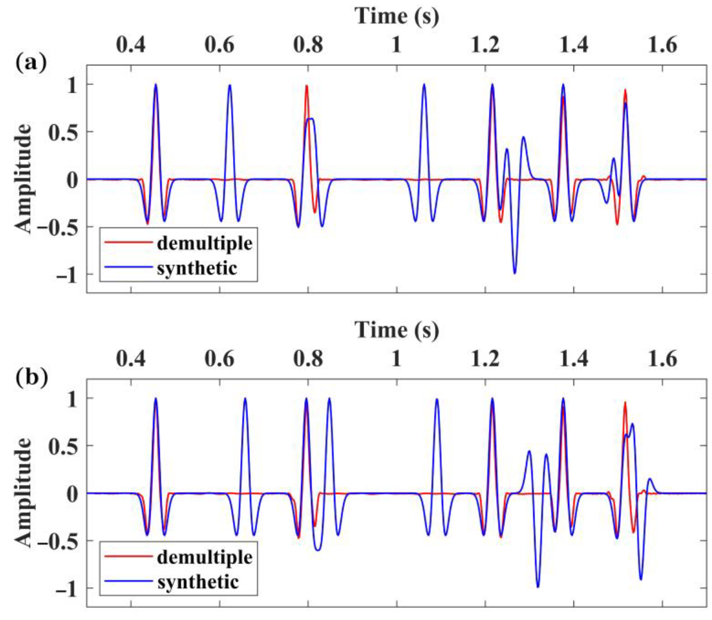
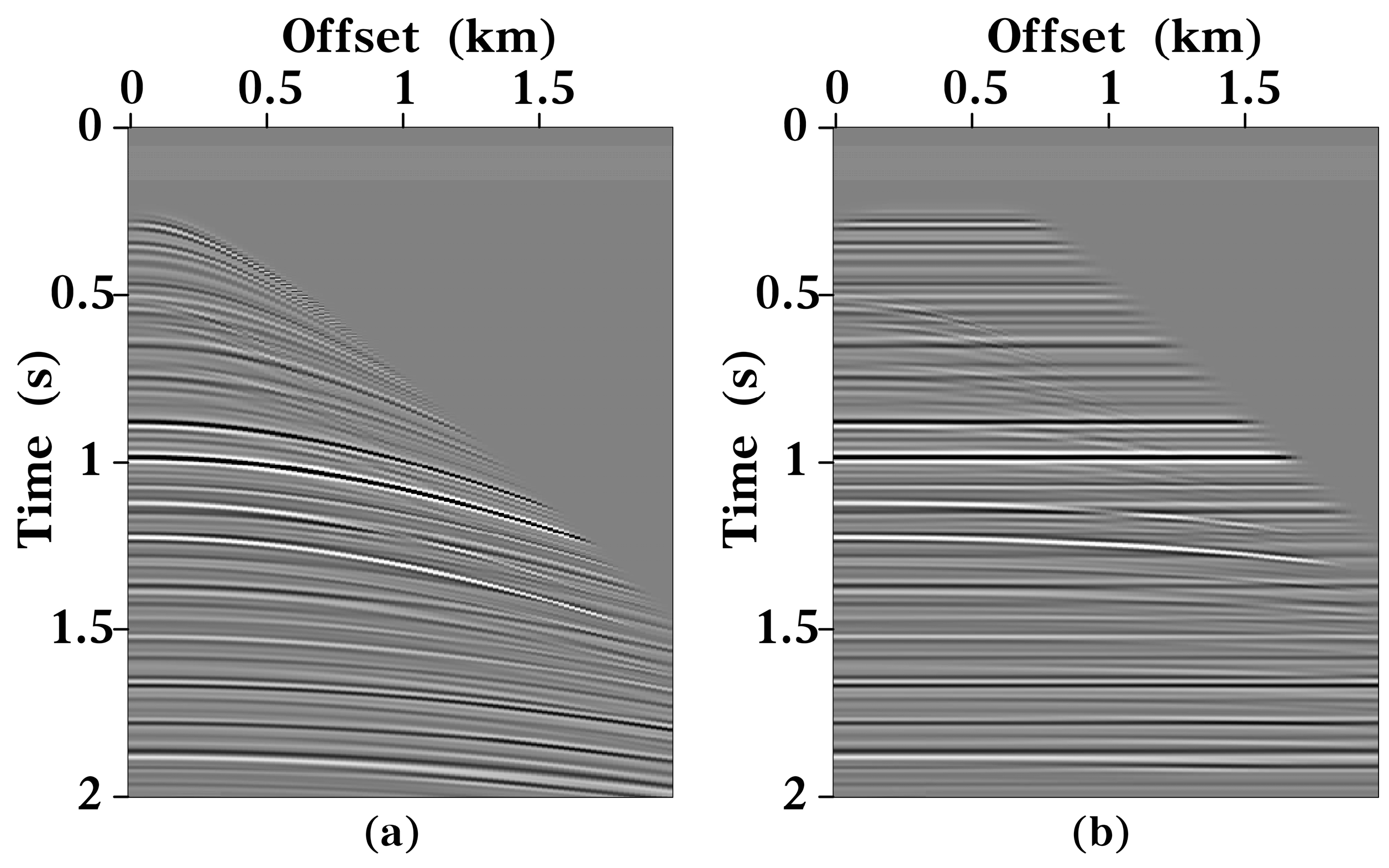
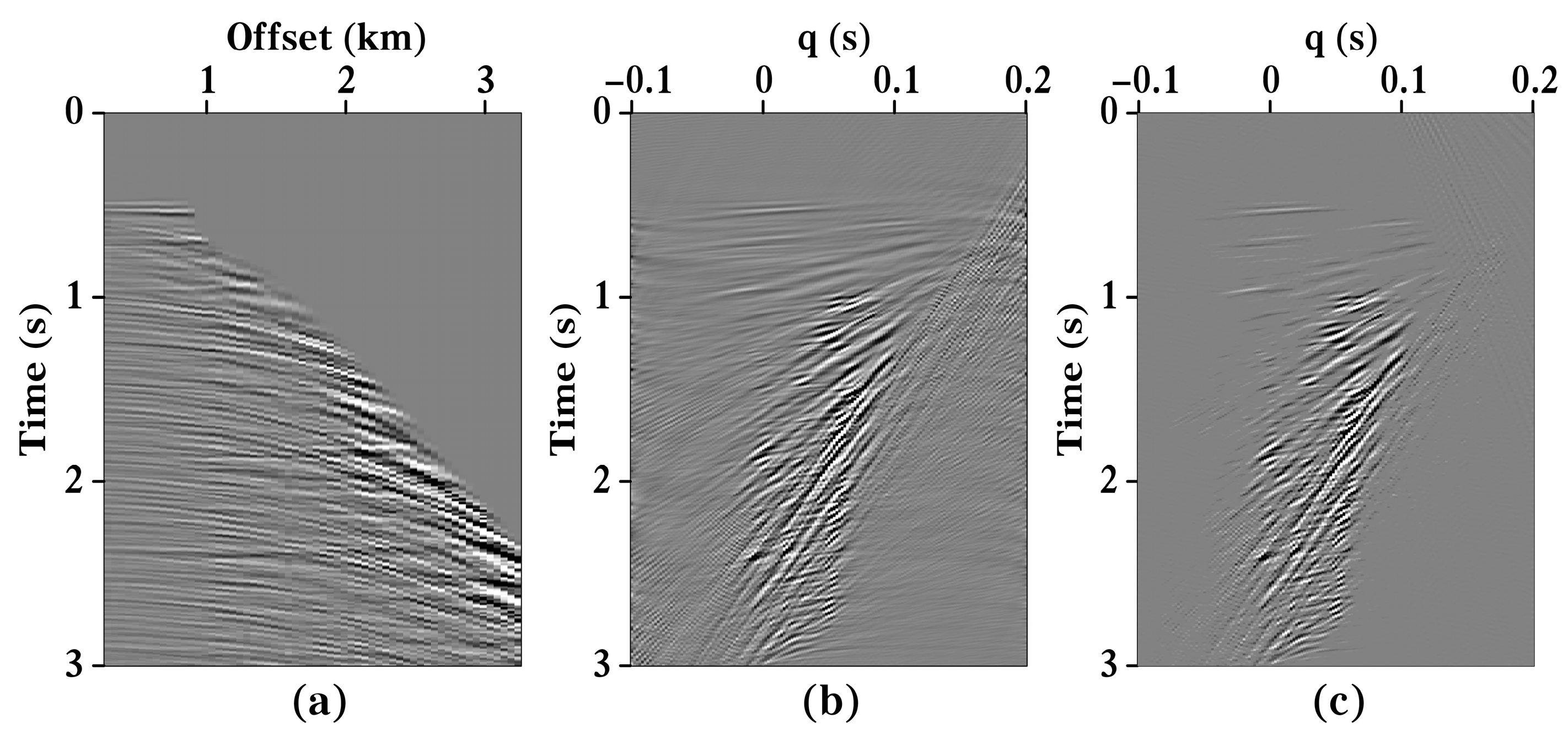
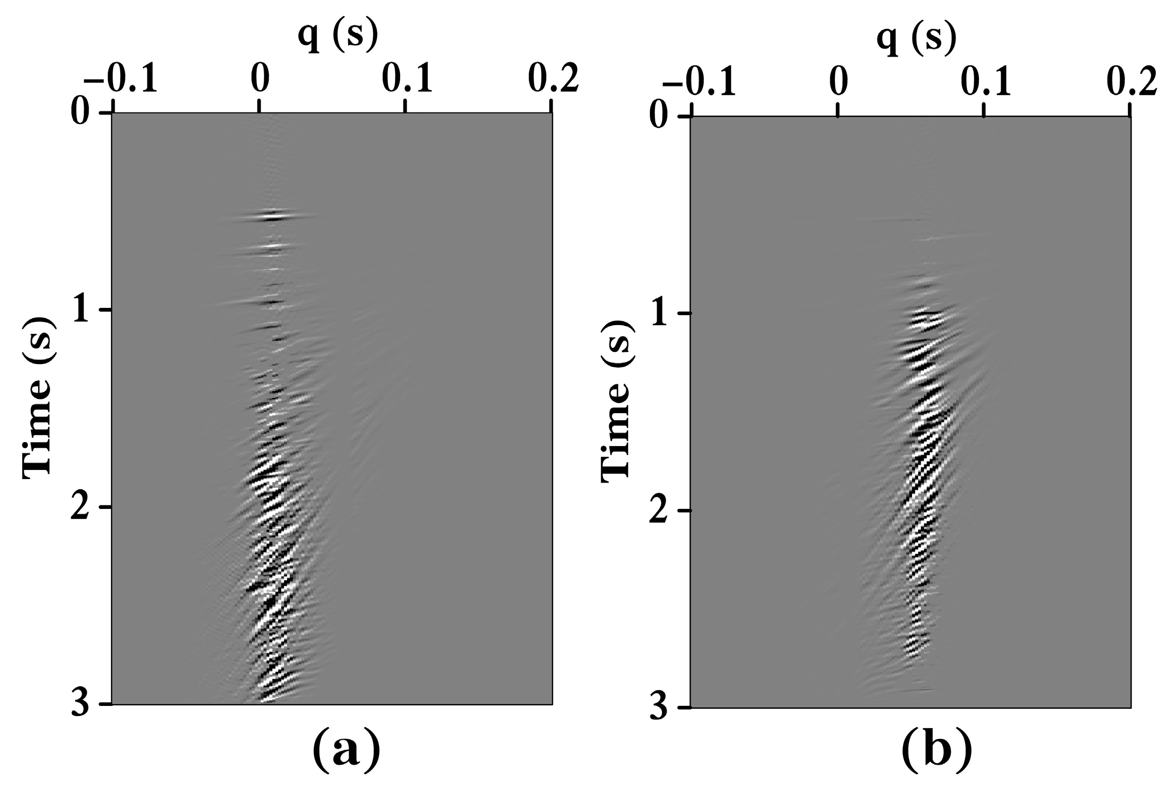
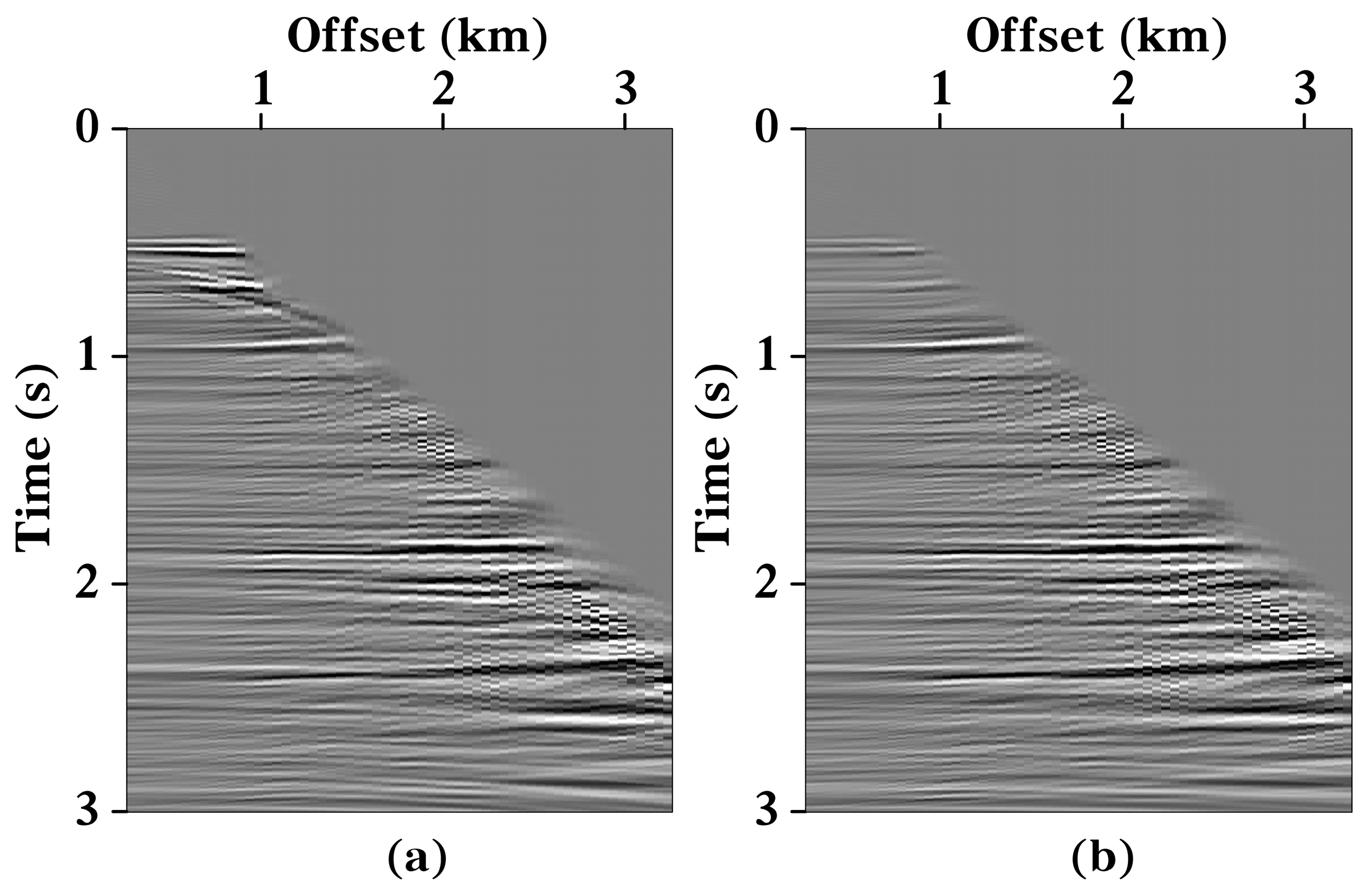
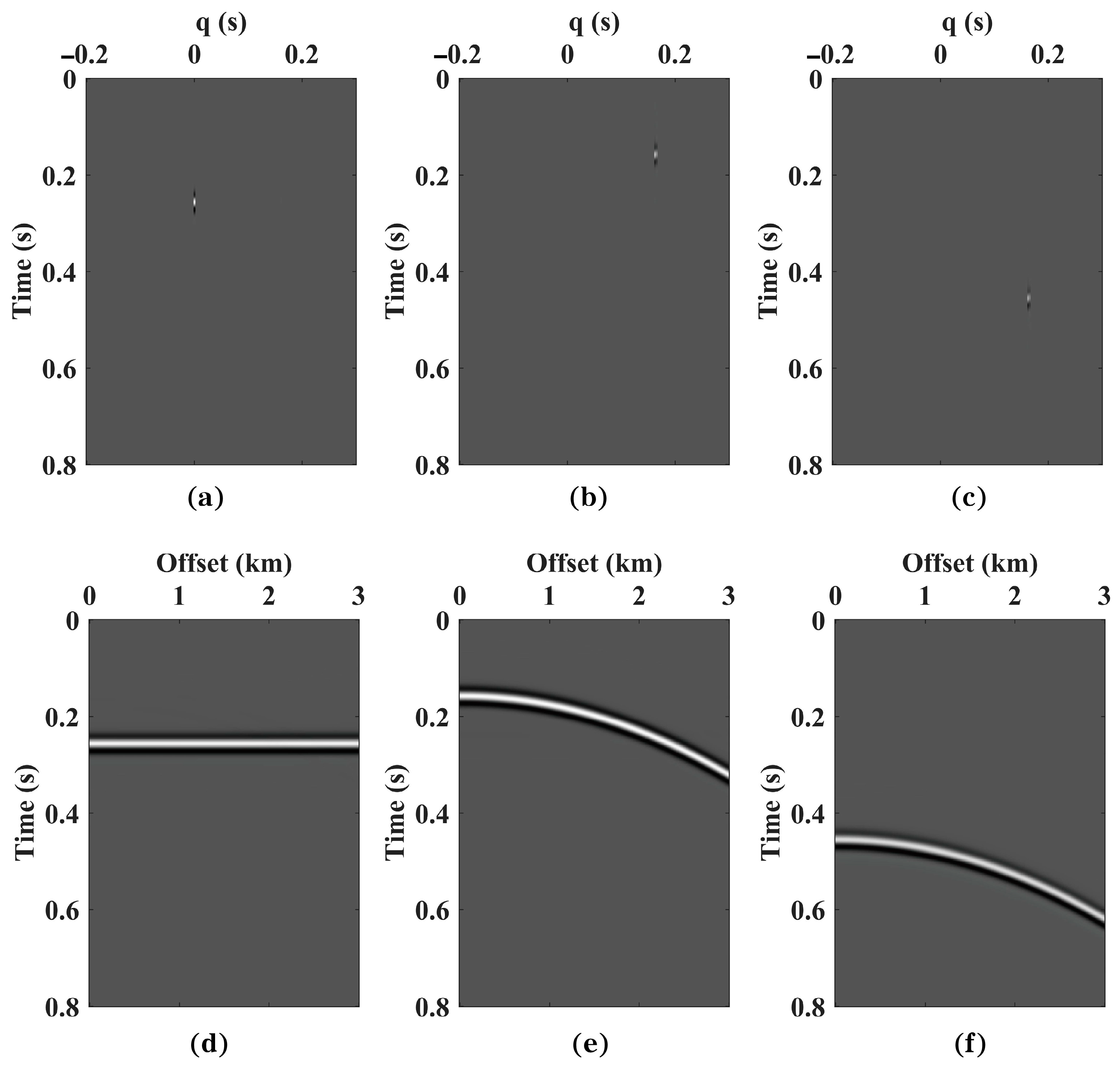
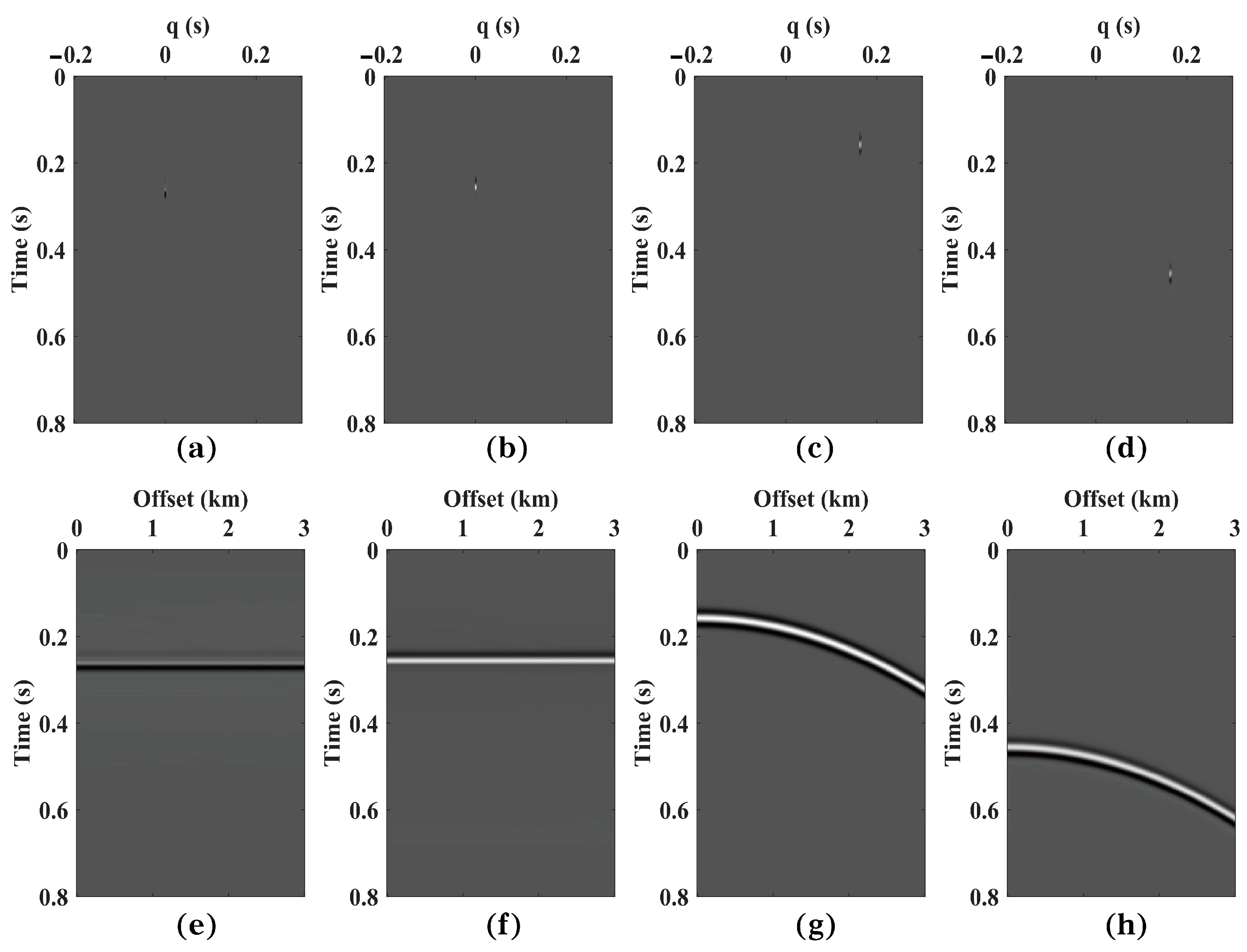
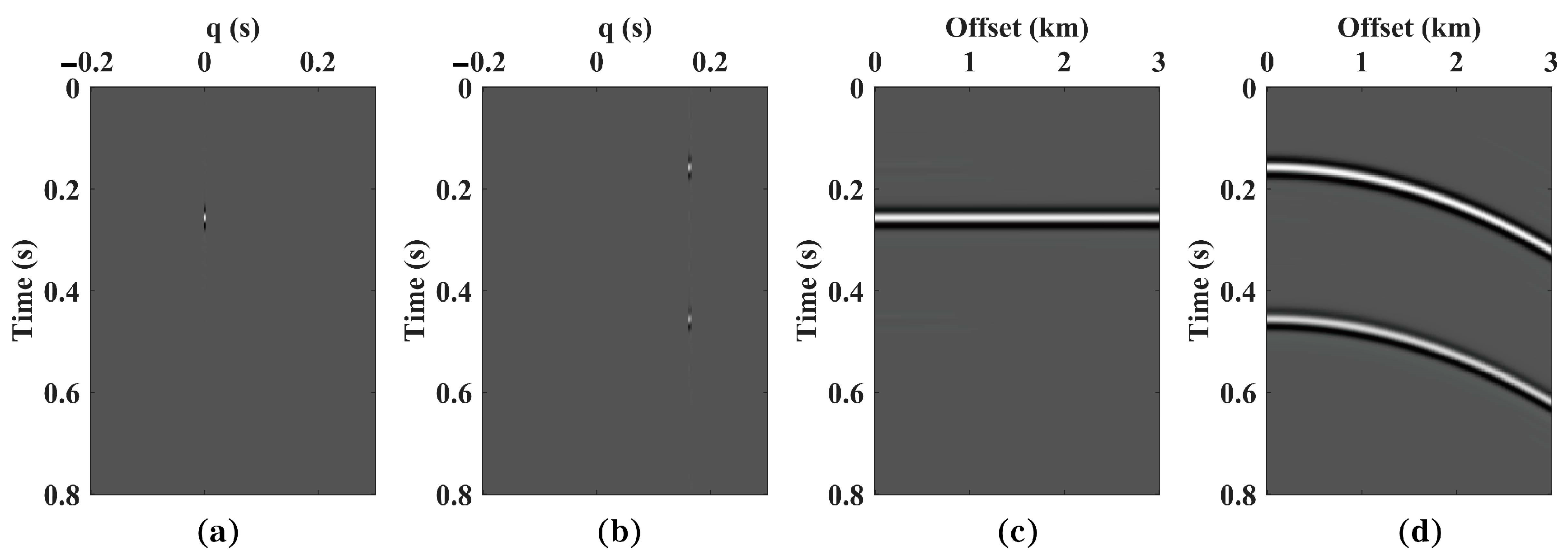
3.1. Synthetic Data 1 Test

In this section, we design a Radon model consisting of five primaries and several multiples as shown in Figure 3a, and its synthetic data are displayed in Figure 3b. The size of the synthetic data is set as 1001 × 60, with a sampling interval of 2 ms and a trace interval of 20 m. The Radon coefficients of primaries in the true Radon model are located in the line where its horizontal ordinate is $q=0$, and the multiple coefficients are distributed in the area where $0.04\le q\le 0.1$. Figure 3b displays the fact that multiples and primaries exhibit superposition at near offset and cross-over at far offset in the synthetic data. To demonstrate the effectiveness of our proposed EH-SRT, we perform LSRT and EH-SRT to the synthetic data, and the estimated Radon models are displayed in Figure 3c,d. It is apparent that the Radon model of LSRT is not sparse, causing primaries and multiples to overlap with each other. While the Radon model of EH-SRT is very sparse and is very similar to the true Radon model.

Subsequently, GMD-R is applied to the two Radon models to decompose modes, which are displayed in Figure 4a,b. The four columns in Figure 4 represent the decomposed primary modes, the decomposed multiple modes, the recovered primaries, and the recovered multiples, respectively. One can find from Figure 4a that the decomposition results of the LSRT model are unsatisfactory due to limited sparsity of the LSRT model. There are multiple coefficients in the separated primary modes, resulting in multiple residuals in the recovered primaries. While these issues are fixed in the decomposition results of the EH-SRT model, multiples and primaries are separated not only in the Radon domain but also in the time domain. And there are no residual multiples in the recovered primaries.

To more clearly verify the effectiveness of the proposed approach in multiple removal, we select a near-offset trace at $x=420$ m and a far-offset trace at $x=1020$ m to conduct the amplitude comparison before and after multiple elimination. It is crucial to note that only the demultiple result based on the EH-SRT model is employed in this test. In Figure 5a, the amplitude comparison of the near-offset trace is presented, where the blue line represents the amplitude of the synthetic data, and the red line represents the amplitude of the recovered primaries. It is apparent that there are obvious multiples at 0.6 s, 1.05 s, and 1.25 s, while the multiples at 0.8 s and 1.5 s are not easily discovered. This is because multiples overlap with primaries, leading to waveform variations in both types of reflections. Through comparison, it can be observed that GMD-R can not only suppress the obvious multiples but also recover primaries affected by multiples at 0.8 s and 1.5 s. This achievement can be attributed to the precise separation of primary and multiple coefficients achieved in the Radon domain. The far-offset trace comparison is displayed in Figure 5b, where multiples exhibit a certain time shift compared with Figure 5a. The waveform variations in Figure 5b reaffirm the conclusion drawn from Figure 5a, highlighting the ability of GMD-R to effectively suppress multiples and recover primary signals.

3.2. Synthetic Data 2 Test

In this section, a complex synthetic data with several multiples are generated to further verify the method’s efficiency. Figure 6a,b show the designed synthetic CMP data before and after the NMO correction. It is apparent that multiples have a parabolic shape and are more easily to detect after the NMO correction. The size of the synthetic data is set as 1001 × 100, with a sampling interval of 2 ms and a trace interval of 20 m.

We perform the LSRT and EH-SRT to the NMO-corrected data and the estimated Radon model is shown in Figure 7a,b, respectively. The Radon model has the same time sampling and interval with seismic gather, with 101 slowness sampling points ranging from −0.2 to 0.8. It is apparent in Figure 7a that the Radon model of the LSRT is divergent in shallow layers, which is caused by the stack of limited traces after muting the NMO stretching [25], while the Radon model of EH-SRT is sparser than the LSRT result not only in the low layers but also in the deep region. The velocity for NMO correction is known to be absolutely accurate, resulting in the correction of primaries from parabolic to flat. Consequently, the Radon coefficients of the primary are aligned along a line where its horizontal ordinate is $q=0$. However, the Radon coefficients of multiple vary with depth and slowness, and the deeper the layer is, the closer the Radon coefficients of multiples are to primaries.

To verify the help of the EH-SRT to GMD-R, we apply GMD-R to the Radon model of LSRT and EH-SRT, and the result is shown in Figure 8a,c, respectively. The four columns in Figure 8 represent the separated primary modes, the separated multiple modes, the recovered primaries by performing the inverse RT to the decomposed primary modes, and the suppressed multiples. It is important to note that the fourth column does not represent the recovered multiples achieved by performing the inverse Radon transform on the separated multiple modes. Instead, it is the suppressed multiples obtained by subtracting the recovered primaries from the synthetic data. Comparing Figure 8a,c, we can observe that GMD-R achieves the separation of multiple and primary modes for both the LSRT and EH-SRT models. The decomposed primary modes entirely keep the linear features of primary coefficients in the Radon domain. However, due to the sparsity of the Radon model, the primary modes separated from the LSRT model contain many multiple Radon coefficients. As a result, some residual multiples are present in the recovered primaries. Meanwhile, in the shallow region, due to the lack of convergence of the LSRT model, there are many primary Radon coefficients decomposed in the multiple modes, leading to amplitude attenuation of the recovered primaries. The leakage of primaries in the difference profile indicates the issues. In contrast, these problems are greatly reduced in the EH-SRT processing result. It can be seen from the residual profile in Figure 8c that the recovered primary amplitudes in the shallow layers are less damaged.

To further demonstrate the superiority of the GMD-based method over the filter method, we also applied the filter method to the EH-SRT model to suppress multiples. After several filtering parameter adjustments, the best multiple suppression results are obtained when the Radon coefficients with $q>0.05$ are taken as multiples and muted, and the result is shown in Figure 8b. The four columns in Figure 8b represent the retained primary Radon coefficients, the muted multiple Radon coefficients, the recovered primaries, and the differences between the recovered primaries and the synthetic data. From the difference profile, it is evident that the filter method effectively suppresses multiples. However, as a drawback, some of the primary coefficients are unintentionally suppressed as well. This excessive suppression of multiples leads to damage to primaries. There are fewer primary residuals in the difference panel in Figure 8c, which shows the advantage of GMD-R in preserving primaries. Instead of directly cutting off to separate primaries and multiples in the filter method, GMD-R uses a Wiener filter to cluster and separate modes. By gradually decaying the modes within the Radon domain at the boundary, GMD-R avoids the truncation effect, allowing for better recovery of the primaries while maintaining their amplitude.

In this synthetic dataset, it would not be scientifically rigorous to compare amplitude variation before and after multiple suppression with only one trace. Therefore, a single trace, which is generated by superimposing 20 traces in the range from 0 to 500 m, is used to showcase the amplitude variation. Figure 9 displays the stacked trace, in which the black line represents the amplitude of synthetic data, and the red line and blue line indicate the recovered primaries with the Radon filter method and the GMD-R method, respectively. To provide a reference for comparison, the green line represents the stacked trace obtained by integrating synthetic data without multiples. This serves as a means to demonstrate the abilities of the two methods in preserving amplitude and suppressing multiples. It is evident that after multiple suppression, the amplitude at 1.12 s, 1.22 s, and 1.38 s decreased, but the amplitude of the GMD-R result is closer to the multiple-free data, validating the superior multiple suppression capability of GMD-R. Additionally, the demultiple result obtained with GMD-R showcases similar amplitudes as the multiple-free data at other times, further supporting the claim that GMD-R effectively preserves the amplitude of the primary signals. A conclusion can be drawn from the test that the proposed GMD-R can not only achieve a better multiple removal than the filtering method but also preserve the amplitude of primaries.

Multiples in seismic data exhibit low velocities compared to primaries, and they show different patterns in the velocity scanning spectrum. Therefore, we can evaluate the effectiveness of the two demultiple methods through velocity scan analysis. We perform velocity scanning to the synthetic data in Figure 6a and the velocity spectrum is shown in Figure 10a. One can find from the velocity spectrum that in addition to the primary energy clusters, which are linearly increasing with depths, that there are several low-velocity multiple energy clusters. Then, we perform velocity scanning to the demultiple result of the Radon filter method and GMD-R in Figure 8b,c, and the velocity spectrum is displayed in Figure 10b,c, respectively. Note that before velocity scanning, the multiple suppression result in Figure 8 is processed with the inverse NMO correction. It is evident that the multiple energy clusters in the velocity spectrum of raw synthetic data are both significantly reduced in Figure 10b,c. The reduced multiple energy clusters are primarily at 1.12 s, 1.22 s, and 1.38 s, which aligns with the findings presented in Figure 9. Moreover, the primary energy clusters of the demultiple result from GMD-R are more converged and focused, providing additional evidence for the efficacy of the proposed method in suppressing multiples and preserving primary amplitude.

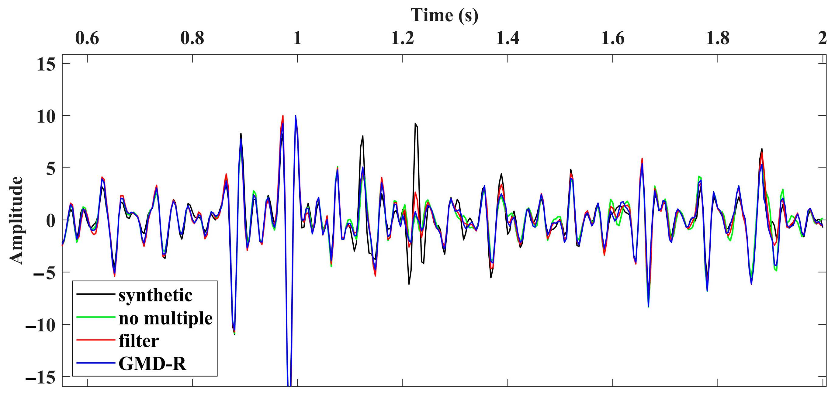
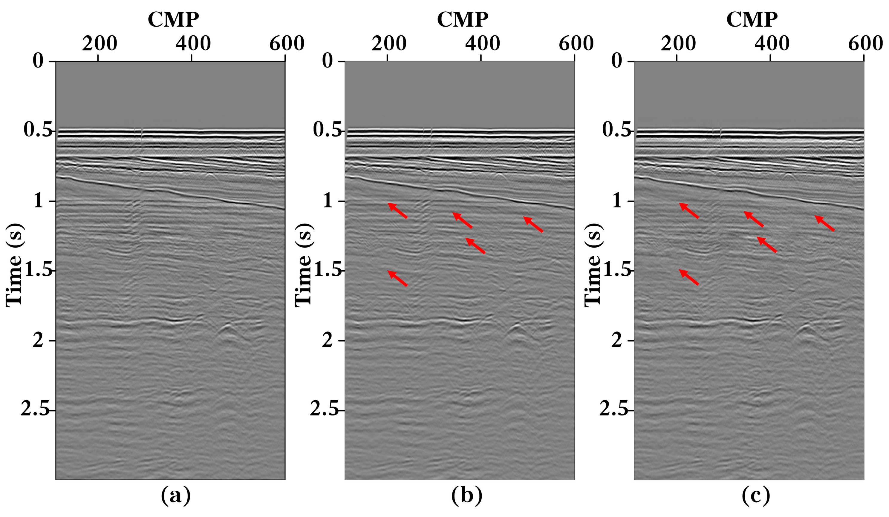
3.3. Field Data Test

The practicality of the proposed approach is showcased in this section through the utilization of field data obtained from the open-source Madagascar. A CMP gather from the dataset is selected and shown in Figure 11a, and there are 751 time samplings and 60 traces, with a sampling interval of 4 ms and a trace interval of 50 m. We perform the LSRT and EH-SRT to the data and the estimated Radon model is shown in Figure 11b,c, respectively. The Radon model has the same time sampling and interval as the field data and with 161 slowness sampling points ranging from −0.1 to 0.2. And there are numerous artifacts in the LSRT model in Figure 11b, which are caused by the stack of limited traces after muting the NMO stretching. It is apparent that the Radon model obtained by EH-SRT is sparser and has fewer artifacts than the LSRT result.

Next, we perform GMD-R on the Radon model of EH-SRT. Figure 12a,b shows the decomposed primary modes and multiple modes, respectively. It is evident that the separated primary modes are mainly focused around the vicinity of slowness $q=0$, and the multiple modes are out of the area, thus achieving the separation of primaries and multiples. And then we perform the inverse RT to the primaries modes and the recovered primaries are shown in Figure 13b. One can find that there are fewer multiples in the multiple elimination result of the GMD-R method. And then, the filter method is applied to the EH-SRT model to suppress multiples. After several tests, the optimal demultiple result is obtained when the Radon coefficients in the region of horizontal coordinates $q>0.015$ and vertical coordinates $t>0.7 s$ are taken as multiple and muted. After that, by performing the inverse RT to the filtered Radon model, the demultiple result is obtained and shown in Figure 13a.

We then perform inverse NMO correction to the demultiple result of the two methods in Figure 13. Subsequently, we conducted velocity scanning analysis to generate the velocity spectrum, as shown in Figure 14b,c. In the velocity spectrum of the raw data, as shown in Figure 14a, the velocity energy clusters mainly locate in the low-velocity region, which is due to the presence of the relatively low-velocity multiples in the field data. After multiple removal, these energy clusters in the low-velocity region significantly decrease, while the energy clusters of primaries become clear and exhibit a characteristic increase with depth. In comparison to the filter method, the primary energy clusters in Figure 14c are more focused, and exhibit fewer low-velocity residuals, indicating the advantage of the GMD-R method in multiple removal.

Figure 15a–c shows the stack profile of the raw data, the demultiple result of the filter method and GMD-R method, respectively. Compared with the stack profile before multiple elimination, the filter method and GMD-R method both suppress several multiples. However, there are still some multiple residuals in Figure 15b while these multiples are absent in Figure 15c, especially in the areas pointed by the red arrows. From this point, we can recognize that the proposed method obtains a better result in multiple suppression.

4. Discussion

4.1. The Effect of the Number of Decomposed Modes

Similar to EMD and VMD, the number of decomposed modes is a crucial parameter in GMD and must be accurately determined before processing. Setting the number of modes too high can lead to unnecessary computational overhead or the destruction of effective modes, while setting it too low can result in an incomplete decomposition of the modes. In this section, we present a simple example to demonstrate how to select the appropriate number of decomposed modes in GMD-R.

Figure 16a depicts a synthetic seismic dataset containing a horizontal event and two parabolic events with similar curvature. We perform the LSRT and the EH-SRT to the synthetic data and the two estimated Radon models are displayed in Figure 16b,c, respectively. One can find that the Radon model of our proposed method exhibits a higher sparsity and contains fewer Radon coefficients compared to the LSRT result.

Then, GMD-R with different decomposition numbers is applied to the EH-SRT Radon model to show the effect of the decomposition number selection. First, we perform GMD-R to the Radon model of EH-SRT with a decomposition number of three. Figure 17 showcases these decomposed modes, with the top row presenting the modes in the Radon domain, and the bottom row showing the three corresponding recovered events in the time domain. It is evident from Figure 17 that the three events in Figure 16a are taken as three modes and separated. Next, we repeat the same processing for Figure 16a, but this time with a decomposition number of four. Figure 18 depicts the result, with the top row indicating the four decomposed modes in the Radon domain and the bottom row displaying the four recovered events corresponding to the top row data. It can be observed that the first mode in Figure 17 is split into two modes in Figure 18 because the decomposition number exceeds the actual number of modes. The effectively separated modes are corrupted by the excessive decomposition number. In addition, we perform the same processing with a decomposition number of two, and the result is shown in Figure 19. The two decomposed Radon modes are displayed in Figure 19a,b, while Figure 19c,d present the recovered events corresponding to Figure 19a,b. Figure 19 illustrates that the flat event is treated as one mode, whereas the other two parabolic events are considered as one mode due to their similar curvature. Conclusions can be drawn from this test that what GMD-R focuses more on is curvature, not intercept time.

In seismic processing, if the velocity is corrected, primaries are horizontal while multiples are not horizontal after NMO correction. The two types of reflection waves can be represented as $q=0$ and $q>0$ in the Radon domain. Therefore, we can apply GMD-R to the NMO-corrected gather to separate primary and multiple modes by selecting the decomposition number of 2.

4.2. The Computational Efficiency of the ES-SRT and GMD

A processing method should not only consider the quality of its processing results but also the calculation time and efficiency. We analyze the computational efficiency of the EH-SRT and GMD-R here. Taking the synthetic data in Section 3.2 as an example, we record the computation time of performing the LSRT and EH-SRT to the data and the time of GMD-R decomposition on these two Radon models.

Table 1. Computation time comparison of the LSRT and EH-SRT, and performing GMD on the two Radon models.

Test Data	Method	Computation Time (s)	Method	Computation Time (s)
Synthetic data 2	LSRT	1.08	GMD-R	2.17
	EH-SRT	3.56	GMD-R	1.32

shows the statistical time. Table 1 shows that the proposed EH-SRT is a little slower than the LSRT because there are several iterations required in the procedure. However, the method can obtain a higher sparsity Radon model, which can be used not only for GMD-R decomposition but also helpful for the filter method for multiple elimination. Therefore, we consider this increased computational effort acceptable [40,41]. Then, we perform GMD-R to the Radon model of LSRT and EH-SRT, respectively, and the decomposition on the EH-SRT model exhibits a shorter computation time. This is because the increasing sparsity of the Radon model makes the modes in GMD-R easier to reach convergence during the iteration process, and hence accelerate the computation. Therefore, we suggest performing sparse RT first to obtain the Radon model with high sparsity, which not only can achieve better separation of primaries and multiples but can also improve the computational efficiency of GMD-R.

Another important point to note is that both the GMD-based method and the filtering method are implemented in the Radon domain. The RT is the kernel of the proposed method for multiple suppression. However, the RT depends on the quality of the original seismic data. When the trace interval of the input data is large, the Radon model tends to have aliasing issues, and the sparsity is low. Although the sparse Radon transform proposed in this paper can improve its sparsity, it is difficult to solve the aliasing problem, which affects the processing results of this method [25]. In addition, the reason why the RT can be used for multiple removals is that multiples and primaries have a certain separability in the Radon domain due to their differences in curvature. Short-period multiples do not have obvious moveout differences with primaries due to their short propagation paths, so it is difficult to suppress them with the Radon-based multiple suppression method. In the field data test in Section 3.3, we do not suppress free-surface multiples in advance, and the GMD-based method has limited ability to suppress them. Therefore, there are several remaining free-surface multiples in the stack profile at 2.4 s. In the industry, it is customary to employ techniques such as SRME and MWD [42,43,44] as an initial step to suppress free-surface multiples, and then the remaining long-period multiples are suppressed using the Radon-based methods. Multiple elimination cannot be completely solved by one method, and a combination of methods is needed to achieve better suppression results. The method proposed in this paper aims to simplify the processing flow by reducing the parameter setting and complementing other methods for better elimination of multiples.

5. Conclusions

In this paper, to address the issue that the Radon filter method for multiple suppression requires human setting of filtering parameters, a novel framework that can automatically separate multiples and primaries using GMD-R in the sparse Radon domain is proposed. First, GMD-R is introduced and applied to separate multiple and primary modes in the Radon domain. The GMD-R leverages the principle of Wiener filtering to iteratively decompose the data into modes with varying curvature and intercept, thus achieving the separation of primary modes and multiple modes according to their curvature differences. Based on the GMD-R algorithm, we develop a new processing flow for suppressing multiples. Then, we introduce the EH norm as a constraint and propose a novel sparse Radon transform. The EH norm adds an additional scaled $l_2$ norm to the $l_{1/2}$ norm, which is added to overcome the numerical oscillation problem. With the help of the EH norm, the new proposed sparse RT has a higher sparsity and stable solution. Finally, by combining the sparse Radon model, we improve the GMD-based multiple removal framework. Two synthetic data tests and a field data test are employed to illustrate the effectiveness of the proposed framework. The results indicate that the GMD-based framework can achieve the suppression of multiples with a high computational efficiency and can be applied in the actual production. Moreover, it reduces the dependence on manual setting parameters and simplifies the processing flow for multiple elimination.

References

- Yilmaz, Ö. Seismic Data Processing: Processing, Inversion, and Interpretation of Seismic Data; Society of Exploration Geophysicists: Houston, TX, USA, 2008; ISBN 978-1-56080-094-1. [Google Scholar]
- Zhang, Y.; Liu, Y.; Yi, J. Least-Squares Reverse-Time Migration of Water-Bottom-Related Multiples. Remote Sens. 2022, 14, 5979. [Google Scholar] [CrossRef]
- Bruno, P.P.G. Seismic Exploration Methods for Structural Studies and for Active Fault Characterization: A Review. Appl. Sci. 2023, 13, 9473. [Google Scholar] [CrossRef]
- Malehmir, A.; Durrheim, R.; Bellefleur, G.; Urosevic, M.; Juhlin, C.; White, D.J.; Milkereit, B.; Campbell, G. Seismic Methods in Mineral Exploration and Mine Planning: A General Overview of Past and Present Case Histories and a Look into the Future. Geophysics 2012, 77, WC173–WC190. [Google Scholar] [CrossRef]
- John, B.; Diebold; Paul, L. Stoffa The Traveltime Equation, Tau-Rho Mapping and Inversion of Common Midpoint Data. Geophysics 1981, 46, 238–254. [Google Scholar] [CrossRef]
- Trad, D.; Ulrych, T.; Sacchi, M. Latest Views of the Sparse Radon Transform. Geophysics 2003, 68, 386–399. [Google Scholar] [CrossRef]
- Wang, B.; Wang, J.; Li, J.; Guo, Z. Iterative Accurate Seismic Data Deblending by ASB-Based Robust Sparse Radon Transform. IEEE Trans. Geosci. Remote Sens. 2021, 60, 5902309. [Google Scholar] [CrossRef]
- Xue, Y.; Man, M.; Zu, S.; Chang, F.; Chen, Y. Amplitude-Preserving Iterative Deblending of Simultaneous Source Seismic Data Using High-Order Radon Transform. J. Appl. Geophys. 2017, 139, 79–90. [Google Scholar] [CrossRef]
- Zhang, L.; Wang, Y.; Zheng, Y.; Chang, X. Deblending Using a High-Resolution Radon Transform in a Common Midpoint Domain. J. Geophys. Eng. 2015, 12, 167–174. [Google Scholar] [CrossRef]
- Kabir, M.M.N.; Verschuur, D.J. Restoration of Missing Offsets by Parabolic Radon Transform1. Geophys. Prospect. 1995, 43, 347–368. [Google Scholar] [CrossRef]
- Trad, D.O.; Ulrych, T.J.; Sacchi, M.D. Accurate Interpolation with High-Resolution Time-Variant Radon Transforms. Geophysics 2002, 67, 25–26. [Google Scholar] [CrossRef]
- Verschuur, D.J. Seismic Multiple Removal Techniques: Past, Present and Future (EET 1); Earthdoc: Houten, The Netherlands, 2013; ISBN 978-90-73834-96-5. [Google Scholar]
- Foster, D.J.; Mosher, C.C. Suppression of Multiple Reflections Using the Radon Transform. Geophysics 1992, 57, 386–395. [Google Scholar] [CrossRef]
- Han, J.; van der Baan, M. Empirical Mode Decomposition for Seismic Time-Frequency Analysis. Geophysics 2013, 78, O9–O19. [Google Scholar] [CrossRef]
- Gómez, J.L.; Velis, D.R. A Simple Method Inspired by Empirical Mode Decomposition for Denoising Seismic Data. Geophysics 2016, 81, V403–V413. [Google Scholar] [CrossRef]
- Huang, N.E.; Shen, Z.; Long, S.R.; Wu, M.C.; Shih, H.H.; Zheng, Q.; Yen, N.C.; Tung, C.C.; Liu, H.H. The Empirical Mode Decomposition and the Hilbert Spectrum for Nonlinear and Non-Stationary Time Series Analysis. Proc. Math. Phys. Eng. Sci. 1998, 454, 903–995. [Google Scholar] [CrossRef]
- Han, J.; Baan, M.V.D. Empirical Mode Decomposition and Robust Seismic Attribute Analysis. In Proceedings of the #90173 CSPG/CSEG/CWLS GeoConvention 2011, Calgary, AB, Canada, 9–11 May 2011. [Google Scholar]
- Dragomiretskiy, K.; Zosso, D. Variational Mode Decomposition. IEEE Trans. Signal Process. 2013, 62, 531–544. [Google Scholar] [CrossRef]
- Liu, W.; Liu, Y.; Li, S.; Chen, Y. A Review of Variational Mode Decomposition in Seismic Data Analysis. Surv. Geophys. 2023, 44, 323–355. [Google Scholar] [CrossRef]
- Liu, W.; Duan, Z. Seismic Signal Denoising Using F-x Variational Mode Decomposition. IEEE Geosci. Remote Sens. Lett. 2020, 17, 1313–1317. [Google Scholar] [CrossRef]
- Yu, S.; Ma, J.; Osher, S. Geometric mode decomposition. Inverse Probl. Imaging 2018, 12, 831–852. [Google Scholar] [CrossRef]
- Boyd, S.; Parikh, N.; Chu, E.; Peleato, B.; Eckstein, J. Distributed Optimization and Statistical Learning via the Alternating Direction Method of Multipliers. Found. Trends® Mach. Learn. 2011, 3, 1–122. [Google Scholar]
- He, S.; Zheng, J.; Feng, M.; Chen, Y. Communication-Efficient Federated Learning with Adaptive Consensus ADMM. Appl. Sci. 2023, 13, 5270. [Google Scholar] [CrossRef]
- Lin, P.; Peng, S.; Li, C.; Xiang, Y.; Cui, X. Separation and Imaging of Seismic Diffractions Using Geometric Mode Decomposition. Geophysics 2023, 88, WA239–WA251. [Google Scholar] [CrossRef]
- Kabir, M.M.N.; Marfurt, K.J. Toward True Amplitude Multiple Removal. Lead. Edge 1999, 18, 66–73. [Google Scholar] [CrossRef]
- Sacchi, M.D.; Ulrych, T.J. High-Resolution Velocity Gathers and Offset Space Reconstruction. Geophysics 1995, 60, 1169–1177. [Google Scholar] [CrossRef]
- Cary, P.W. The Simplest Discrete Radon Transform. In SEG Technical Program Expanded Abstracts 1998; Society of Exploration Geophysicists: Houston, TX, USA, 1998; pp. 1999–2002. [Google Scholar]
- Schonewille, M.; Aaron, P. Applications of Time-Domain High-Resolution Radon Demultiple. In SEG Technical Program Expanded Abstracts 2007; Society of Exploration Geophysicists: Houston, TX, USA, 2007; pp. 2565–2569. [Google Scholar]
- Lu, W. An Accelerated Sparse Time-Invariant Radon Transform in the Mixed Frequency-Time Domain Based on Iterative 2D Model Shrinkage. Geophysics 2013, 78, V147–V155. [Google Scholar] [CrossRef]
- Gholami, A.; Sacchi, M.D. Time-Invariant Radon Transform by Generalized Fourier Slice Theorem. Inverse Probl. Imaging 2017, 11, 501–519. [Google Scholar] [CrossRef]
- Wang, B.; Zhang, Y.; Lu, W.; Geng, J. A Robust and Efficient Sparse Time-Invariant Radon Transform in the Mixed Time–Frequency Domain. IEEE Trans. Geosci. Remote Sens. 2019, 57, 7558–7566. [Google Scholar] [CrossRef]
- Kazemi, N.; Sacchi, M.D. Offset-Extended Sparse Radon Transform: Application to Multiple Suppression in the Presence of Amplitude Variations with Offset. Geophysics 2021, 86, R293–R302. [Google Scholar] [CrossRef]
- Geng, W.; Chen, X.; Li, J.; Ma, J.; Tang, W.; Wu, F. Sparse Radon Transform in the Mixed Frequency-Time Domain with ℓ 1–2 Minimization. Geophysics 2022, 87, V545–V558. [Google Scholar] [CrossRef]
- Geng, W.; Li, J.; Chen, X.; Ma, J.; Xu, J.; Zhu, G.; Tang, W. 3D High-Order Sparse Radon Transform with L1–2 Minimization for Multiple Attenuation. Geophys. Prospect. 2022, 70, 655–676. [Google Scholar] [CrossRef]
- Chen, Y.; Pan, S.; Wu, Y.; Wei, Z.; Song, G. Direct Inversion Method of Brittleness Parameters Based on Reweighted Lp-Norm. Appl. Sci. 2023, 13, 246. [Google Scholar] [CrossRef]
- Li, J.; Sacchi, M.D. An Lp-Space Matching Pursuit Algorithm and Its Application to Robust Seismic Data Denoising via Time-Domain Radon transformsRobust Matching Pursuit Deblending. Geophysics 2021, 86, V171–V183. [Google Scholar] [CrossRef]
- Lan, N.; Zhang, F.; Li, C. Robust High-Dimensional Seismic Data Interpolation Based on Elastic Half Norm Regularization and Tensor Dictionary Learning. Geophysics 2021, 86, V431–V444. [Google Scholar] [CrossRef]
- Lan, N.; Zhang, F.; Xiao, K.; Zhang, H.; Lin, Y. Low-Dimensional Multi-Trace Impedance Inversion in Sparse Space with Elastic Half Norm Constraint. Minerals 2023, 13, 972. [Google Scholar] [CrossRef]
- Durrani, T.S.; Bisset, D. The Radon Transform and Its Properties. Geophysics 1984, 49, 1180–1187. [Google Scholar] [CrossRef]
- Schonewille, M.A.; Duijndam, A.J.W. Parabolic Radon Transform, Sampling and Efficiency. Geophysics 2001, 66, 667–678. [Google Scholar] [CrossRef]
- Abbad, B.; Ursin, B.; Porsani, M.J. A Fast, Modified Parabolic Radon Transform. Geophysics 2011, 76, V11–V24. [Google Scholar] [CrossRef]
- Verschuur, D.J. Surface-Related Multiple Elimination, an Inversion Approach. Ph.D. Thesis, Delft University of Technology, Delft, The Netherlands, 1991. [Google Scholar]
- Dragoset, B.; Verschuur, E.; Moore, I.; Bisley, R. A Perspective on 3D Surface-Related Multiple Elimination. Geophysics 2010, 75, 75A245–75A261. [Google Scholar] [CrossRef]
- Wang, P.; Jin, H.; Yang, M.; Xu, S. A Model-Based Water-Layer Demultiple Algorithm. First Break. 2014, 32, 63–68. [Google Scholar] [CrossRef]