Elevator Fault Diagnosis Method Based on IAO-XGBoost under Unbalanced Samples

Abstract

Elevators are essential tools in daily life; timely and accurate fault diagnosis plays a crucial role in ensuring their safe operation. However, the existing elevator fault diagnosis methods often neglect the imbalance between the actual collected normal samples and the fault samples, resulting in low diagnostic accuracy. In this study, we propose an improved Aquila optimizer (IAO) extreme gradient boosting tree (XGBoost)-based elevator fault diagnosis method under unbalanced samples. The proposed method includes three main components: multi-domain feature extraction, sample balancing, and fault diagnosis. In the feature extraction phase, the time domain, frequency domain and entropy features of the vibration signal are extracted. In the sample balance phase, aiming at the problem of unbalanced fault samples, after feature selection using recursive feature elimination (RFE), the minority class samples are oversampled by applying SMOTE-Tomek. In the fault diagnosis phase, IAO is used to optimize the hyperparameters in the XGBoost, and the optimized hyperparameters are brought into XGBoost for fault diagnosis. The fault diagnosis accuracy of the method proposed in this study can reach 99.06%, and the method can accurately identify the fault state of the elevator.

1. Introduction

Elevators are integral to daily life, bringing convenience and improving accessibility for people. However, as the frequency of elevator use increases, so does the frequency of elevator safety accidents [1]. Abnormal vibrations in the elevator car can have a detrimental impact on its lifespan and even pose a threat to people’s lives [2]. Hence, it is of great significance to study an efficient and stable elevator fault diagnosis method.

In the actual operation of elevators, there is often a significant disparity between the number of collected fault data and that of the normal data samples. Using unbalanced sample data can result in insufficient learning of certain classes of samples during model training [3], causing the model to overlook correct classifications for those classes. There are two main solutions for fault diagnosis with unbalanced samples [4]: resampling the data and improving the fault diagnosis model; the first approach involves modifying the sample data distribution to address the sample imbalance; the second approach focuses on enhancing the fault diagnosis model to handle imbalanced sample data [5]. Resampling the data is not limited by the model and is more commonly employed when dealing with unbalanced samples [6].

In the elevator fault diagnosis field, the research on data resampling techniques is limited. However, related studies from other fields offer valuable insights. Chawla [7] utilized the synthetic minority oversampling technique (SMOTE) algorithm to achieve the purpose of balancing the samples by oversampling the samples of a few classes. Reference [8] proposed the synthetic minority oversampling technique (SVM) SMOTE algorithm to achieve sample balancing based on decision making mechanism. Reference [9] considered the possibility that oversampling may generate new noise samples; so they used the MeanRadius-SMOTE algorithm to reduce the generation of noise samples and add more samples that have the ability to influence the decision boundary. Reference [10] considered the effect of redundant samples, and the SMOTE algorithm was improved by removing the noisy samples in the dataset before oversampling. The above methods solve the problem of sample imbalance but do not consider the effect of sample features on oversampling.

Reference [11] proposed XGBoost, an integrated learner based on Boosting. XGBoost trained multiple individual learners based on the negative gradient of the loss function. Reference [12] used the XGBoost algorithm to model wind turbine fault classification. The method had better diagnostic results compared to SVM. The selection of hyperparameters of the XGBoost model has a significant impact on the performance of the model, so tuning the hyperparameters of the model is a critical process. Manual tuning requires practical experience, and the complicated steps are not easy to realize. For this reason, many scholars propose the optimization of model hyperparameters through intelligent optimization algorithms. Reference [13] used genetic algorithm (GA) to optimize the hyperparameters of the XGBoost model to establish a transformer fault diagnosis model, and the results showed that this method effectively improved the accuracy and stability of transformer fault diagnosis.

Aiming at the sample imbalance and hyper-parameter tuning of the XGBoost model, this study proposes an elevator fault diagnosis method by recursive feature elimination (RFE)-SMOTE-Tomek and IAO-XGBoost. First, RFE is utilized for feature screening to remove redundant features while reducing the dimensionality of the data. Second, SMOTE is applied to generate new samples, followed by the application of Tomek-Link to remove the noisy samples in the new samples to obtain the sample-balanced dataset. This method enhances the proportion of valid features in the samples while reducing the effect of noise samples in the newly generated samples. Finally, the hyperparameters of the XGBoost model are optimized by the IAO algorithm to construct the IAO-XGBoost elevator fault diagnosis model. The results show that the method is accurate and effective for elevator fault diagnosis.

2. Elevator Vibration Signal Feature Extraction

2.1. Elevator Vibration Signals

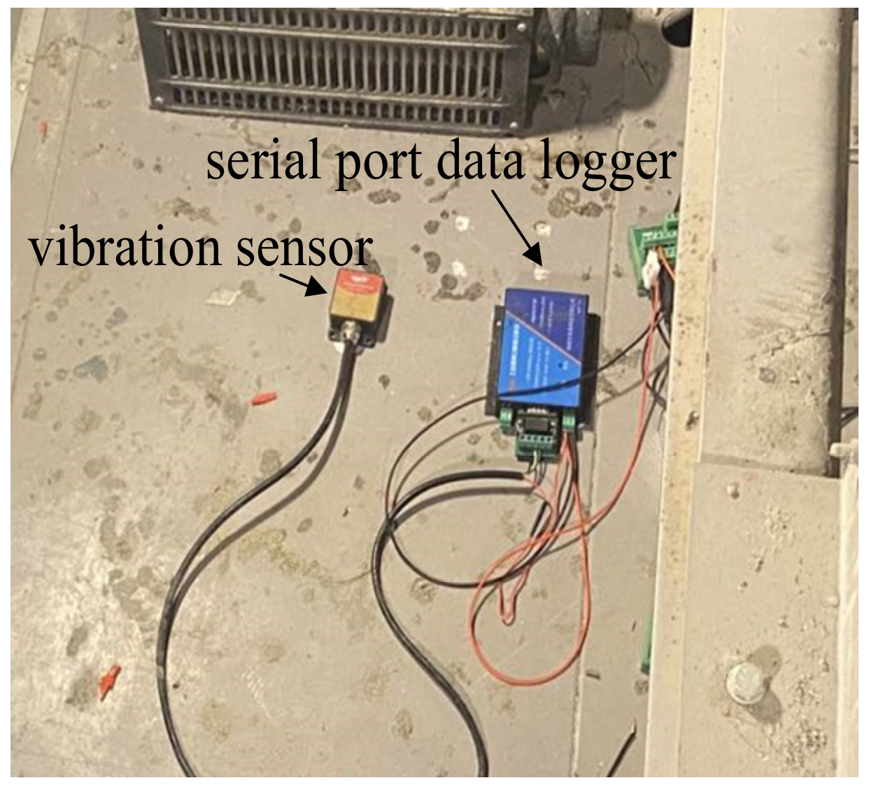
Figure 1 shows a signal acquisition device arranged on top of an elevator car, including the vibration sensor to record three-axis (X, Y, and Z) vibration data and a serial port data logger to record data. The vibration sensor is installed on the top of the elevator car through the serial port data logger to obtain the elevator car vibration signal and sample the vibration signal at a frequency of 200 Hz.

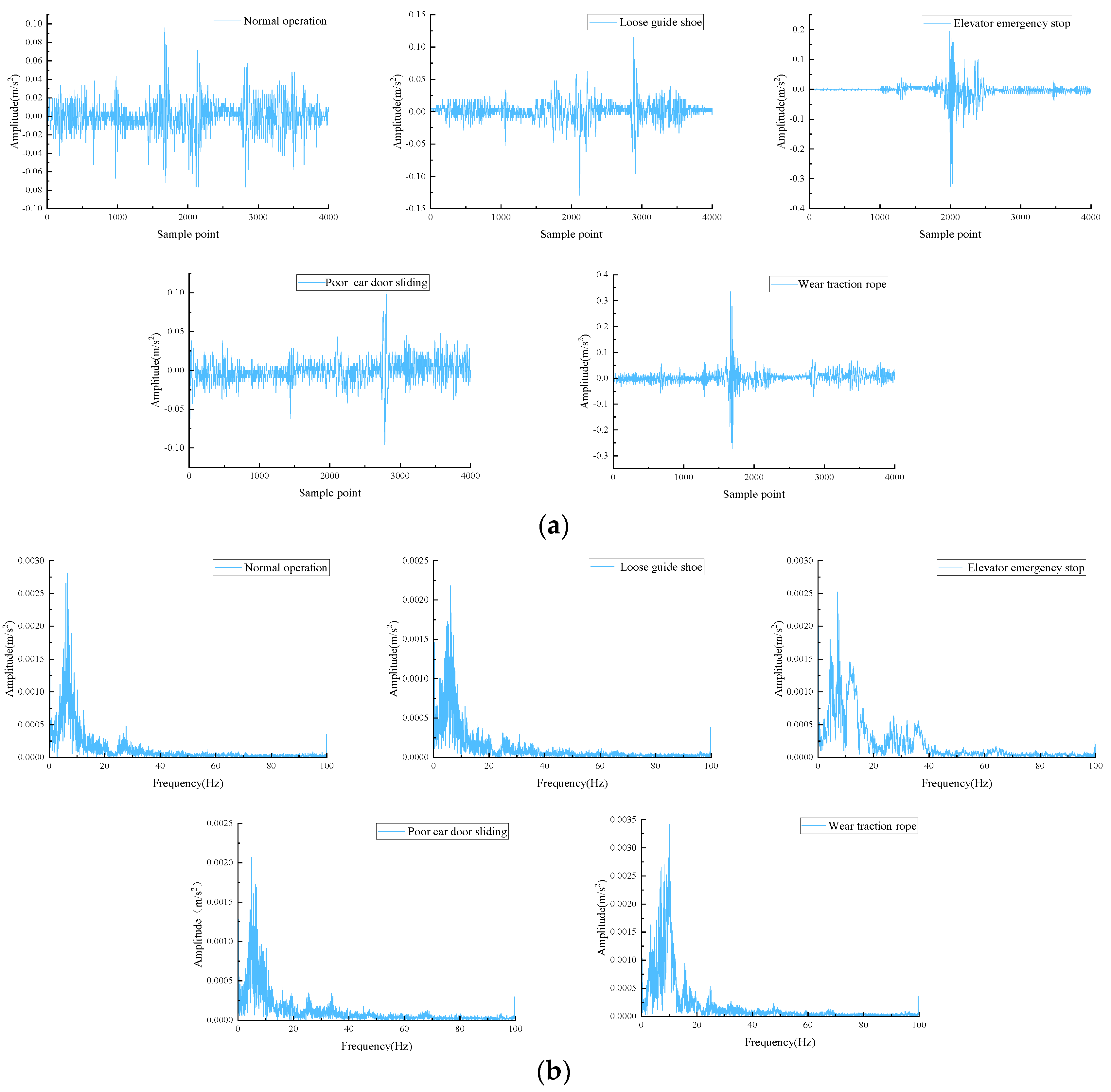
Elevator faults are typically manifested in the horizontal vibration signal. The horizontal vibration signal is divided into the X-axis and the Y-axis; after experiments, the Y-axis vibration signal is more accurate for elevator fault diagnosis, so the Y-axis vibration signal is used for elevator fault diagnosis. The dataset contains signals from five states: normal operation, loose guide shoe, elevator emergency stop, poor car door sliding, and wear traction rope. A total of 650 samples make up the original dataset, and the length of each set of signals is 4000.

The time domain and frequency domain waveforms of different conditions of vibration signal are shown in Figure 2. Figure 2a reveals that the normal signal is relatively stable in the time domain, whereas fault signals are larger amplitudes and irregular impacts. As seen in Figure 2b, the faulty conditions demonstrate irregular amplitudes between 0 and 40 Hz compared to normal operation. Observation of the time and frequency domain plots indicates that the elevator car vibration signal is nonstationary and nonperiodic in nature. Therefore, construction of a multi-dimensional feature vector is necessary in order to extract fault characteristics from the signals.

2.2. Elevator Vibration Signals

Elevator fault vibration signals cannot be fully represented by a single domain alone [14]; in extracting fault features in a single domain, it is difficult to include fault features fully and accurately. The multi-domain features reflect the operation state of the elevator, extracting the time domain, frequency domain, and entropy features of elevator vibration signals. Specifically, 11 time-domain, 12 frequency-domain, and 3 entropy features are extracted from the elevator car vibration signal, comprising a 26-dimensional multi-domain feature set.

Table 1. Multi-domain features.

Feature Type	Serial Number	Feature Name	Feature Type	Serial Number	Feature Name
Time domain characteristics	1	Average value	Frequency domain characteristics	15	Mean value of amplitude
	2	Standard deviation		16	Standard deviation of amplitude
	3	Square root amplitude		17	Amplitude skewness
	4	Root mean square		18	Crest factor
	5	Peak value		19	Frequency center of gravity
	6	Skewness
	7	Sharpness		20	Variance frequency
	8	Peaking factor		21	RMS frequency
	9	Margin factor		22	Mean square frequency
	10	Waveform factor
	11	Pulse index		23	Spectral form factor
Entropy feature	12	Approximate entropy		24	Spectral width factor
	13	Sample entropy		2	Spectral skewness
	14	Fuzzy entropy		26	Spectral crag

details the multi-domain features extracted.

3. Sample-Balancing Method Based on RFE-SMOTE-Tomek

In reality, the fault data samples of the elevator are much smaller than the normal data samples, and there is an imbalance of sample categories in the obtained dataset. This imbalance hinders effective model training and fault diagnosis. To address this problem, RFE-SMOTE-Tomek is proposed to oversample the samples. Redundant features can result in the generation of new samples that are not conducive to model training. RFE combined with random forests performs feature filtering on raw features to remove redundant features while reducing the dimensionality of the data. After feature optimization, the new samples generated are more meaningful and the quality of oversample is improved. The optimized features are oversampled by SMOTE-Tomek to obtain the sample balanced dataset. The flow is shown in Figure 3.

3.1. RFE-RF

Feature recursive elimination is performed through iterative model training [15]. All initial features were provided to random forest (RF) for ranking by importance. The least important features are removed; then, the retained features are re-fed into the model for the feature importance ranking, and the iterations are performed repeatedly to finally obtain the optimal set of features.

3.2. SMOTE-Tomek

3.2.1. SMOTE

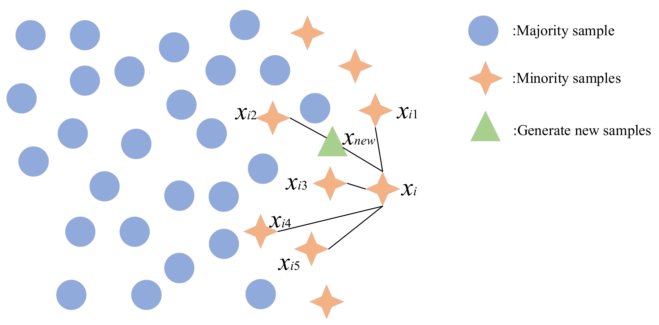
The SMOTE oversampling method is proposed by Chlawla to increase the minority class samples in the dataset by interpolating the minority class samples to generate new samples to achieve sample balance. The basic principle is shown in Figure 4.

SMOTE algorithm steps:

(1)

First, traverse the minority class samples and select each of them in turn (sample xi); compute the distance from xi to the other samples in terms of the Euclidean distance to obtain its k-nearest neighbor;

(2)

Randomly select some nearest neighbors to generate a new sample by linear interpolation with sample xi. The expression is as in Equation (1):

$$x_{new}=x_i+(x_i{}_j-x_i)\theta ,$$

(1)

where θ is a random number between (0, 1).

3.2.2. Tomek

Tomek Links is an undersampling method. Tomek Links sample pairs are pairs of connections between nearest neighbor samples of opposite classes [16]. The principle of the algorithm is as follows:

For any sample pair (x_i,x_j), compute the Euclidean distance d(x_i,x_j) between sample pair if there does not exist any sample x_k, such that d(x_k,x_i) < d(x_i,x_j) or d(x_k,x_j) < d(x_i,x_j) holds.

Then, the sample pair (x_i,x_j), located at the boundary of the class, is a Tomek Links sample pair. Therefore, the Tomek Links samples belonging to the newly generated samples are eliminated.

4. XGBoost Parameter Optimization Method Based on IAO Algorithm

The hyperparameters of XGBoost directly affect the classification effect, and different combinations of hyperparameters yield varying classification effects. In order to obtain the optimal combination of hyperparameters, the IAO algorithm is used to search for the hyperparameters. Compared with other group optimization algorithms, the AO algorithm has the advantages of powerful search ability, fast convergence speed, and high accuracy. However, when the problem is complex, the AO algorithm, prone to fall into local optimization, easily leads to the premature convergence of the algorithm. The AO algorithm is improved to address this problem.

4.1. AO Algorithm

The AO algorithm is developed and explored through four hunting strategies [17]. The iterative process of the AO algorithm optimization search consists of the following steps:

(1)

Expanded search (X₁)

The Aquila flies from a high altitude to determine the region of the search space. The expression is shown in Equation (2):

$$\begin{array}{c}{X}_1\left(t+1\right)=X_{best}\left(t\right)\times \left(1-\frac{t}{T}\right)+\left(X_M\left(t\right)-X_{best}\left(t\right)\right)*R\\ X_M\left(t\right)=\frac{1}{N}{\displaystyle {\displaystyle \sum }_{i=1}^N}{X}_i\left(t\right) ,{\forall }_j=1,2,\cdots ,dim\end{array}$$

(2)

where X₁(t + 1) is the solution of the next iteration; X_best(t) is the optimal solution obtained before the tth iteration; X_M(t) is the mean of the current population; R is the random number of (0, 1); t is the number of the current iteration; T is the maximum number of iterations; and dim is the dimension of the variable.

(2)

Narrowing the scope of exploration (X₂)

Aquila narrows the selected area, explores the target prey, and prepares to attack. The expression is as in Equation (3):

$$X_2\left(t+1\right)=X_{best}\left(t\right)\times Levy\left(D\right)+X_R\left(t\right)+\left(y-x\right)*R,$$

(3)

where D denotes the dimension space; X_R(t) is a random solution in the range [1,N]; and Levy(D) is the levy flight distribution function.

(3)

Expanded development (X₃)

The Aquila utilizes a selected target area to approach its prey and attack. The expression is as in Equation (4):

$$X_3\left(t+1\right)=\left(X_{best}\left(t\right)-X_M\left(t\right)\right)\times \alpha -R+\left(\left(UB-LB\right)\times rand+LB\right)\times \delta ,$$

(4)

where α and δ are adjustment parameters in (0, 1); LB is the upper bound of the problem; and the UB score is the lower bound of the problem.

(4)

Reducing the scope of development (X₄)

When the Aquila approaches the target, it moves randomly and attacks according to the position of the prey. The expression is as in Equation (5):

$$\begin{array}{c}{X}_4\left(t+1\right)=QF\times X_{best}\left(t\right)-(G_1\times \left(1-X\left(t\right)\right)-G_2\times Levy(D)+R\times G_1\\ QF\left(t\right)=t^{\frac{2\times R-1}{{(1-T)}^2}} \\ G_1=2\times R-1\\ G_2=2\times \left(1-\frac{t}{T}\right)\end{array}$$

(5)

where QF is the quality function used to balance the search strategy; G₁ denotes the different methods used by the Aquila to pursue the prey; and G₂ denotes the decreasing value from 2 to 0, representing the flight slope of the Aquila.

4.2. IAO Algorithm

The problem solved by the AO algorithm can easily fall into the local optimum when complex, with this tendency leading to the premature convergence of the algorithm. Tent chaotic mapping, nonlinear inertia weights, and nonlinear convergence factors are introduced to optimize the AO algorithm in terms of balancing the ability of the global search and the local search and enhancing the ability of jumping out of the local optimum and the global search.

4.2.1. Tent Chaotic

The adoption of a uniform distribution for the initial population enables the optimization algorithm to efficiently approximate the global optimal solution. In the AO algorithm, the position of the initial population is randomly generated and may be unevenly distributed. Tent chaotic mapping is introduced to generate a more evenly distributed initial population. The expression is shown in Equation (6):

$$x_{i+1}=\left\{\begin{array}{l}2x_{i,}{x}_i<0.5\\ 2(1-x_i),x_i\ge 0.5\end{array}\right..$$

(6)

4.2.2. Nonlinear Inertia Weights

Nonlinear inertia weights balance the ability of the global and local search. In the early stage of the algorithm iteration, the inertia weights should be larger, and the Aquila goes to the neighborhood of the target value faster with better global search capability. In addition, in the later stage of the algorithm iteration, the inertia weights should be smaller, making the Aquila explore at a lower speed to avoid falling into the local optimum, while attaining better local search ability. The expression for the nonlinear inertia weights is as follows:

$$\omega =\cos {(\frac{0.5\pi t}{T})}^n.$$

(7)

where T is the maximum number of iterations; n is the inertia weight control parameter; and the larger n tends towards local search development.

The improved expression is as follows:

$$X_1\left(t+1\right)=X_{best}\left(t\right)\times \left(1-\cos {(\frac{0.5\pi t}{T})}^n\right)+\left(X_M\left(t\right)-X_{best}\left(t\right)\right)*R.$$

(8)

4.2.3. Nonlinear Convergence Factor

In the Aquila optimization algorithm, in the reduced exploitation range, G₂ is the flight slope of the Aquila, and the value is a linearly decreasing convergence factor from 2 to 0. This may result in the Aquila not being able to move efficiently to the prey position. Introducing a nonlinear convergence factor can make the algorithm converge to the optimal solution faster while avoiding falling into a local optimum.

$$G_2=\frac{2}{1+e^{Q(2\frac{t}{T}-1)}},$$

(9)

where Q = 9.903438.

4.3. XGBoost Model

The XGBoost model is an implementation of the gradient boosting tree algorithm, which is used to construct a model by combining multiple decision trees. In this way, models can be constructed with higher accuracy. XGBoost model performance is improved by iteratively training a series of decision trees. Each new decision tree is trained on the residuals of the previous decision trees to reduce the error of the model on the training data. XGBoost model:

$${\stackrel{⌢}{y}}_i={\displaystyle \sum _{k=1}^K{f}_k(x_i)},f_k\in F$$

(10)

$$F=\left\{\left.f(x)={\omega }_{q(x)}\right\}\right.,q:R^m\to T,\omega \in R^T,$$

(11)

where (x_i,y_i) is the dataset; xi is the feature vector of the ith sample; y_i is the label of the ith sample; f_k corresponds to an independent tree model; F is the set of all trees; q is the mapping of the feature vectors to the corresponding leaf nodes; and ω_q(x) denotes the leaf weights. The objective function of the model is as follows:

$$O={\displaystyle \sum _{i=1}^{n}l(y_i,{\stackrel{⌢}{y}}_i)}+{\displaystyle \sum _{k=1}^K\Omega (f_k)}$$

(12)

$$\Omega (f)=\gamma T+\frac{1}{2}\lambda {\omega }^2,$$

(13)

where ${\displaystyle \sum _{i=1}^{n}l(y_i,{\stackrel{⌢}{y}}_i)}$ is the training loss function; ${\stackrel{⌢}{y}}_i$ is the predicted value; $y_i$ is the test value; ${\displaystyle \sum _{k=1}^K\Omega (f_k)}$ is the penalty function; and $\gamma$ and $\lambda$ are the regularization parameters.

4.4. IAO-XGBoost Hyperparameter Optimization Process

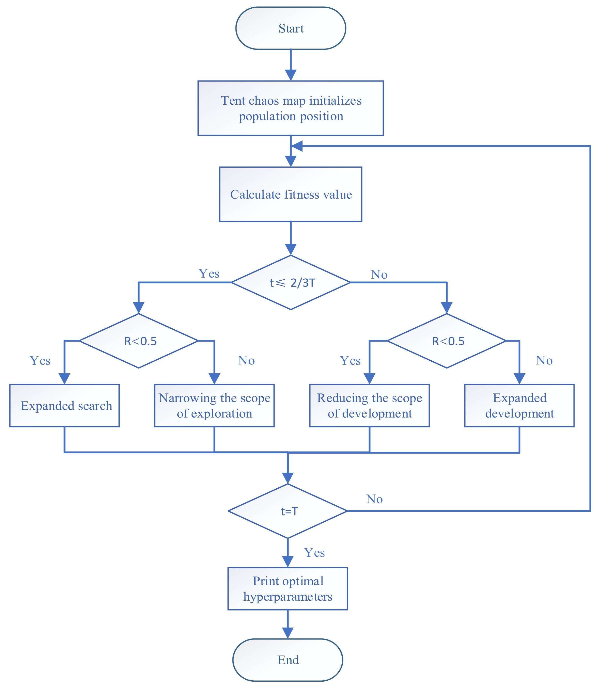
The IAO-XGBoost algorithm flow is as follows, and the flow chart is shown in Figure 5.

(1)

Generating initial population through Tent chaotic mapping;

(2)

The error rate of the XGBoost model is used as a fitness function to calculate the fitness value;

(3)

Using the improved strategy to find the optimal hyperparameter combination;

(4)

Determining whether the iteration termination conditions are met; if so, the algorithm outputs the optimal hyperparameter combination; otherwise, it returns to step (2).

5. Elevator Car Fault Diagnosis Example Analysis

5.1. Experimental Data

In this study, 650 sets of data are collected from the vibration sensor at the top of the elevator car, with a ratio of 7:3 between the training set and the test set. The dataset includes five states: normal operation, loose guide shoe, elevator emergency stop, poor car door sliding, and wear traction rope. The distribution of the training and test set samples is shown in

Table 2. The case of different types of sample data.

Data Type	Training Set	Test Set	Amount
Normal operation	217	94	311
Loose guide shoe	120	51	171
Elevator emergency stop	41	18	59
Poor car door sliding	39	17	56
Wear of traction rope	37	16	53
Amount	455	195	650

.

5.2. Analysis of the Results of Sample Balancing Based on RFE-SMOTE-Tomek

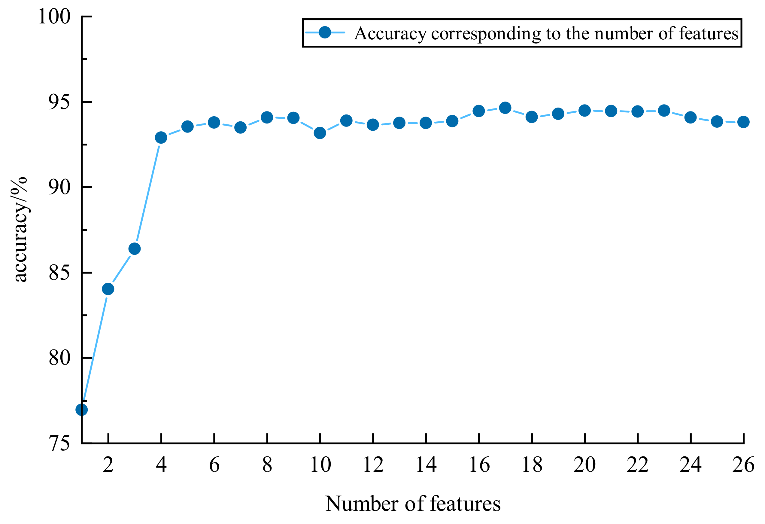
The number of features affect both sample balancing and the fault diagnosis results. In order to select the optimal feature set, different sets of features are inputted into the XGBoost model, and the corresponding fault diagnosis accuracies are obtained. The initial hyperparameters of the XGBoost model are preset as n_estimators = 100; max_depth = 4, learning rate = 0.1; subsample = 1; colsample_bytree = 1. The results of the effect of different numbers of features on fault accuracy are shown in Figure 6.

Reducing the dimensionality of the data by removing redundant features helps mitigate the impact of such features on the accuracy of fault diagnosis. However, eliminating too many features may lead to the removal of useful ones. It is essential to determine the optimal number of features. From Figure 5, when the number of features is 17, the accuracy of fault diagnosis reaches its maximum, which is 94.63%. According to the effect of different numbers of features on fault diagnosis, the top 17 features, in terms of importance ranking, are selected as the preferred feature dataset.

To validate the effectiveness of the RFE-SMOTE-Tomek sample-balancing method, the original feature dataset, the dataset after feature optimization, and the dataset processed by different sample-balancing methods (SMOTE, Borderline-SMOTE, SMOTE-ENN, SMOTE-Tomek, and SMOTE-Tomek) are selected for comparison. The fault diagnosis model is XGBoost. The sample distribution of the training set before and after sample balancing via RFE-SMOTE-Tomek is shown in

Table 3. The distribution of the number of samples before and after the training set sample balance.

Data Type	Original Dataset	Sample Balanced Dataset
Normal	217	217
Loose guide shoe	120	217
Elevator emergency stop	41	215
Poor sliding of car door	39	169
Wear of traction rope	37	160

. The comparison of fault diagnosis accuracy under different sample processing methods is shown in

Table 4. Comparison of fault diagnosis accuracy under different sample processing methods.

Sample Processing Methods	Accuracy/%
Original dataset	93.81
RFE Feature Selection	94.63
SMOTE	95.50
Borderline-SMOTE	96.78
SMOTE-ENN	96.75
SMOTE-Tomek	97.47
RFE-SMOTE-Tomek	97.88

.

Table 4 show that the accuracy of fault diagnosis is 3.54–4.36% higher for the dataset with the sample-balancing process compared to the dataset without the sample-balancing process. Compared to the sample-balancing methods of SMOTE, Borderline-SMOTE, SMOTE-ENN, and SMOTE-Tomek, the proposed RFE-SMOTE-Tomek sample-balancing method in this study improves the accuracy of fault diagnosis by 2.38%, 1.1%, 1.13%, and 0.41%, respectively. From the results, the accuracy of fault diagnosis is improved by the sample-balancing method proposed in this study. Reducing the feature dimension by eliminating invalid features through the RFE method and reducing the impact of redundant features when sampling via SMOTE-Tomek enable the model to better learn a small number of classes of samples and improve its fault diagnosis ability.

5.3. Analysis of Results of XGBoost Parameter Optimization Method Based on IAO Algorithm

5.3.1. IAO Algorithm Performance Testing

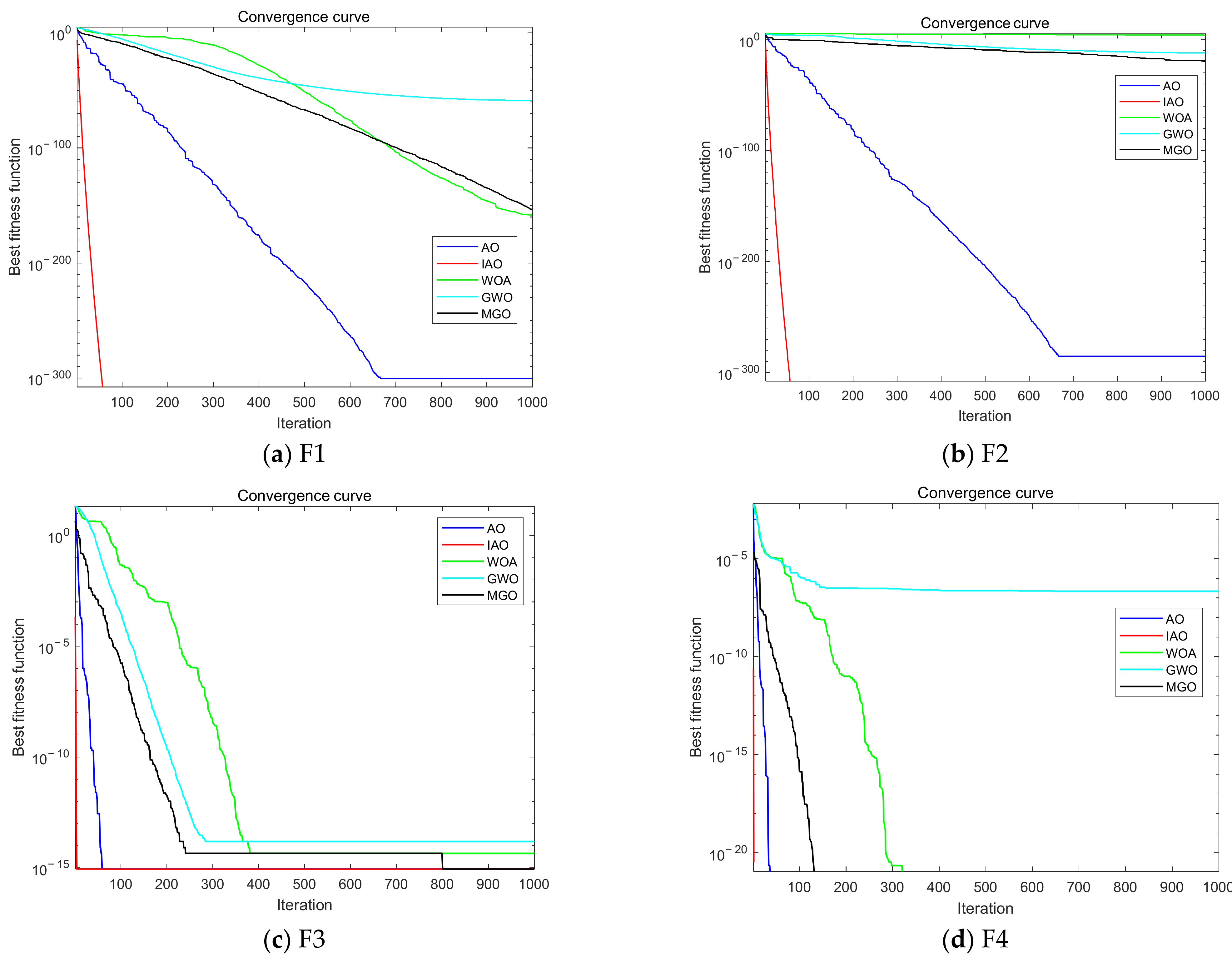
To verify the superiority of the IAO algorithm over other algorithms, a comparative experiment is conducted between the IAO algorithm and the AO algorithm, whale optimization algorithm (WOA), gray wolf optimization (GWO) algorithm, and mountain gazelle optimization (MGO) algorithm. The maximum number of iterations of the experimental parameters is 1000, and the population size is 20. The algorithm’s performance test functions are presented in

Table 5. Algorithm performance test function.

Function	Formulas	Dimension	Realm	Optimum Value
F1	$f_1(x)={\displaystyle \sum _{i=1}^n{x}_i^2}$	30	[−100, 100]	0
F2	$f_2(x)={{\displaystyle \sum _{i=1}^n({\displaystyle \sum _{j-1}^{i=1}{x}_j})}}^2$	30	[−100, 100]	0
F3	$f_3(x)=-20\exp (-0.2\sqrt{\frac{1}{n}{\displaystyle \sum _{i=1}^n{x}_i^2}})-\exp (\frac{1}{n}{\displaystyle \sum _{i=1}^n\cos (2\pi x_i)})$	30	[−32, 32]	0
F4	$f_4(x)=\frac{1}{4000}{\displaystyle \sum _{i=1}^n{x}_i^2-{\displaystyle \prod _{i=1}^n\cos (\frac{x_i}{\sqrt{i}})}+1}$	30	[−600, 600]	0

, which includes single-peak functions (F1 and F2) and multi-peak functions (F3 and F4).

Single-peak functions have no extreme points and only a unique optimal solution, while multi-peak functions have multiple extreme points and an optimal solution. The former verify the convergence speed and the ability of the algorithm to find the optimum, while the latter verify the ability of the algorithm to jump out of the local optimum.

Figure 7 shows the convergence curves of each algorithm under different algorithm test functions. From the analysis of convergence speed, it can be seen from Figure 7a,b that WOA, GWO, and MGO did not find the extreme point during 1000 iterations. Due to the introduction of Tent chaotic mapping by IAO, the global optimal value can be found faster than the AO algorithm. The IAO algorithm has fallen into local optima, while the IAO algorithm, which introduces nonlinear inertia weights and nonlinear convergence factor strategies, overcomes the problem of falling into local optima. The IAO algorithm has found the extreme point 0 near 50 iterations. The other four algorithms of the IAO algorithm significantly improve the global search ability and convergence speed, moving towards the global optimal search and avoiding local optimal values.

Figure 7c shows that the WOA and GWO algorithms have fallen into local optima, while AO, IAO, and MGO have found global optima. The IAO algorithm converges faster than the AO algorithm, and MGO jumps out of local optima and finds global optima after 800 iterations. The introduction of strategy in the IAO algorithm improves convergence efficiency and the ability to jump out of local optima compared to the AO and MGO algorithms.

Figure 7d shows that the AO, IAO, WOA, and GWO algorithms have found global optima, while the GWO algorithm has fallen into local optima. WOA repeatedly falls into local optima and jumps out of local optima, ultimately finding the global optimum. The IAO algorithm quickly converges and finds the global optimal point.

In summary, the IAO algorithm avoids falling into local optima and has a faster convergence speed than other algorithms. It can quickly find the global optimal value, indicating that the introduced strategy can effectively improve the algorithm’s performance.

5.3.2. Analysis of Fault Diagnosis Results Based on IAO-XGBoost

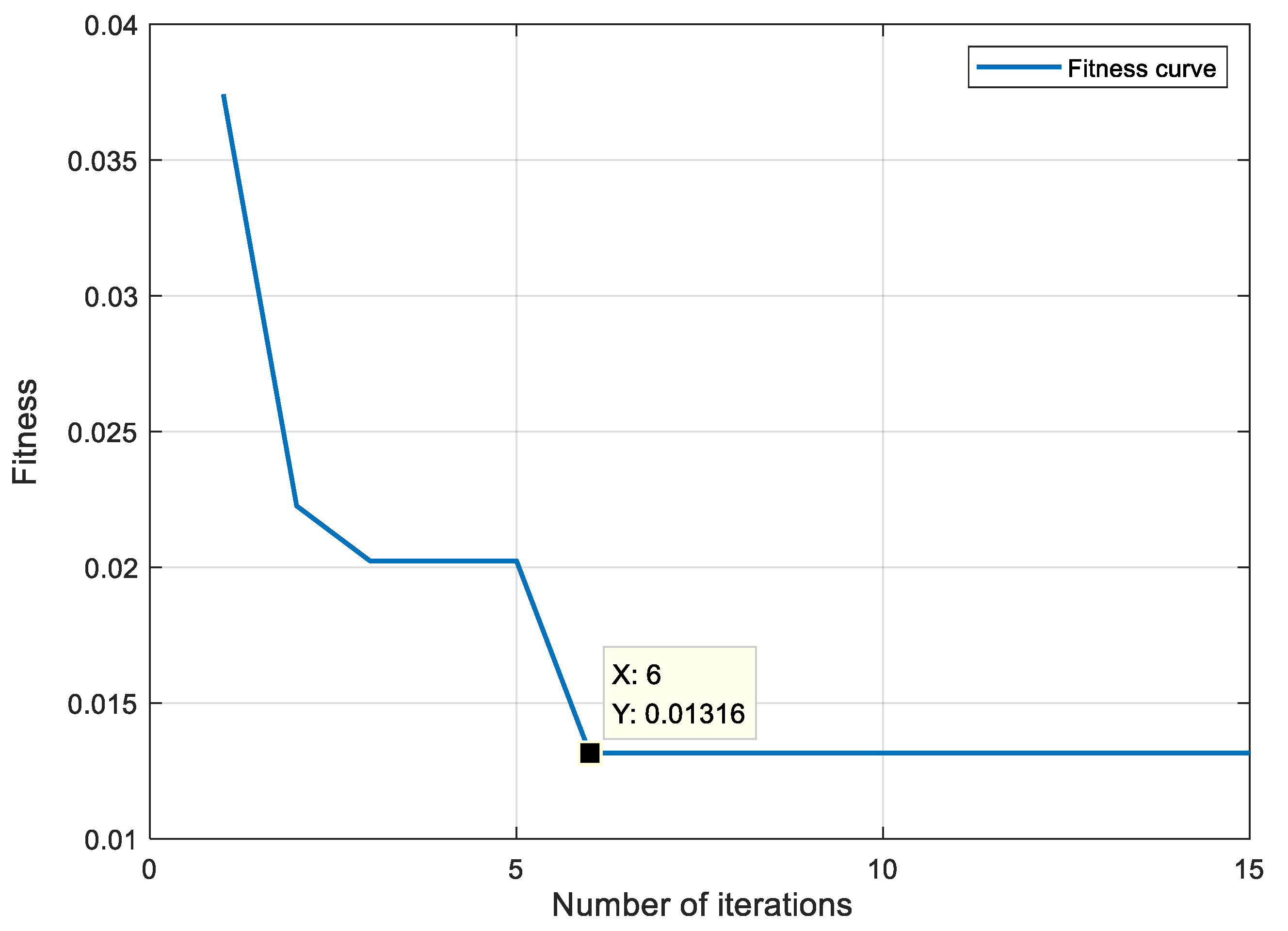
XGBoost model hyperparameters have a significant effect on the effectiveness of the model in classification training. During training, the max_depth parameter determines the depth of the decision trees in the model. Setting it too high allows the model to learn more features but increases the risk of overfitting and complexity; conversely, a max_depth that is too low results in a simplistic model that fails to capture the full features of the data, leading to underfitting. Additionally, n_estimators, learning_rate, subsample, and colsample_bytree collectively influence the model’s learning performance and classification ability. The IAO algorithm is utilized for iterative optimization of the above five hyperparameters. The number of populations is 20, the maximum number of iterations is 15, and the fitness function is the error rate of the model. The adaptation degree change curve is shown in Figure 8.

The fitness change curve shows that when the iteration reaches six times, the fitness value is 0.01316 and the algorithm converges. The optimal hyperparameter combination is obtained, and the parameters are shown in

Table 6. Optimized parameters.

Parameter Name	Optimum Value
n_estimators	47
max_depth	11
learning rate	0.28
subsample	1
colsample_bytree	0.76

.

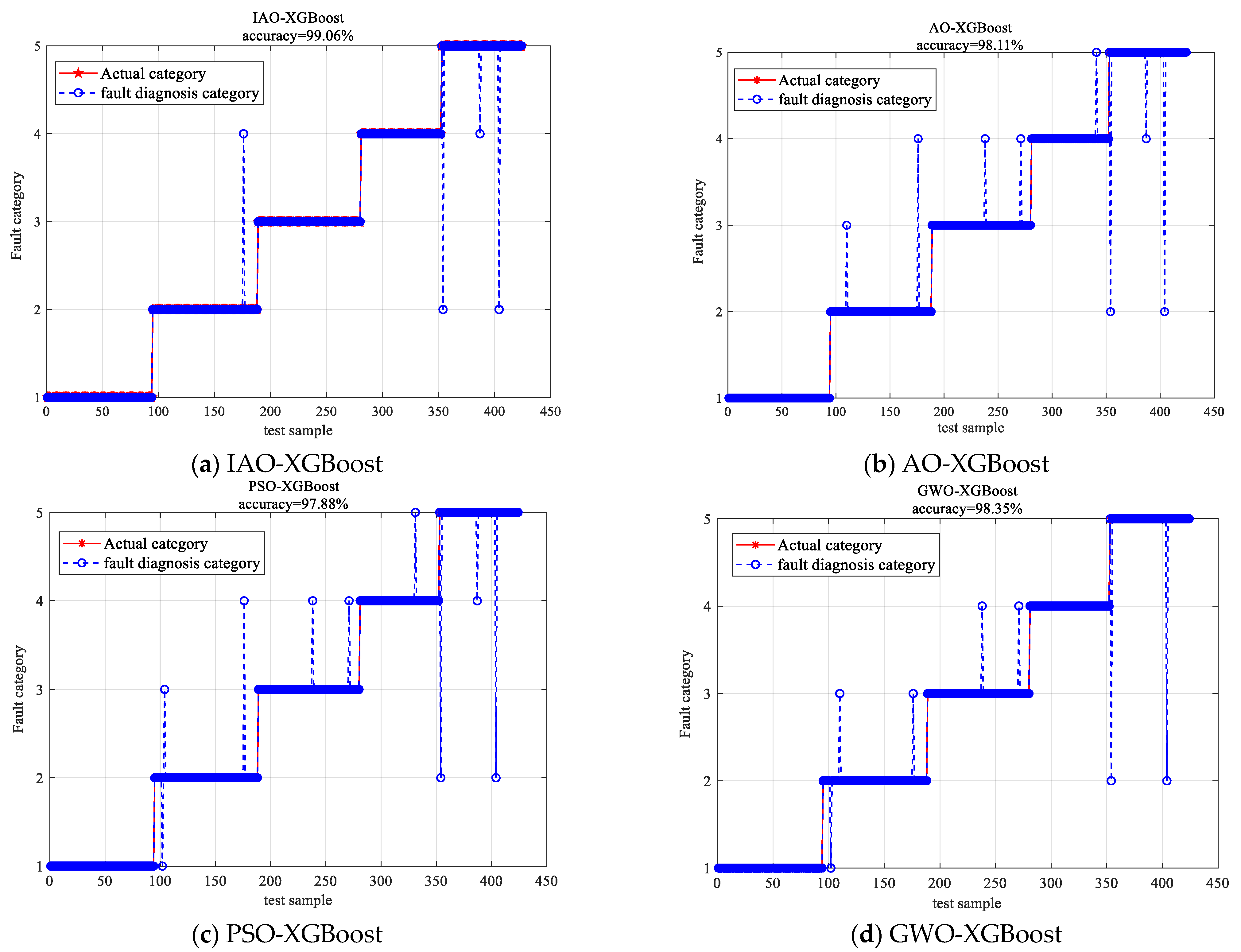
To validate the effectiveness of the IAO-XGBoost model in elevator car fault diagnosis, experiments are conducted using AO-XGBoost, PSO-XGBoost, GWO-XGBoost, and IAO-XGBoost on the same training and test sets. The results of the fault diagnosis are presented in Figure 9.

From Figure 9, the fault diagnosis accuracy of the IAO-XGBoost model reaches 99.06%. The fault diagnosis accuracies of AO-XGBoost, PSO-XGBoost, and GWO-XGBoost are 98.11%, 97.88%, and 98.35%, respectively. The results show that the AO algorithm, which incorporates Tent chaotic mapping, nonlinear inertia weights, and nonlinear convergence factor strategies, has superior optimization-seeking ability compared to the other algorithms. The proposed IAO-XGBoost model demonstrates better classification ability than the other three models, highlighting its higher reliability and superiority for elevator car fault diagnosis.

To further illustrate the reliability and accuracy of the IAO-XGBoost model, the IAO-XGBoost model is compared with XGBoost, LightGBM, and RF, and the fault diagnosis results are shown in

Table 7. Diagnosis results of different fault diagnosis models.

Fault Diagnosis Model	Accuracy/%	Kappa Factor	Time/s
RF	96.69	0.958	0.6673
LightGBM	96.93	0.961	0.1374
XGBoost	97.88	0.973	0.0522
IAO-XGBoost	99.06	0.988	0.0442

.

As shown in Table 6, the fault diagnosis accuracy of the IAO-XGBoost model proposed in this study can reach 99.06%, which improves by 2.37%, 2.13%, and 1.18% compared to RF, LightGBM, and XGBoost models, respectively. Moreover, it has a significant advantage in diagnosis time. Compared to RF, LightGMB, and XGBoost models, the training time has been saved by 93.3%, 69.2%, and 15.3%, respectively. The reduction of training time can help reduce the performance requirements for computer hardware. The kappa coefficient, combined with accuracy and recall, can comprehensively evaluate the diagnostic performance of the model. The higher the kappa coefficient, the more consistent the judgment of fault diagnosis results and the better the model stability. The IAO-XGBoost model proposed in this article is used for fault diagnosis, and the Kappa coefficient is the highest among the five methods, reaching 0.988, and indicating that the proposed model has a more reliable fault diagnosis effect.

6. Conclusions

In the IAO-XGBoost-based elevator fault diagnosis method under unbalanced samples proposed in this study, the IAO algorithm improves the ability of the algorithm to jump out of the local optimum compared with the traditional swarm intelligence algorithm. The model optimized by the algorithm has a better combination of hyperparameters, improving the accuracy and reliability of the model. At the same time, taking into account the fact that the elevator fault samples are small and the sample categories are unbalanced, the classification performance of fault diagnosis is improved. Combined with the example analysis, the conclusions obtained are as follows:

• The method of RFE-SMOTE-Tomek reduces the influence of redundant features on the generation of new samples by SMOTE-Tomek, obtains better sample balanced data, and improves the ability of subsequent fault diagnosis;
• The AO algorithm is improved by introducing Tent chaotic mapping, nonlinear inertia weights, and nonlinear convergence factors, which can effectively improve the convergence speed and optimization- seeking performance of the algorithm;
• With the proposed method of sample balancing, RFE-SMOTE-Tomek, combined with the elevator fault diagnosis model of IAO-XGBoost, which accurately identifies the state of the elevator, fault diagnosis accuracy can reach 99.06%.

The method proposed in this article has achieved good results with respect to sample imbalance in elevators. Although this article mainly focuses on elevator fault diagnosis, the proposed method can be extended to the long-term operational health monitoring of elevators in the future. Through real-time monitoring and diagnosis, potential faults can be better predicted, and preventive maintenance measures can be taken, thereby extending the service life of elevators and improving their reliability.

References

- Pan, W.; Gong, W.L.; Liu, Z.H. Study on risk control and management model for special equipment. J. Saf. Environ. 2023, 1–10. [Google Scholar] [CrossRef]
- Zheng, Q. Elevator Fault Diagnosis and Prediction Based on Data Feature Mining and Machine Learning. Master’s Thesis, Zhejiang University, Hangzhou, China, 2022. [Google Scholar] [CrossRef]
- Jiang, Z.; Zhao, L.; Lu, Y. A semi-supervised resampling method for class-imbalanced learning. Expert Syst. Appl. 2023, 221, 119733. [Google Scholar] [CrossRef]
- Liu, X.B. Intelligent Fault Diagnosis of Wind Turbine Drivetrain based on Deep Learning. Ph.D. Thesis, North China Electric Power University, Beijing, China, 2022. [Google Scholar] [CrossRef]
- Shao, Y.W.; Cheng, J.Y.; Ling, C.Y. Gearbox fault diagnosis with small training samples: An improved deep forest based method. Acta Aeronaut. Astronaut. Sin. 2022, 43, 118–132. [Google Scholar] [CrossRef]
- Li, A.; Han, M.; Mu, D.L. Survey of multi-class imbalanced data classification methods. Appl. Res. Comput. 2022, 39, 3534–3545. [Google Scholar] [CrossRef]
- Chawla, N.V.; Bowyer, K.W.; Hall, L.O. SMOTE: Synthetic minority over-sampling technique. J. Artif. Intell. Res. 2002, 16, 321–357. [Google Scholar] [CrossRef]
- Yuan, X.; Yuan, Z.; Wei, K. A multi-fault diagnosis method based on improved SMOTE for class-imbalanced data. Can. J. Chem. Eng. 2023, 101, 1986–2001. [Google Scholar] [CrossRef]
- Liu, Y.P.; He, J.H.; Xu, Z.Q. Equalization Method of Power Transformer Fault Sample Based on SVM SMOTE. High Volt. Eng. 2020, 46, 2522–2529. [Google Scholar] [CrossRef]
- Duan, F.; Zhang, S.; Yuan, Y. An oversampling method of unbalanced data for mechanical fault diagnosis based on MeanRadius-SMOTE. Sensors 2022, 22, 5166. [Google Scholar] [CrossRef] [PubMed]
- Zhu, L.; Wang, X.H.; Li, H. Transformer Fault Diagnosis Method Based on Variant Sparrow Search Algorithm and lmproved SMOTE Undet Unbalanced Samples. High Volt. Eng. 2023, 1–9. [Google Scholar] [CrossRef]
- Zhang, D.; Qian, L.; Mao, B. A data-driven design for fault detection of wind turbines using random forests and XGboost. IEEE Access 2018, 6, 21020–21031. [Google Scholar] [CrossRef]
- Zhang, Y.W.; Feng, B. Fault diagnosis method for oil-immersed transformer based on XGBoost optimized by genetic algorithm. Electr. Power Autom. Equip. 2021, 41, 200–206. [Google Scholar] [CrossRef]
- Fu, S.; Zhong, S.S.; Ling, L. Gas turbine fault diagnosis method under small sample based on transfer learning. Comput. Integr. Manuf. Syst. 2021, 27, 3450–3461. [Google Scholar] [CrossRef]
- He, H.Y.; Huang, G.Y.; Zhang, B. lntrusion Detection Model Based on Extra Trees-recursive Feature Elimination and LightGBM. Netinfo Secur. 2022, 22, 64–71. [Google Scholar] [CrossRef]
- Zhao, K.L.; Jin, X.L.; Wang, Y.Z. Survey on Few-shot Learning. J. Softw. 2021, 32, 349–369. [Google Scholar] [CrossRef]
- Abualigah, H.Y.; Yousri, D.; Abd, E.M. Aquila optimizer: A novel meta-heuristic optimization algorithm. Comput. Ind. Eng. 2021, 157, 107250. [Google Scholar] [CrossRef]