Vehicle State and Road Adhesion Coefficient Joint Estimation Based on High-Order Cubature Kalman Algorithm

Abstract

With regard to the rear-drive in-wheel motor vehicle, this paper studies the joint estimation method for the vehicle state and road adhesion coefficient. A nonlinear seven degrees of freedom vehicle estimation model and a tire estimation model are established. A vehicle driving state estimator and a road adhesion coefficient estimator based on the generalized high-order cubature Kalman filter (GHCKF) algorithm are designed. The vehicle state estimator combines the vehicle model and the tire model to calculate the vehicle state parameters, provides the state parameters for the road adhesion coefficient estimator, and realizes the real-time estimation of the road adhesion coefficient. The exponential fading memory adaptive algorithm is used to update the measurement noise variance, and we upgrade the GHCKF to the adaptive generalized high-order cubature Kalman filter (AGHCKF), which estimates the vehicle state and road adhesion coefficient. The typical working conditions using the double GHCKF/AGHCKF estimation algorithm were simulated and analyzed. Then, high-and low-speed driving experiments based on typical working conditions were carried out. An integrated navigation system (INS), global positioning system (GPS), and real-time kinematic positioning (RTK) were used to collect the real-time data of the vehicle, and compare them with the estimated values of the joint estimator, to verify the feasibility of the vehicle-state–road-adhesion-coefficient joint estimator. We compared a high-order GHCKF algorithm, high-order improved AGHCKF algorithm, and a cubature Kalman filter (CKF) algorithm, and the simulation and experimental results show that the joint estimator using the CKF, GHCKF, and AGHCKF algorithms can realize the real-time estimation of the vehicle state and the road adhesion coefficient. The AGHCKF algorithm shows the best effectiveness and robustness of the three algorithms.

1. Introduction

With the rapid development of electric vehicle technology, the in-wheel motor, as a distributed drive component, is more and more widely used. The real-time and accurate acquisition of the vehicle driving state and road adhesion coefficient is also an urgent requirement for achieving active safety control. Due to the high cost of GPS, INS, and road-imaging technology, they are impossible to popularize in the automobile control process within a short time. Therefore, the real-time and accurate estimation of the vehicle driving state and road adhesion information based on distributed drive theory, combined with low-cost sensors, has become a research hotspot concerning the active safety control of in-wheel motor vehicles [1,2,3].

The Kalman filter algorithm has the advantage of recursive iteration, which can effectively suppress noise and improve the system accuracy. An extended Kalman filter (EKF) and unscented Kalman filter (UKF) are developed based on the classical Kalman filter algorithm. The Kalman filter method is widely used in the field of vehicle state estimation and road adhesion coefficient estimation [4,5,6]. Li et al. proposed a double radial basis function and extended Kalman filter (DRBF-EKF) method, which can adaptively adjust the network structure [7]. The radial basis function (RBF) neural network structure is improved via a k-means algorithm, and the EKF is used for noise filtering to improve the estimation accuracy, so as to realize the dynamic joint estimation of the vehicle sideslip angle and road adhesion coefficient. Huang et al. combined the EKF with the limited memory filter to improve the stability and anti-interference properties of the filter, which can effectively estimate the road adhesion coefficient [8]. Jin et al. proposed the method of a parallel UKF. A UKF that can adapt to a strong nonlinear system was used to estimate the vehicle inertia parameters, and a state-parameter joint observation system based on a vehicular parallel double UKF was designed, so that the vehicle still showed a high observation accuracy under heavy-load loading conditions [9]. In order to effectively solve the nonlinear problem in vehicle dynamics, a double unscented Kalman filter (DUKF) was run in parallel, to estimate the vehicle state and other parameters at the same time, and this achieved good results [10].

The EKF truncates the Taylor expansion of a nonlinear function by first-order linearization, ignoring other higher-order terms, and thereby transforming the nonlinear problem into a linear problem. The EKF algorithm may cause filtering divergence when the neglected high-order terms in the Taylor expansion result in significant errors; in addition, because the Jacobian matrix is required in the linearization process of the EKF, the cumbersome calculation process makes the method relatively difficult to implement. The UKF is an algorithm based on the combination of unscented transformation and Kalman filtering. This algorithm mainly uses the idea of the Kalman filter, but when subsequently solving the predicted value and measured value of the target, it needs to apply the sampling point for the calculation. The UKF approximates the n-dimensional target sampling points by designing weighted points, calculates the propagation of these weighted points through the nonlinear function, and obtains the updated filtering value through the nonlinear state equation, to conduct target tracking. The UKF effectively overcomes the EKF’s shortcomings of a low estimation accuracy and poor stability. However, it is difficult to ensure the positive definiteness of the state estimation covariance matrix in the calculation process of the UKF, and it is necessary to select a suitable set of parameters in order to obtain the ideal estimation results.

The cubature Kalman filter (CKF) is a new nonlinear Gaussian filtering method proposed by Canadian scholars in 2009 [11,12], which has been widely used in the field of vehicle control [13,14,15,16]. Qi presented a robust hierarchical estimation scheme for the vehicle driving state based on the maximum correntropy square-root cubature Kalman filter (MCSCKF), and achieved good results [17]. A longitudinal–lateral cooperative estimation algorithm based on an adaptive square-root cubature Kalman-filter (ASRCKF) was proposed by Chen, this algorithm can accurately estimate the vehicle status under different driving conditions [18].

The CKF relies on the determined cubature point to calculate the posterior probability density function. Compared with the EKF, it does not need to calculate the complex Jacobian matrix, and the filtering is more accurate and avoids the truncation error. Compared with the UKF, the cubature points of the CKF appear symmetrically in a lower one-dimensional subspace, and the weights of each cubature point are equal. It is not necessary to set the parameters in advance like the UKF. The selection method is simpler, the adaptability is stronger, and the calculation speed is faster. However, the filtering accuracy of CKF can only reach the third order, and its positive cubature point weight will cause the estimation point to cross the boundary or produce a complex form of estimation point, and when n is large enough, the cubature point may exceed the integral region [19]. Therefore, many scholars have deduced the high-order spherical-radial cubature rule based on the third-order spherical-radial cubature rule, proposed the high-order cubature Kalman filter (HCKF) and applied it [20,21,22]. HCKF needs to increase the order of both the volume criterion and the Gaussian Laguerre criterion when expanding the spherical radial integration to higher order, and calculate the area fraction of the n-dimensional hypersphere. The calculation process is complex, resulting in poor high-order scalability of the CKF algorithm. In order to overcome the above problems, GHCKF has been proposed and applied by relevant scholars. GHCKF applies the theory of numerical integration, which is simple in form, efficient in calculation and better in scalability [23,24,25].

In this paper, we will establish a state equation based on the seven degrees of freedom and the tire model of this vehicle. At the same time, we will establish a measurement equation based on measurement sensor data; in this way, a new research framework for vehicle state estimation and road adhesion coefficient estimation will be constructed. We propose a GHCKF estimator, which can estimate the vehicle state and road adhesion coefficient, respectively, and use the adaptive theory to upgrade the GHCKF to an AGHCKF estimator with a stronger robustness and effectiveness. In this paper, the CKF, GHCKF, and AGHCKF algorithms will be developed, and will also be compared through simulation and experiments to verify the superiority of the AGHCKF algorithm. A high-order Kalman estimator will provide a new and reliable method for vehicle state estimation and road adhesion coefficient estimation. As shown in Figure 1, state equations and measurement equations will be established, and Kalman and adaptive theory will be applied to build a CKF/GHCKF/AGHCKF algorithm, which will jointly estimate the vehicle state and road adhesion coefficient. The vehicle sensor measures the steering wheel angle, wheel speed, yaw rate, lateral/longitudinal acceleration, and other parameters, then inputs them into the seven degrees of freedom nonlinear vehicle model, the vehicle state estimator, and the road adhesion coefficient estimator. The vehicle model uses the measurement parameters to calculate the tire longitudinal force and lateral force, and the calculated values are provided to the vehicle state estimator, and then the longitudinal/lateral velocity and yaw rate are estimated via the vehicle state estimator. The vehicle state estimator feeds the estimated values back to the nonlinear vehicle model, calculating parameters such as the sideslip angle and the tire slip rate. The sideslip angle and the tire slip rate are sent to the Dugoff tire model for the calculation of the normalized tire longitudinal force and lateral force. The road adhesion coefficient estimator estimates the road adhesion coefficient via the measuring parameters and the normalizing tire force, and the results are fed back to the nonlinear vehicle model for the provision of reliable parameters for vehicle control.

This paper aims to design a new technical route for estimating vehicle status and road adhesion coefficient, develop a generalized high-order Kalman estimator based on adaptive theory, verify its progressiveness and robustness, and explore its application value. Firstly, establish a nonlinear dynamic vehicle model and tire model, and then design a vehicle state estimator and road adhesion coefficient estimator based on high-order Kalman filters. Then, upgrade the high-order Kalman algorithm combined with adaptive theory to an AGHCKF algorithm, build a simulation platform, design experimental plans, and finally verify the superiority of the AGHCKF algorithm by comparing and analyzing the simulation and experimental results, provide theoretical support for the application of this algorithm in vehicle testing.

2. Nonlinear Dynamic Vehicle Model

In this paper, a seven degrees of freedom nonlinear vehicle calculation model is used, including the longitudinal force, lateral force, yaw motion, and four-wheel rotation of the vehicle. The Magic Formula tire model is used to calculate the longitudinal force and lateral force of the tire, and then the Dugoff tire model is used to calculate the normalized longitudinal force and lateral force of the tire.

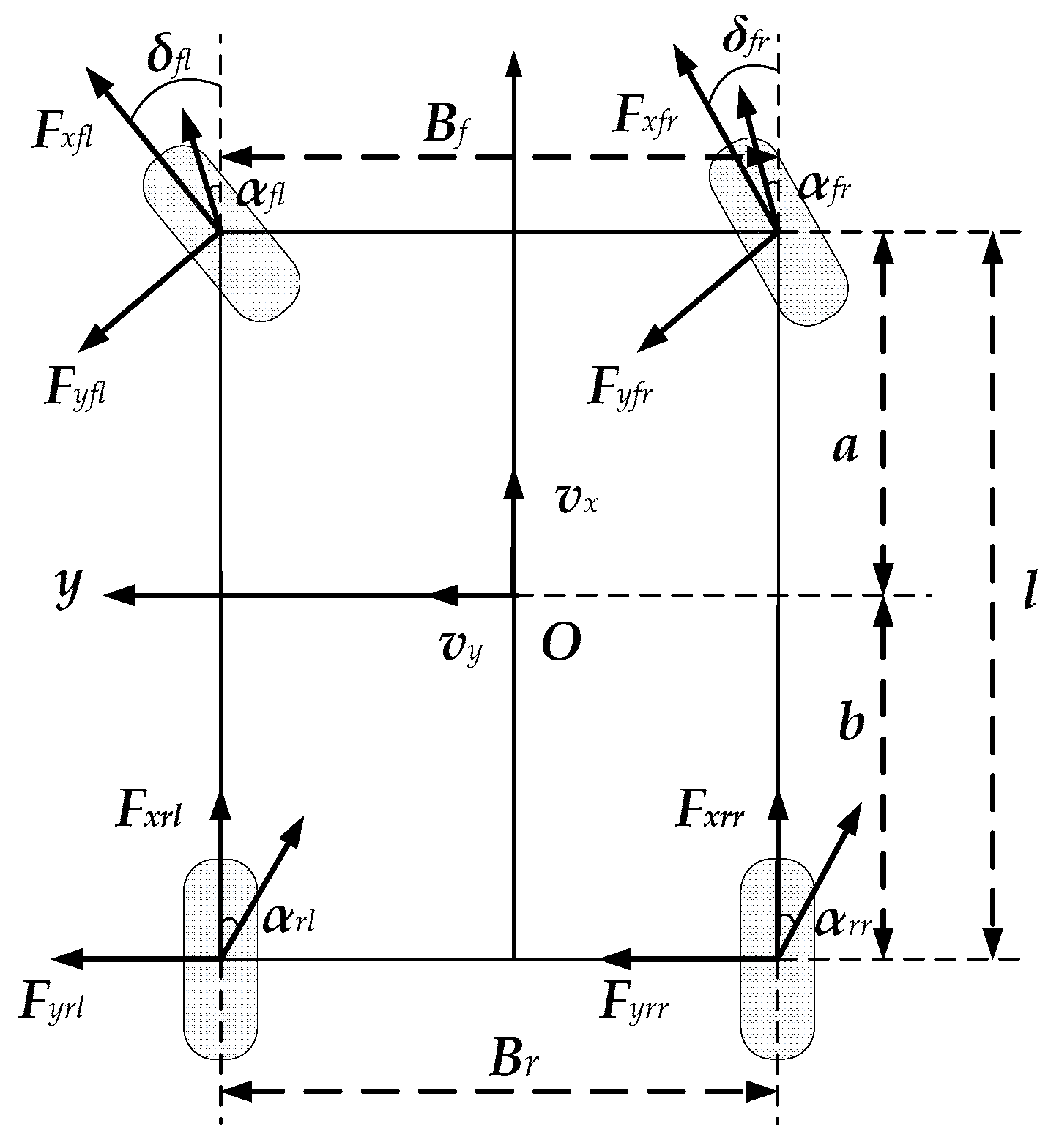
2.1. Seven Degrees of Freedom Vehicle Model

The nonlinear vehicle model described in this paper makes the following assumptions [26]: (1) the vehicle is only considered to move parallel to the ground; (2) the origin of the vehicle coordinate system coincides with the centroid point of the vehicle; and (3) we ignore the influence of longitudinal rolling resistance on the vehicle state. The nonlinear vehicle model studied in this paper is shown in Figure 2; a is the distance from the center of mass to the front axle; b is the distance from the center of mass to the rear axle; l = a + b is the distance from the front axle to the rear axle; B_f is the front wheel track; B_r is the rear wheel track; α_ij is the tire sideslip angle; F_xij is the longitudinal force of the tire; F_yij is the lateral force of the tire; δ_ij is the front wheel steering angle; v_x is the velocity of the center of mass along the x-axis; and v_y is the velocity of the center of mass along the y-axis. Among them, ij is fl, fr, rl, rr, which denote front left, front right, back left, and back right, and ij denotes this in the following model.

The longitudinal force balance equation:

$$\begin{array}{cc}\hfill m(\stackrel{•}{v_x}-{\omega }_r\cdot v_y)& =F_{xfl}\cos {\delta }_{fl}+F_{xfr}\cos {\delta }_{fr}-F_{yfl}\sin {\delta }_{fl}\hfill \\ & -F_{yfr}\sin {\delta }_{fr}+F_{xrl}+F_{xrr}-F_w\hfill \end{array}$$

(1)

The lateral force balance equation:

$$m(\stackrel{•}{v_y}+{\omega }_r\cdot v_x)=F_{xfl}\sin {\delta }_{fl}+F_{xfr}\sin {\delta }_{fr}+F_{yfl}\cos {\delta }_{fl}+F_{yfr}\cos {\delta }_{fr}+F_{yrl}+F_{yrr}$$

(2)

The moment balance equation around the z-axis:

$$\begin{array}{cc}\hfill I_z\cdot \stackrel{•}{{\omega }_r}& =a(F_{xfl}\sin {\delta }_{fl}+F_{xfr}\sin {\delta }_{fr}+F_{yfl}\cos {\delta }_{fl}+F_{yfr}\cos {\delta }_{fr})\hfill \\ & +\frac{B_f}{2}(F_{xfr}\cos {\delta }_{fr}-F_{xfl}\cos {\delta }_{fl})+\frac{B_f}{2}(F_{yfl}\sin {\delta }_{fl}-F_{yfr}\sin {\delta }_{fr})\hfill \\ & +(F_{xrr}-F_{xrl})\frac{B_r}{2}-(F_{yrl}+F_{yrr})b\hfill \end{array}$$

(3)

The absolute acceleration of the vehicle’s center of mass on the x-axis of the vehicle coordinate system:

$$a_x=\stackrel{•}{v_x}-{\omega }_r\cdot v_y$$

(4)

The absolute acceleration of the vehicle’s center of mass on the y-axis of the vehicle coordinate system:

$$a_y=\stackrel{•}{v_y}-{\omega }_r\cdot v_x$$

(5)

The vehicle sideslip angle of the center of mass:

$$\beta =\arctan \left(v_y/v_x\right)$$

(6)

The vertical load equation for each tire:

$$\begin{array}{l}{F}_{zfl(r)}=mg\frac{b}{2l}-m{a}_x\frac{h_g}{2l}\mp m{a}_y\frac{h_g}{B_f}\cdot \frac{b}{l}\\ F_{zrl(r)}=mg\frac{a}{2l}+m{a}_x\frac{h_g}{2l}\mp m{a}_y\frac{h_g}{B_r}\cdot \frac{a}{l}\end{array}$$

(7)

The vehicle sideslip angle equation for each tire:

$$\begin{array}{l}{\alpha }_{fl(r)}={\delta }_{fl(r)}-\arctan (\frac{v_y + a \cdot {\omega }_r}{v_x - \frac{B_f}{2} \cdot {\omega }_r})\\ {\alpha }_{rl(r)}= -\arctan (\frac{v_y - b \cdot {\omega }_r}{v_x - \frac{B_r}{2} \cdot {\omega }_r})\end{array}$$

(8)

The longitudinal velocity of each wheel center in the wheel coordinate system:

$$\begin{array}{l}{v}_{fl(r)}=(v_x\mp \frac{B_f}{2}\cdot {\omega }_r)\cos {\delta }_{fl(r)}+(v_y+a\cdot {\omega }_r)\sin {\delta }_{fl(r)}\\ v_{rl(r)}=v_x\mp \frac{B_r}{2}\cdot {\omega }_r\end{array}$$

(9)

The slip rate equation for each wheel:

$${\lambda }_{\mathrm{ij}}=\frac{{\Omega }_{ij}\cdot R-v_{ij}}{{\Omega }_{ij}\cdot R}=1-\frac{v_{ij}}{{\Omega }_{ij}\cdot R}$$

(10)

In the above formulas, F_w is the vehicle air resistance. β is the sideslip angle of the center of mass; ω_r is the yaw rate; R is the diameter of the tire; h_g is the distance from the center of mass to the ground; I_z is the moment of inertia of the entire vehicle around the z-axis; m is the mass of the entire vehicle; F_zij is the tire vertical force; a_x is the absolute acceleration of the vehicle’s center of mass on the x-axis of the vehicle coordinate system; and a_y is the absolute acceleration of the vehicle’s center of mass on the y-axis of the vehicle coordinate system. v_ij is the longitudinal velocity of each wheel center in the wheel coordinate system; Ω_ij is the wheel angular velocity in the wheel coordinate system; and λ_ij is the wheel slip rate.

2.2. Magic Formula

The Magic Formula uses the trigonometric function combination formula to fit the experimental tire data, and a set of formulas with the same form can completely express the longitudinal force and lateral force. The results can be obtained via data fitting or through looking up the table. The formula is suitable for product design, vehicle dynamic simulation, and test comparison, as these require an accurate description of the tire mechanical properties [27,28].

From the Magic Formula, the relationship between the tire force and the sideslip angle, the slip rate, and the ground vertical load on the tire is obtained as follows [29]:

$$\left\{\begin{array}{l}y(x)=D\sin \left\{C\arctan \left[Bx-E(Bx-\arctan Bx)\right]\right\}\\ Y(x)=y(x)+S_v\\ x=X+S_h\end{array}\right.$$

(11)

Among them:

$$\begin{gathered} D=a_1{F}_{zij}^2+a_2{F}_{zij}; E=a_7{F}_{zij}^2+a_8{F}_{zij}+a_9; \\ {S}_h=a_{10}\cdot \gamma ; S_v=(a_{11}{F}_{zij}^2+a_{12}{F}_{zij})\cdot \gamma \end{gathered}$$

(12)

The longitudinal force condition:

$$B\cdot C\cdot D=a_3\sin [a_4\arctan (a_5{F}_{zij})]\cdot (1-a_6\left|\gamma \right|)$$

(13)

The lateral force condition:

$$B\cdot C\cdot D=(a_3{F}_{zij}^2+a_4{F}_z)\cdot e^{-a_{12}\cdot F_{zij}}$$

(14)

In the above formulas, Y(x) is the longitudinal force or lateral force; X is the tire sideslip angle or longitudinal slip rate; D is the peak factor; B is the stiffness factor; C is the curve shape factor, which is taken as a constant; E is the curvature factor of the curve; S_h is the horizontal drift of the curve; S_v is the vertical drift of the curve; γ is the wheel camber angle; and a₁…a₁₂ are the fitting parameters.

3. Normalized Tire Force

For the estimation of the road adhesion coefficient, the Dugoff tire model expresses the mathematical relationship between the tire force and adhesion coefficient, which can meet the real-time detection, complexity, and model accuracy presented in the vehicle parameter estimation research [30,31]. The longitudinal force and lateral force of the tire can be expressed as follows:

$$\left\{\begin{array}{l}{F}_{xij}={\mu }_{ij}{F}_{\mathrm{z}ij}{C}_x\frac{{\lambda }_{ij}}{1-{\lambda }_{ij}}f(M)\\ F_{yij}={\mu }_{ij}{F}_{\mathrm{z}ij}{C}_y\frac{\tan {\alpha }_{ij}}{1-{\lambda }_{ij}}f(M)\end{array}\right.$$

(15)

$$f(M)=\left\{\begin{array}{l}(2-M)M,M<1\\ 1,M\ge 1\end{array}\right.$$

(16)

$$M=\frac{(1-{\lambda }_{ij})(1-\epsilon v_x\sqrt{{(C_x{\lambda }_{ij})}^2+{(C_y\tan {\alpha }_{ij})}^2})}{2\sqrt{{(C_x{\lambda }_{ij})}^2+{(C_y\tan {\alpha }_{ij})}^2}}$$

(17)

In the formula, C_x and C_y are, respectively, the longitudinal stiffness and cornering stiffness of the tire, and the tire stiffness can be obtained through the following method: Install the tire on the testing equipment, adjust the tire pressure to the standard tire pressure, continuously adjust the tire angle from different directions, record the tire force, draw the tire lateral angle curve, and calculate the tire stiffness. λ_ij is the wheel slip rate, and the parameter is obtained as follows: accelerate and brake the vehicle on the testing equipment, measure the relative displacement between the tire and the ground, and obtain the slip rate curve. The boundary value M > 1 indicates that the tire is in a linear interval, and M ≤ 1 indicates that the tire is in a nonlinear interval. ε is the speed influence factor, which corrects the influence of the tire slip speed on the tire longitudinal force. ε is determined by boundary condition M and adjusted in a timely manner. μ_ij is the road adhesion coefficient.

In order to facilitate the implementation of the estimation algorithm, Equation (15) can be simplified into a normalized form:

$$\left\{\begin{array}{l}{F}_{xij}={\mu }_{ij}{F}_{xij}{}^0={\mu }_{ij}{F}_{\mathrm{z}ij}{C}_x\frac{{\lambda }_{ij}}{1-{\lambda }_{ij}}f(M)\\ F_{yij}={\mu }_{ij}{F}_{yij}{}^0={\mu }_{ij}{F}_{\mathrm{z}ij}{C}_y\frac{{\lambda }_{ij}}{1-{\lambda }_{ij}}f(M)\end{array}\right.$$

(18)

In above formulas, F_xij⁰ and F_yij⁰ are, respectively, the tire normalized longitudinal force and lateral force, which are independent of the road adhesion coefficient. This facilitates the design of the estimation algorithm and is beneficial for estimating the road adhesion coefficient.

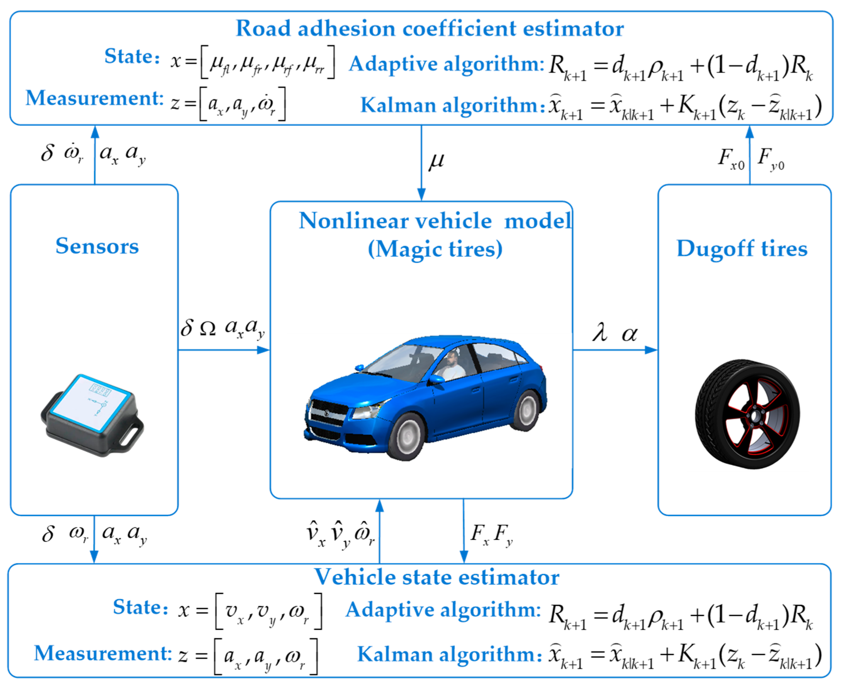
4. Higher-Order Cubature Kalman Filter Design

4.1. Vehicle State Estimation Algorithm

According to the nonlinear vehicle dynamics model, the vehicle state is estimated. For the general nonlinear system, the state estimation model can be expressed as

$$\left\{\begin{array}{l}\dot{x}(t)=f(x(t),u(t))+w(t)\\ \dot{z}(t)=h(x(t),u(t))+v(t)\end{array}\right.$$

(19)

In the formula, w(t) and v(t) are, respectively, the process noise and measurement noise of the system, which conform to Gaussian distribution and are independent of each other.

The state vector of the vehicle state estimator is defined as x_c(t) = [v_x,v_y,ω_r]^T, and the estimated state variable x_c(t) is fed back to the vehicle calculation module in Figure 1. The measurement vector of the vehicle state estimator is defined as z_c(t) = [a_x,a_y,ω_r]^T; the input vector of the vehicle state estimator is defined as u_c(t) = [δ, F_xij, F_yij]^T, where F_xij and F_yij are calculated by the nonlinear vehicle dynamics model and the Magic Formula tire model. According to Formulas (1)–(6), the state equation and measurement equation for vehicle state estimation are established.

The state equation of the vehicle estimator is established:

$${\dot{x}}_c(t)=\left[\begin{array}{ccc}\begin{array}{l}0\\ -{\omega }_r\\ 0\end{array}& \begin{array}{l}{\omega }_r\\ 0\\ 0\end{array}& \begin{array}{l}0\\ 0\\ 0\end{array}\end{array}\right]\left[\begin{array}{c}{v}_x\\ \begin{array}{l}{v}_y\\ {\omega }_r\end{array}\end{array}\right]+\left[\begin{array}{c}{\Delta }_1\\ \begin{array}{l}{\Delta }_2\\ {\Delta }_3\end{array}\end{array}\right]-\left[\begin{array}{l}\raisebox{1ex}{$1$}\!\left/ \!\raisebox{-1ex}{$m$}\right.\\ 0\\ 0\end{array}\right]F_w(t)+w(t)$$

(20)

In the formula,

$$\begin{gathered} {\Delta }_1=\frac{1}{m}(F_{xfl}\cos {\delta }_{fl}+F_{xfr}\cos {\delta }_{fr}-F_{yfl}\sin {\delta }_{fl}-F_{yfr}\sin {\delta }_{fr}+F_{xrl}+F_{xrr}) \\ {\Delta }_2=\frac{1}{m}(F_{xfl}\sin {\delta }_{fl}+F_{xfr}\sin {\delta }_{fr}+F_{yfl}\cos {\delta }_{fl}+F_{yfr}\cos {\delta }_{fr}+F_{yrl}+F_{yrr}) \\ \begin{array}{cc}\hfill {\Delta }_3& =\frac{1}{I_z}[a(F_{xfl}\sin {\delta }_{fl}+F_{xfr}\sin {\delta }_{fr}+F_{yfl}\cos {\delta }_{fl}+F_{yfr}\cos {\delta }_{fr})+\hfill \\ & \frac{B_f}{2}(F_{xfr}\cos {\delta }_{fr}-F_{xfl}\cos {\delta }_{fl})+\frac{B_f}{2}(F_{yfl}\sin {\delta }_{fl}-F_{yfr}\sin {\delta }_{fr})\hfill \\ & +(F_{xrr}-F_{xrl})\frac{B_r}{2}-(F_{yrl}+F_{yrr})b]\hfill \end{array} \end{gathered}$$

(21)

The measurement equation of the vehicle estimator is established:

$$z_c(t)=\left[\begin{array}{ccc}\begin{array}{l}0\\ 0\\ 0\end{array}& \begin{array}{l}0\\ 0\\ 0\end{array}& \begin{array}{l}0\\ 0\\ 1\end{array}\end{array}\right]\left[\begin{array}{c}{v}_x\\ \begin{array}{l}{v}_y\\ {\omega }_r\end{array}\end{array}\right]+\left[\begin{array}{c}{\Delta }_1\\ \begin{array}{l}{\Delta }_2\\ 0\end{array}\end{array}\right]-\left[\begin{array}{l}\raisebox{1ex}{$1$}\!\left/ \!\raisebox{-1ex}{$m$}\right.\\ 0\\ 0\end{array}\right]F_w(t)+v(t)$$

(22)

4.2. Road Adhesion Coefficient Estimation Algorithm

The road adhesion coefficient estimation algorithm estimates the road adhesion coefficient in real time, and the state estimation model is expressed in accordance with Equation (19).

If we take the adhesion coefficient of four wheels as the state vector of the road adhesion coefficient estimator x_p(t) = [μ_fl,μ_fr,μ_rl,μ_rr]^T; the longitudinal acceleration, lateral acceleration and yaw rate of the vehicle, measured via sensors, are used for the measurement vector of the road adhesion coefficient estimator z_p(t) = [a_x, a_y, $\stackrel{•}{{\omega }_r}$]^T; the front wheel angle and the normalized longitudinal and lateral forces of each wheel are used as the input vector of the road adhesion coefficient estimator: u_c(t) = [δ_ij, Fx_ij⁰, Fy_ij⁰]^T.

In a short period of time, the road adhesion coefficient can be regarded as constant. The state equation and measurement equation for the road adhesion coefficient estimator are as follows:

The state equation for the road adhesion coefficient estimator is established:

$$x_p(t)=\left[\begin{array}{cccc}\begin{array}{l}1\\ 0\\ 0\\ 0\end{array}& \begin{array}{l}0\\ 1\\ 0\\ 0\end{array}& \begin{array}{l}0\\ 0\\ 1\\ 0\end{array}& \begin{array}{l}0\\ 0\\ 0\\ 1\end{array}\end{array}\right]\left[\begin{array}{c}{\mu }_{fl}\\ {\mu }_{fr}\\ {\mu }_{rl}\\ {\mu }_{rr}\end{array}\right]+w(t)$$

(23)

$$z_p(t)=\left[\begin{array}{cccc}\begin{array}{l}{h}_{11}\\ h_{21}\\ h_{31}\end{array}& \begin{array}{l}{h}_{12}\\ h_{22}\\ h_{32}\end{array}& \begin{array}{l}{h}_{13}\\ h_{23}\\ h_{33}\end{array}& \begin{array}{l}{h}_{14}\\ h_{24}\\ h_{34}\end{array}\end{array}\right]\left[\begin{array}{c}{\mu }_{fl}\\ {\mu }_{fr}\\ {\mu }_{rl}\\ {\mu }_{rr}\end{array}\right]-\left[\begin{array}{l}\raisebox{1ex}{$1$}\!\left/ \!\raisebox{-1ex}{$m$}\right.\\ 0\\ 0\end{array}\right]F_w(t)+v(t)$$

(24)

In the formula,

$$\begin{gathered} h_{11}=\frac{F_{xfl}{}^0\cos {\delta }_{fl}-F_{yfl}{}^0\sin {\delta }_{fl}}{m}; h_{13}=\frac{F_{xrl}{}^0}{m}; \\ {h}_{12}=\frac{F_{xfr}{}^0\cos {\delta }_{fr}-F_{yfr}{}^0\sin {\delta }_{fr}}{m}; h_{14}=\frac{F_{xrr}{}^0}{m}; \\ {h}_{21}=\frac{F_{xfl}{}^0\sin {\delta }_{fl}+F_{yfl}{}^0\cos {\delta }_{fl}}{m}; h_{23}=\frac{F_{yrl}{}^0}{m}; \\ {h}_{22}=\frac{F_{xfr}{}^0\sin {\delta }_{fr}+F_{yfr}{}^0\cos {\delta }_{fr}}{m}; h_{24}=\frac{F_{yrr}{}^0}{m}; \\ {h}_{31}=\frac{2a(F_{xfl}{}^0\sin {\delta }_{fl}+F_{yfl}{}^0\cos {\delta }_{fl})+2a(F_{xfl}{}^0\sin {\delta }_{fl}+F_{yfl}{}^0\cos {\delta }_{fl})}{2I_z}; \\ {h}_{32}=\frac{2a(F_{xfr}{}^0\sin {\delta }_{fr}+F_{yfr}{}^0\cos {\delta }_{fr})+B_f(F_{xfr}{}^0\cos {\delta }_{fr}-F_{yfr}{}^0\sin {\delta }_{fr})}{2I_z}; \\ {h}_{33}=\frac{-B_r{F}_{xrl}{}^0-2b{F}_{yrl}{}^0}{2I_z}; h_{34}=\frac{B_r{F}_{xrr}{}^0-2b{F}_{yrr}{}^0}{2I_z}. \end{gathered}$$

(25)

4.3. Design GHCKF/AGHCKF Filter

Considering the discrete nonlinear system in the form of Equation (16), the GHCKF algorithm is used to solve the integral on the real domain Rⁿ:

$$I(g)={\displaystyle {\int }_{R^n}g(x)}\exp (-x^{T}x)dx$$

(26)

We select the first, second, and third G-trajectories to form the generalized fifth-order cubature integral formula, transform it to the standard Gaussian distribution, and then obtain the following formula [32,33]:

$$\begin{array}{cc}\hfill I(g)& ={\displaystyle {\int }_{R^n}g(x)}N(x;0,I)dx\hfill \\ & =\frac{1}{\sqrt{{\pi }^n}}{\displaystyle {\int }_{R^n}g(\sqrt{2}x)}\exp (-x^{T}x)dx\hfill \\ & =(1-\frac{(7-n)n}{18})g(\left[0\right])+\frac{4-n}{18}{\displaystyle \sum _{i=1}^{2n}g({\left[\sqrt{3}\right]}_i)}+\hfill \\ & \frac{1}{36}{\displaystyle \sum _{i=1}^{2n(n-1)}g({\left[\sqrt{3},\sqrt{3}\right]}_i)}\hfill \\ & ={\displaystyle \sum _{i=1}^{2n^2+1}{w}_{i}g({\xi }_i)}\hfill \end{array}$$

(27)

Among the values, the cubature points ξ_i and the weight values w_i are, respectively,

$${\xi }_i=\left\{\begin{array}{l}{\left[0\right]}_i,i=1;\\ {\left[\sqrt{3}\right]}_i,i=2,\cdots ,2n+1;\\ {\left[\sqrt{3},\sqrt{3}\right]}_i,i=2n+2,\cdots ,2n^2+1.\end{array}\right.$$

(28)

$$w_i=\left\{\begin{array}{l}(1-(7-n)n/18),i=1;\\ (4-n)/18,i=2,\cdots ,2n+1;\\ 1/36,i=2n+2,\cdots ,2n^2+1.\end{array}\right.$$

(29)

In the above equations, n is the number of state variables. We place Equations (27)–(29) under the Kalman filter framework to obtain the standard GHCKF algorithm [34]. The GHCKF algorithm for vehicle state estimation is as follows:

• Initialize state estimated values and error covariance:

$$\left\{\begin{array}{l}{\stackrel{⌢}{x}}_k=E(x_0)\\ P_k=E(x_0-{\stackrel{⌢}{x}}_k){(x_0-{\stackrel{⌢}{x}}_k)}^T\end{array}\right.$$

(30)

2.

Time update

(1) Calculate cubature points x_kⁱ (i = 1, 2, …, 2n² + 1):

$$S_k=SVD(P_k)$$

(31)

$${x_k}^i=S_k{\xi }_i+{\stackrel{⌢}{x}}_k$$

(32)

(2) Calculate cubature points propagated by the state equation x_k|k+1ⁱ:

$$x_{k|k+1}{}^i=f(x_k^i)$$

(33)

(3) Calculate the state estimation value at the current moment $\stackrel{⌢}{x}$_k|k+1ⁱ:

$${\stackrel{⌢}{x}}_{k|k+1}={\displaystyle \sum _1^{2n^2+1}{w}_i}{x}_{k|k+1}{}^i$$

(34)

(4) Calculate the prediction error covariance P_k|k+1:

$$P_{k|k+1}={\displaystyle \sum _1^{2n^2+1}{w}_i}(x_{k|k+1}{}^i-{\stackrel{⌢}{x}}_{k|k+1}){(x_{k|k+1}{}^i-{\stackrel{⌢}{x}}_{k|k+1})}^T+Q_k$$

(35)

In the equation, Q_k is the process noise covariance.

3.

Measurement update

(1) Calculate cubature points x_kⁱ (i = 1, 2, …, 2n² + 1):

$$S_{k+1}=SVD(P_{k|k+1})$$

(36)

$$x_{k+1}{}^i=S_{k+1}{\xi }_i+{\stackrel{⌢}{x}}_{k|k+1}$$

(37)

(2) Calculate cubature points propagated by the measurement equation z_k|k+1ⁱ:

$$z_{k|k+1}{}^i=h(x_{k+1}^i)$$

(38)

(3) Calculate the measurement prediction value at the current moment $\stackrel{⌢}{z}$_k|k+1ⁱ:

$${\stackrel{⌢}{z}}_{k|k+1}={\displaystyle \sum _1^{2n^2+1}{w}_i}{z}_{k|k+1}{}^i$$

(39)

(4) Calculate measurement error covariance P_k+1^zz and cross correlation covariance P_k+1^xz:

$$P_{k+1}^{zz}={\displaystyle \sum _1^{2n^2+1}{w}_i}(z_{k|k+1}{}^i-{\stackrel{⌢}{z}}_{k|k+1}){(z_{k|k+1}{}^i-{\stackrel{⌢}{z}}_{k|k+1})}^T+R_k$$

(40)

$$P_{k+1}^{xz}={\displaystyle \sum _1^{2n^2+1}{w}_i}(x_{k|k+1}{}^i-{\stackrel{⌢}{x}}_{k|k+1}){(z_{k|k+1}{}^i-{\stackrel{⌢}{z}}_{k|k+1})}^T$$

(41)

In the equation, R_k is the measurement of noise covariance.

4.

Update the filter gain matrix K_k+1, the state variable matrix $\stackrel{⌢}{x}$ _k+1, the error covariance matrix P_k+1:

$$K_{k+1}=P_{k+1}^{xz}{(P_{k+1}^{zz})}^{-1}$$

(42)

$${\stackrel{⌢}{x}}_{k+1}={\stackrel{⌢}{x}}_{k|k+1}+K_{k+1}(z_k-{\stackrel{⌢}{z}}_{k|k+1})$$

(43)

$$P_{k+1}=P_{k|k+1}-K_{k+1}{P}_{k+1}^{zz}{K}_{k+1}{}^T$$

(44)

In the formula, z_k is the measured value at the current time.

5.

Measurement noise covariance update:

In order to maintain the adaptive ability of the measurement noise variance matrix, the measurement noise covariance is updated via the exponential fading memory adaptive algorithm [35,36] to form the AGHCKF algorithm:

$$\begin{array}{cc}\hfill R_{k+1}& =d_{k+1}[(z_{k+1}-{\stackrel{⌢}{z}}_{k|k+1}){(z_{k+1}-{\stackrel{⌢}{z}}_{k|k+1})}^T\hfill \\ & -{\displaystyle \sum _0^{2n^2+1}{w}_i(z_{k|k+1}{}^i-{\stackrel{⌢}{z}}_{k|k+1})}{(z_{k|k+1}{}^i-{\stackrel{⌢}{z}}_{k|k+1})}^T]+(1-d_{k+1})R_k\hfill \end{array}$$

(45)

In the formula,

$$d_k=\frac{d_{k-1}}{d_{k-1}+s}; d_0=1; d_{\infty }=1-s,\hspace{0.33em}0<s<1.$$

(46)

In the above equation, s is called the fading factor.

5. Research Methods

This paper adopts a research and development method that combines simulation and experimentation. This paper selects typical operating conditions to conduct high-speed and low-speed simulation and experimental research on high- and low-adhesion road surfaces, respectively. Whether in simulation research or experimental research, the accuracy of the estimated results can be measured using the root-mean-square error (RMSE); the formula for the RMSE is as follows:

$$M=\sqrt{\frac{{\displaystyle \sum _{i=1}^n{\left(\widehat{\sigma }-{\sigma }_0\right)}^2}}{n_0}}$$

(47)

In the formula, M is the root-mean-square error; n₀ is the number of data; $\stackrel{⌢}{\sigma }$ is the evaluated value according to estimators; and σ₀ is the simulated value or sensor measurement value.

5.1. Simulation Design

Combined with the nonlinear vehicle dynamic model and the CKF/GHCKF/AGHCKF algorithm, a joint simulation platform is established to simulate a joint estimator of the vehicle state and the road adhesion coefficient. In this paper, a vehicle state estimator and road adhesion coefficient estimator are designed, respectively. The driving mode is selected as a rear in-wheel motor drive. The-double lane change condition and slalom condition are selected for the simulation analysis to verify the effectiveness of the joint algorithm. During the simulation process, Gaussian white noise is added to the measurement signal.

The double-lane change simulation is set to high speed, with a speed of 80 km/h, and the vehicle state estimation and road adhesion coefficient estimation are performed on high-adhesion roads, respectively; the road adhesion coefficient estimation is performed on low-adhesion surfaces. The high-adhesion road coefficient is set to 0.8, and the low-adhesion road coefficient is set to 0.5.

The slalom conditions are divided into a high-speed simulation and a low-speed simulation. The high-speed setting is 80 km/h, and the low-speed setting is 40 km/h. The simulated road adopts a joint road; the adhesion coefficient for the front 100 m road is set at 0.8, and the adhesion coefficient for the back 90 m road is set at 0.5. The vehicle state estimation and road adhesion coefficient estimation are performed during the low-speed slalom simulation; and the road adhesion coefficient estimation is only performed during the high-speed slalom simulation.

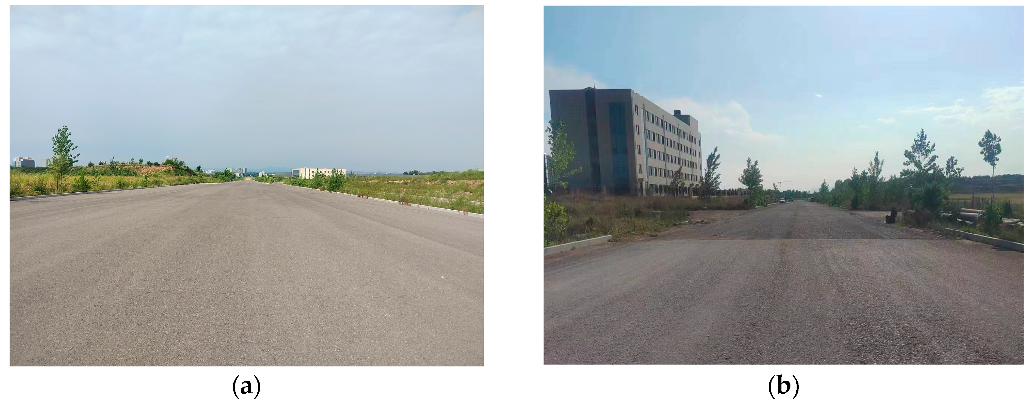
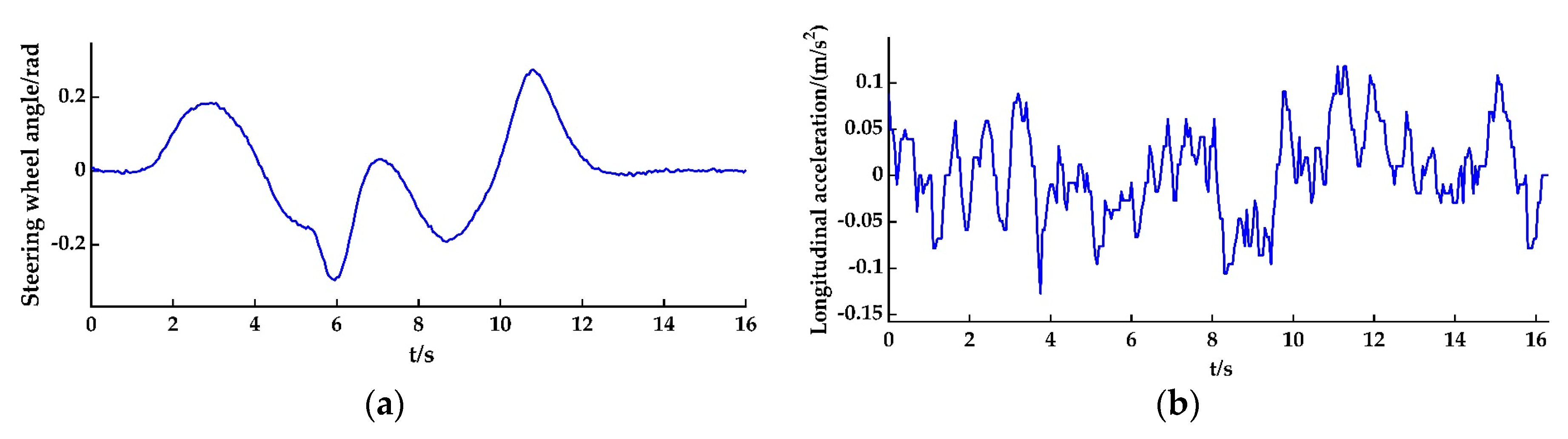
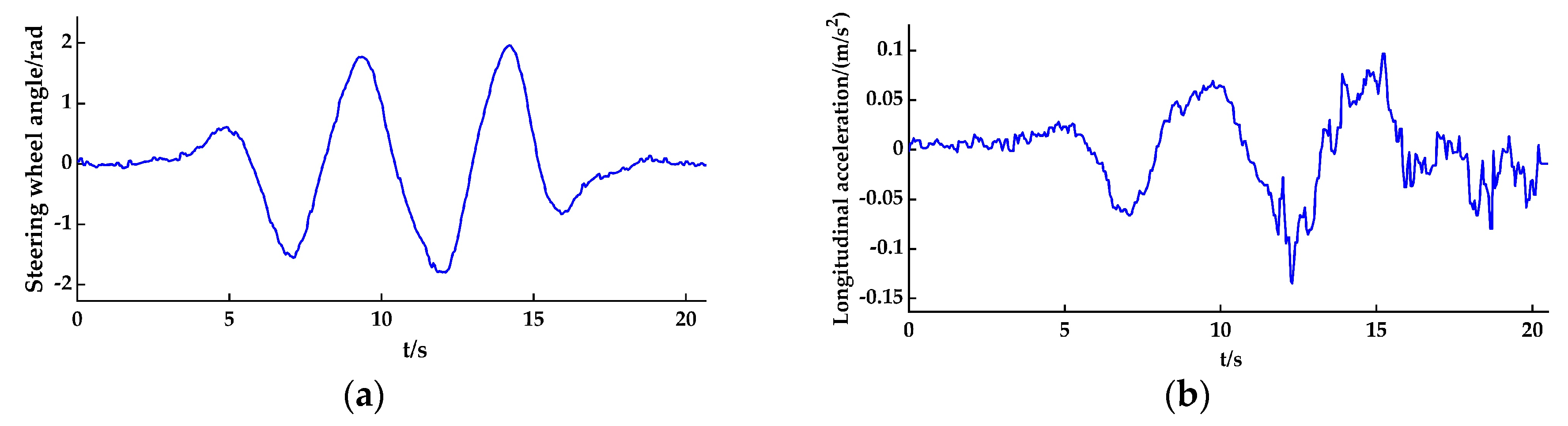
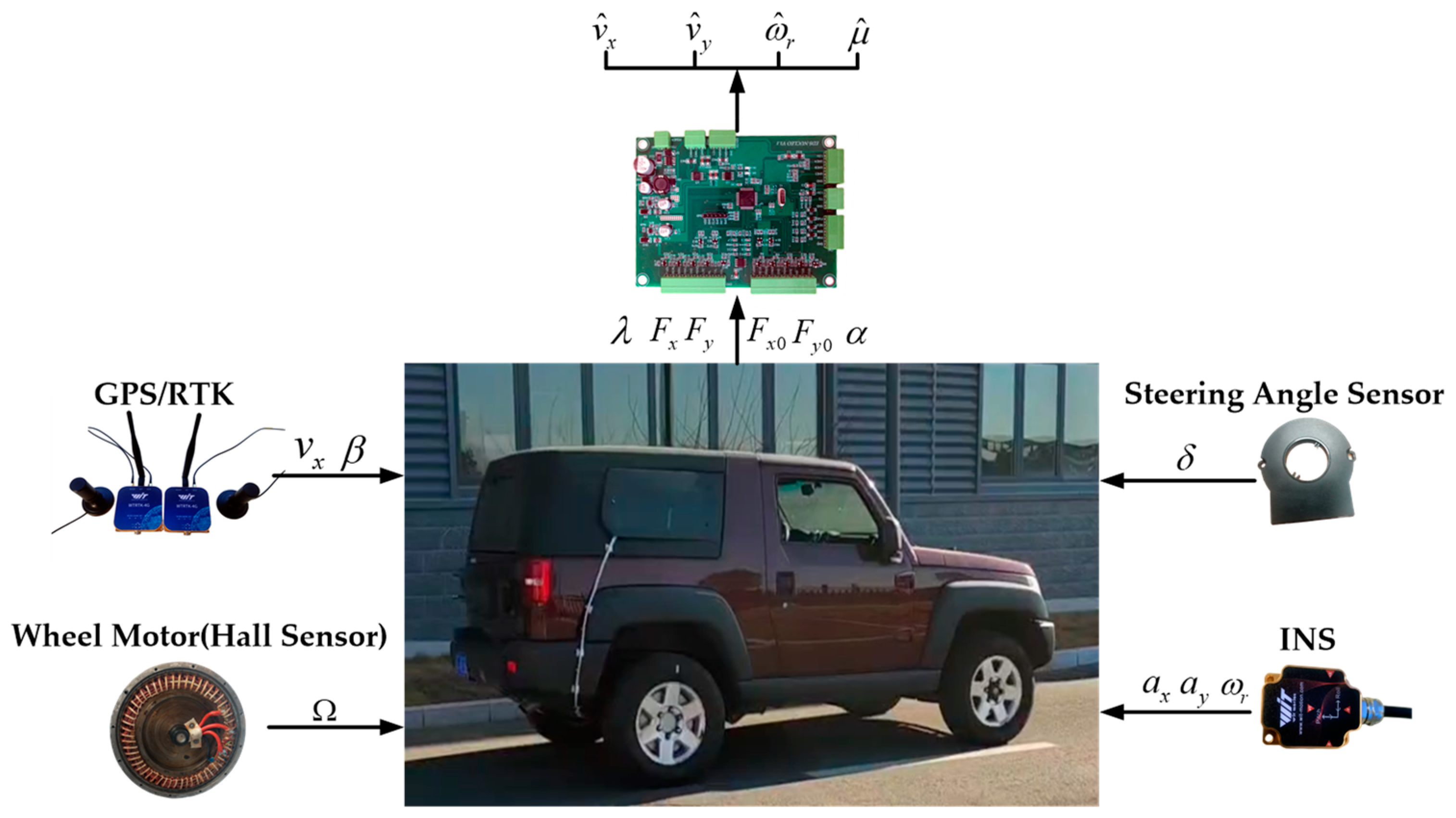
5.2. Experiment Design

In order to further verify the effectiveness of the joint estimator and compare the progressiveness of the CKF/GHCKF/AGHCKF algorithm, a modified vehicle driven by a rear in-wheel motor was used for experiments. As shown in Figure 3, the steering angle sensor collects the data of the steering wheel angle, the GPS/RTK module collects the data of the vehicle’s longitudinal velocity and heading angle, and the INS module collects the data of the lateral acceleration, lateral acceleration, yaw rate, and yaw angle. The Hall sensor in the hub motor can measure the wheel speed in real time. The lateral velocity cannot be directly measured. The collected heading angle, yaw angle, and longitudinal velocity are calculated to indirectly gain the lateral velocity. The upper computer software collects and saves the measurement data and inputs them into the controller. The built-in AGHCKF/GHCKF algorithm of the controller estimates the vehicle state and road adhesion coefficient in real time.

Considering the safety issues during the actual vehicle experimental process, in this paper, the double-lane change experiment was only conducted on high-adhesion coefficient roads, while the slalom experiment was conducted on a joint road at low speed.

As shown in Figure 4a, the test vehicle was driven on a new asphalt road surface at high speed (80 km/h) in the double-lane change experiment, and the driving data were collected via sensors to estimate the vehicle state and road adhesion coefficient. Referring to the relevant literature, the adhesion coefficient of asphalt pavement under high-speed driving conditions is approximately 0.6–0.7. As shown in Figure 4b, the test vehicle was driven on an asphalt–gravel joint road surface at low speed (40 km/h) in the slalom experiment, and the driving data were also collected via sensors to estimate the vehicle state and road adhesion coefficient. Referring to the relevant literature, the adhesion coefficient of the asphalt pavement under low-speed driving conditions is about 0.6–0.8, and the adhesion coefficient of the gravel road is about 0.4–0.7.

6. Result Analysis

6.1. Simulation Analysis

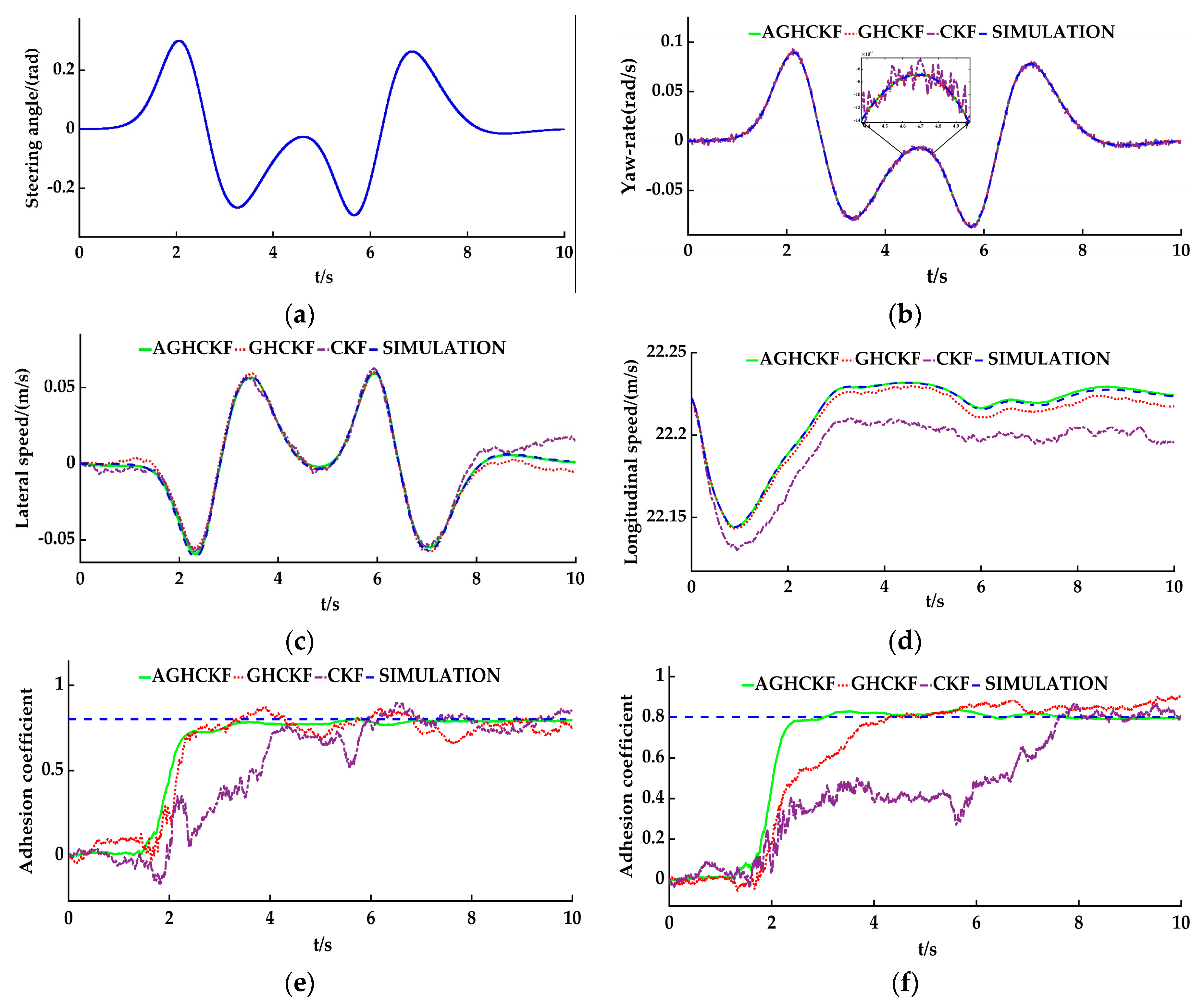
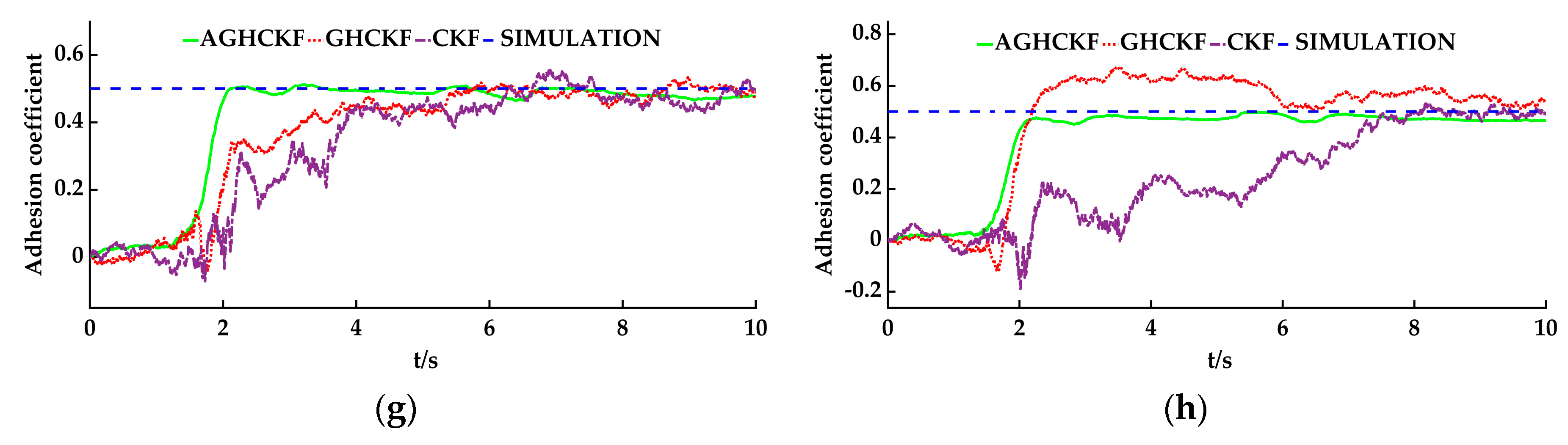
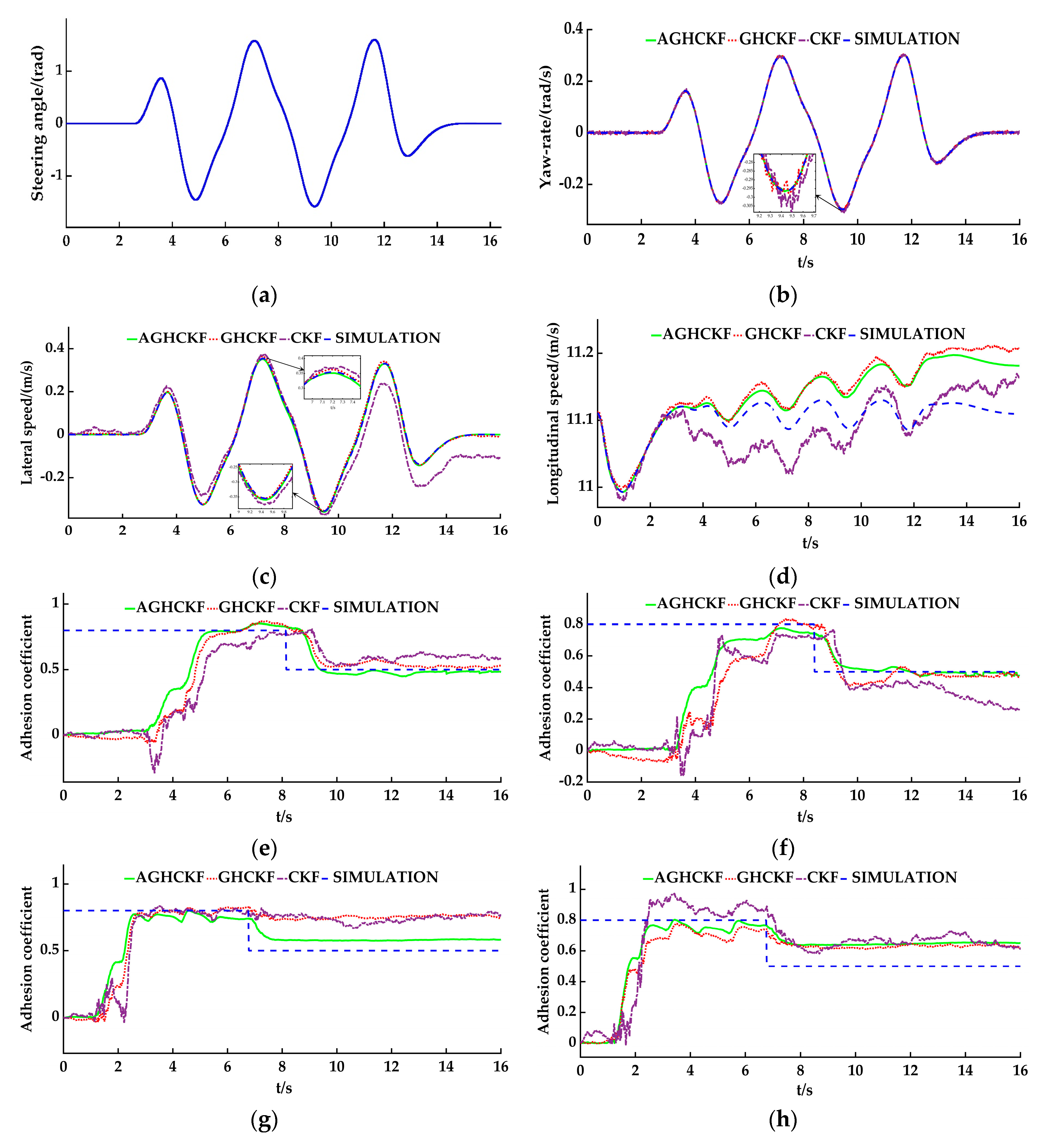
6.1.1. The Double-Lane Change Simulation

The sampling time interval is set to 0.005 s. The initial conditions of the vehicle state estimator are set as follows: the error covariance matrix P_c = 0.01 × eye(3); process noise covariance matrix Q_c = 0.1 × eye(3); and the measurement noise covariance matrix R_c = 0.1 × eye(3).

The initial conditions of the road adhesion coefficient estimator are set as follows: the error covariance matrix P_p = 0.01 × eye(4); process noise variance co-matrix Q_p = 0.01 × eye(4); and the measurement noise covariance matrix R_p = 0.1 × eye(3). In the simulation diagram, the blue line represents the simulated value, the red line represents the value estimated via GHCKF, the green line represents the value estimated via AGHCKF, and the purple line represents the value estimated via CKF.

To analyze the simulation results: Figure 5a shows the steering wheel angle change curve during the driving process of the vehicle along the double-lane change path. As the yaw rate is both the input of the measurement equation and the output of the state equation, the CKF, GHCKF, and AGHCKF algorithms can accurately track the measurement signal and estimate the yaw rate; however, in terms of the filtering effect and accuracy, as shown in Figure 5b, and the RMSE of the yaw rate, as shown in

Table 1. The RMSE of the double-lane change simulation.

Estimated Value	AGHCKFRMSE	GHCKFRMSE	CKFRMSE
The longitudinal velocity	0.0010	0.0039	0.0216
The lateral velocity	0.0011	0.0034	0.0051
The yaw rate	0.0001	0.0003	0.0015
The left rear wheel adhesion coefficient (μrl = 0.8)	0.3373	0.3394	0.4336
The right rear wheel adhesion coefficient (μrl = 0.8)	0.3375	0.3759	0.4414
The left rear wheel adhesion coefficient (μrl = 0.5)	0.1921	0.2218	0.2492
The right rear wheel adhesion coefficient (μrl = 0.5)	0.2010	0.2880	0.3365

, the AGHCKF is better than the GHCKF, and the GHCKF is better than the CKF. As shown in Figure 5c, the value estimated via AGHCKF can accurately track the lateral velocity simulation value, and the minimum RMSE value in the AGHCKF indicates the highest accuracy. However, in comparison with the simulation values, there are some errors in the values estimated via the GHCKF and CKF algorithms, especially at the positions of peaks and valleys. Further comparing the RMSE values of the two algorithms, the GHCKF is more accurate in estimating the lateral velocity than the CKF; as shown in Figure 5d, obviously, the AGHCKF algorithm is the most accurate for estimating the longitudinal velocity, while the GHCKF’s estimated value can differ from the simulated value by up to 0.005 m/s, while CKF’s estimated value can differ from the simulated value by up to 0.025 m/s; the CKF has the worst accuracy, as also confirmed via the RMSE value. In terms of filtering, the CKF is also the worst algorithm.

Compared with the simulation results for the road adhesion coefficient, according to Figure 5e–h, the trend of simulation results is consistent for both high-and low-road adhesion coefficients. The response time of AGHCKF in the figure is about 2 s, the response time of GHCKF is 3–4 s, and the response time of CKF is about 6–8 s. The curve of AGHCKF is smoother than that of GHCKF, and the curve of GHCKF is smoother than that of CKF. The RMSE values are shown in Table 1, AGHCKF_RMSE < GHCKF_RMSE < CKF_RMSE. That is, the AGHCKF has the fastest response, the best filtering effect, and the highest accuracy, followed by the GHCKF, and the CKF shows the worst performance in the three aspects.

6.1.2. The Slalom Simulation

The initial conditions of the vehicle state estimator and the road adhesion coefficient estimator are set the same as those in the double-lane change simulation, and the line type setting of the simulation diagram is also the same as in the double-lane change simulation.

To analyze the simulation results: Figure 6a shows the steering wheel angle change curve during the driving process of the vehicle along the slalom path. Similar to the double-lane change simulation, the simulated yaw rate is used as the input of the measurement equation and the output of the state equation at the same time. Therefore, Figure 6b shows that the values estimated via the AGHCKF, CHCKF, and CKF algorithms are very accurate. It can also be seen from the locally enlarged image that the filtering effect of the AGHCKF is the best, and that the CKF has the worst filtering effect; from Figure 6c, we can see that three algorithms can also estimate the lateral velocity. We can further observe the locally enlarged image, at the peaks and valleys of the lateral velocity curve, there are certain errors in the values estimated via GHCKF and CKF, but the error of the GHCKF is smaller than the error of the CKF. This result is consistent with the RMSE values for the lateral velocity in

Table 2. The RMSE of the slalom simulation.

Estimated Value	AGHCKFRMSE	GHCKFRMSE	CKFRMSE
The longitudinal velocity	0.0446	0.0521	0.0354
The lateral velocity	0.0042	0.0068	0.0613
The yaw rate	0.0004	0.0022	0.0029
The left rear wheel adhesion coefficient (vx = 40 km/h)	0.3910	0.4287	0.4441
The right rear wheel adhesion coefficient (vx = 40 km/h)	0.3912	0.4319	0.4407
The left rear wheel adhesion coefficient (vx = 80 km/h)	0.2685	0.3441	0.3413
The right rear wheel adhesion coefficient (vx = 80 km/h)	0.2759	0.2768	0.2963

. According to Figure 6d, both the AGHCKF and GHCKF algorithms undergo a process of divergence before stabilization when estimating the longitudinal velocity. The maximum error of the estimated value of the AGHCKF algorithm is about 0.06 m/s, while that of the CHCKF algorithm is about 0.08 m/s, and the RMSE value of the AGHCKF is smaller than the RMSE value of the GHCKF, meaning that the AGHCKF algorithm is superior to the CHCKF algorithm in terms of the estimation accuracy and filtering effect. The RMSE value of the CKF is smaller than the GHCKF, mainly because the CKF algorithm in the figure has been diverging, passing through the simulation curve, with many unstable approach points, leading to the CKF’s estimation of the longitudinal velocity being unreliable.

The AGHCKF and the GHCKF can handle high-order nonlinear characteristics and uncertainties in system dynamics, thereby achieving a higher filtering accuracy. Even so, it is still affected to some extent by the applied Gaussian white noise signal, so there is a certain error in the AGHCKF and the GHCKF curves in Figure 6d. The CKF is relatively weak in handling errors and noise in a nonlinear vehicle dynamics model, resulting in the accumulation and divergence of estimation errors when estimating the longitudinal velocity.

When driving at low speeds on the slalom line, the estimation effect of the road adhesion coefficient on the left rear wheel road surface is similar to that of the double-lane change simulation. The response time of AGHCKF in the figure is about 5 s, the response time of GHCKF is 6 s, and the response time of CKF is about 7 s. The curve of the AGHCKF is smoother than that of the GHCKF, and the curve of the GHCKF is smoother than that of the CKF. The RMSE values are shown in Table 2, AGHCKF_RMSE < GHCKF_RMSE < CKF_RMSE. So the AGHCKF has the best effect, the GHCKF takes the second place, and the CKF has the worst effect, as shown in Figure 6e,f and Table 2. It can also be seen that the estimated road adhesion coefficient is poor at around 0 to 6 s from the beginning. This is because the vehicle for Figure 6e,f is set to low speed, and the vehicle is in a straight and uniform state around 0 to 3 s. The state variables and measurements are constant, and the state equation and measurement equation of the estimator have not yet started to operate. Effective data are input around 3 s for operation, and convergence begins at 6 s to obtain an effective estimate of the road adhesion coefficient. On the other hand, the road state estimator indirectly uses the estimated values of the vehicle state estimator, and the estimation of road adhesion coefficient lags behind the estimation of the vehicle state; at the same time, the vehicle model and Magic Formula established have inherent errors, and the Dugoff tire model used for estimating the road adhesion coefficient also has errors, which accumulate and cause fluctuations in road adhesion coefficient estimation. In order to improve this problem, on the one hand, it is necessary to improve the mathematical models of the vehicle and tires, modify the structure, parameters, or initial conditions of the models to better match the actual system, and on the other hand, fully optimize the estimator structure and conduct multiple simulations to find the optimal control parameters and improve controller performance.

Figure 6g,h show the estimated results for the road adhesion coefficient during high-speed driving. The GHCKF and CKF have good estimates of the high-adhesion coefficient on the left rear wheel side, but cannot estimate the road adhesion coefficient on low-adhesion sections. On the right rear wheel side, it is possible to estimate the adhesion coefficient of high- and low-adhesion road surfaces within a certain range, and the filtering effect of the GHCKF is superior to that of the CKF. The AGHCKF algorithm can estimate the adhesion coefficient of the left and right rear wheel road surfaces within a certain accuracy range, the filtering effect is the best, and the estimation accuracy is the highest, as shown in Table 2. The difficulty in estimating the low adhesion road surface on the left rear wheel side via the GHCKF and CKF is mainly due to severe vehicle slip during high-speed slalom driving, and the insufficient accuracy in calculating the tire force on the left rear wheel. This also indirectly indicates that the AGHCKF has a strong anti-interference ability.

6.2. Experiment Analysis

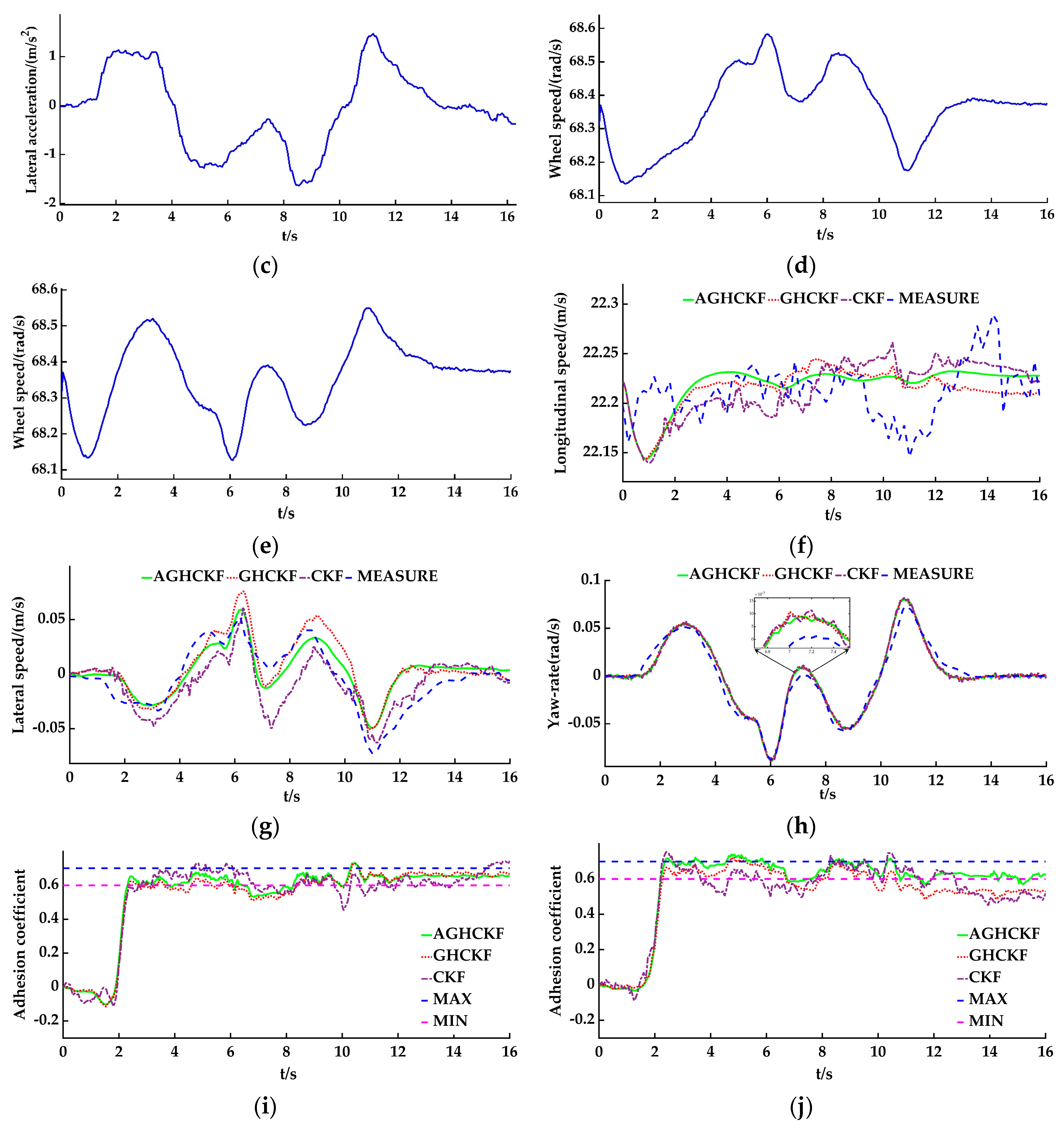
6.2.1. The Double-Lane Change Experiment

The sampling time interval of the GPS/RTK module is set to 0.05 s, and the sampling time of the INS is set to 0.2 s. Figure 7a shows the steering wheel angle change curve sampled by the angle sensor. Figure 7b,c are the longitudinal acceleration curve and lateral acceleration curve sampled by the INS module, and the wheel velocity curves are sampled by the Hall sensor, as shown in Figure 7d,e. The measurement data such as the longitudinal/lateral acceleration and yaw rate are transmitted to the built-in GHCKF and AGHCKF algorithm platforms of the controller, and the longitudinal velocity, lateral velocity, yaw rate and road adhesion coefficient are calculated and compared with the measured values. In Figure 7f–h, the blue line represents the direct and indirect measurement value of the sensor, the red line represents the estimated value of the GHCKF, the green line represents the estimated value of the AGHCKF, and the purple line represents the estimated value of the CKF. In Figure 7i,j, the blue line represents the upper limit of the road adhesion coefficient, and the pink line represents the lower limit.

The longitudinal acceleration fluctuates in a small range at the 0 scale line. The longitudinal acceleration curve, the lateral acceleration curve, and the two wheel speed curves change with the law of the double-lane change. The above curves fluctuate with the vehicle movement, and their changing rule is consistent with the theoretical analysis and conforms to the actual working conditions. As shown in Figure 7f and

Table 3. The RMSE of the double-lane change experiment.

Estimated Value	AGHCKFRMSE	GHCKFRMSE	Difference
The longitudinal velocity	0.0320	0.0339	0.0371
The lateral velocity	0.0163	0.0181	0.0202
The yaw rate	0.0064	0.0065	0.0068
The left rear wheel adhesion coefficient	0.2469	0.2500	0.2537
The right rear wheel adhesion coefficient	0.2335	0.2416	0.2392

, the AGHCKF, GHCKF and CKF algorithms can effectively track the longitudinal velocity of the vehicle and can effectively filter; the AGHCKF has the best overall effect, followed by the GHCKF and CKF. When the AGHCKF algorithm is used to estimate the lateral velocity, Figure 7g shows that the matching degree between the AGHCKF and the simulation curves is better than that for the GHCKF and CKF, and the accuracy is also the highest, as shown in Table 3. According to Figure 7h, the GHCKF, GHCKF and CKF can all accurately track the measured yaw rate. The locally enlarged image and RMSE values show that the filtering effect and estimation accuracy of the AGHCKF are higher than those of the GHCKF, and that those of the GHCKF are higher than those of the CKF. Figure 7i,j show the estimation curves of the road adhesion coefficient on the rear wheel drive side. Due to accumulation of the accuracy errors of the vehicle model, the errors of Magic Formula, the accuracy errors of the Dugoff tire model, and the errors of accuracy errors of measurement sensors, none of the algorithms cannot accurately estimate the road adhesion coefficient; they can only roughly estimate it within the coefficient range. The RMSE values are shown in Table 3, although AGHCKF_RMSE < CKF_RMSE < GHCKF_RMSE, the value estimated via the AGHCKF is more in the range of road adhesion coefficient than GHCKF, and that of the the GHCKF is more than the CKF. The response time of the three algorithms is similar. The curve of the AGHCKF is smoother than the GHCKF, and the curve of the GHCKF is smoother than the CKF. Overall, the AGHCKF has the best estimation effect, followed by the GHCKF, and the CKF is the worst.

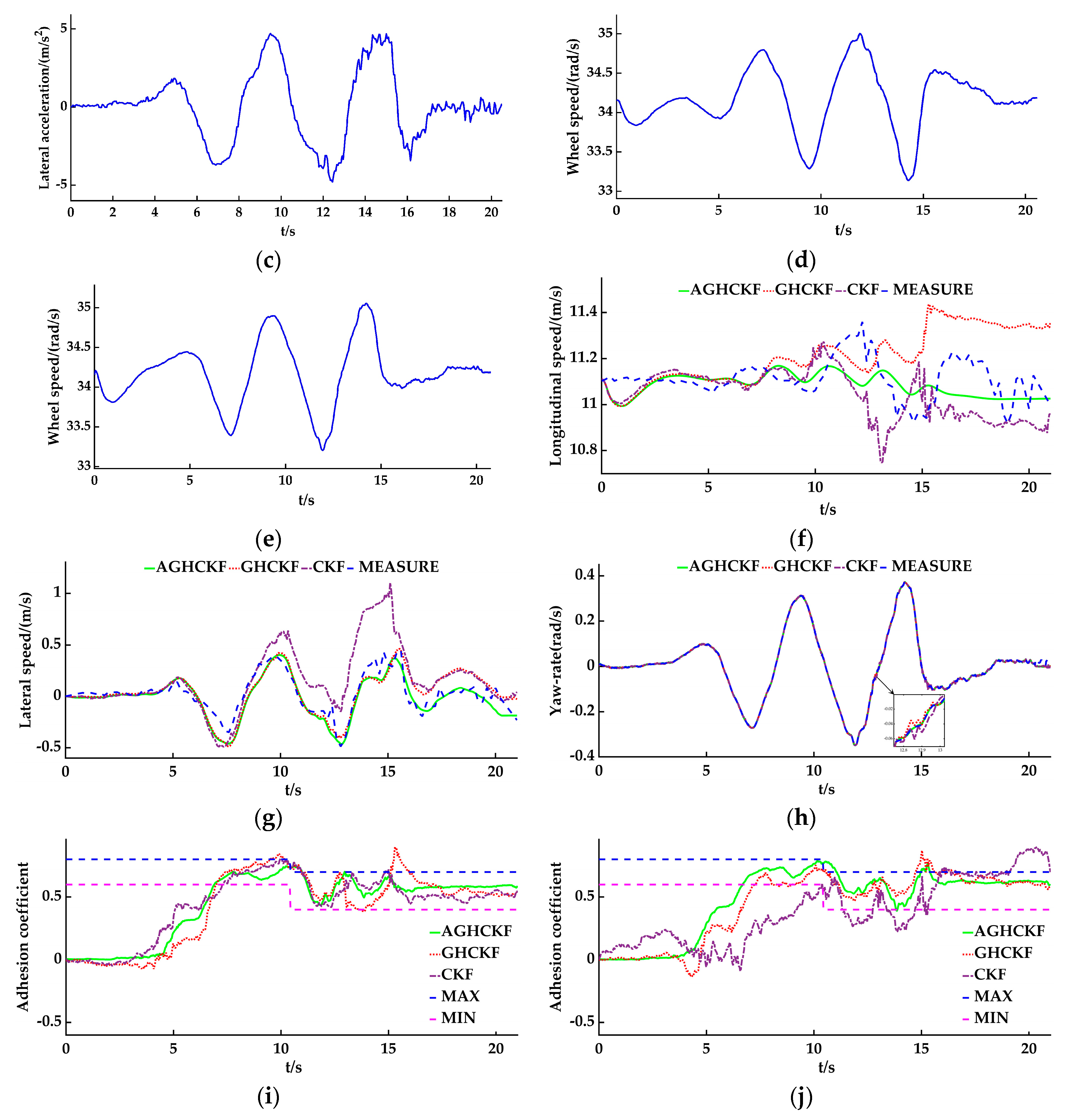
6.2.2. The Slalom Experiment

The low-speed slalom experiment was conducted on the asphalt–gravel joint road, and the sensor settings are the same as those in the double-lane change experiment. Figure 8a shows the steering wheel angle change curve sampled by the angle sensor. Figure 8b,c, respectively, show the lateral acceleration and longitudinal acceleration curves sampled by the INS module, and the wheel speed curves sampled by the Hall sensor, as shown in Figure 8d,e. For the first 12 s, when the vehicle was driving on an asphalt road, the measurement data were relatively stable. After 12 s, when the vehicle was driving on the gravel road surface, the data fluctuated significantly, which is in line with the actual working conditions of the joint road. We input the measurement data into the controller, and the GHCKF and AGHCKF algorithms in the controller calculate the longitudinal velocity, lateral velocity, yaw rate, and road adhesion coefficient, and then compare them with the measured values. The line type settings in the figures are the same as those in the double-lane change experiment.

As shown in Figure 8b–d, the results show that the longitudinal acceleration fluctuates within a small range of the 0 scale line, and the curves of the longitudinal acceleration, the lateral acceleration, and wheel speed change along with the slalom law. The experiment curves fluctuate with the vehicle’s movement, and their changing rule is consistent with the theoretical analysis and practical working conditions. As shown in Figure 8f, the GHCKF and CKF algorithms can effectively track the longitudinal velocity of the vehicle up until 12 s, but the error relatively increases in the latter seconds. The maximum estimated value of the GHCKF reaches 11.4 m/s, while the minimum estimated value of CKF reaches 10.7 m/s; according to

Table 4. The RMSE of the slalom experiment.

Estimated Value	AGHCKFRMSE	GHCKFRMSE	CKFRMSE
The longitudinal velocity	0.0199	0.0203	0.185
The lateral velocity	0.0881	0.1160	0.2456
The yaw rate	0.0041	0.0044	0.0051
The left rear wheel adhesion coefficient	0.3496	0.3896	0.3406
The right rear wheel adhesion coefficient	0.3404	0.3688	0.3983

, the accuracy of the GHCKF is much higher than that of the CKF. However, the AGHCKF algorithm can accurately follow the longitudinal velocity measurement values of the entire vehicle throughout the entire process, the filtering effect is significant, and the AGHCKF has the highest estimation accuracy. As shown in Figure 8g, compared with the CKF, the AGHCKF and GHCKF can more accurately track lateral velocity measurements, especially in the peak and valley of the curve, and during the running time after 10 s. The AGHCKF algorithm has a better filtering effect and a higher estimation accuracy than those of the GHCKF. In the above aspects, the GHCKF is again better than the CKF; as shown in Figure 8h, the AGHCKF, GHCKF, and CKF can all accurately track the measured values for the yaw rate. The local enlarged image and Table 4 show that the AGHCKF algorithm has the best filtering performance and highest estimation accuracy. The factors affecting the estimation of the adhesion coefficient are the same as those in the double-lane change experiment, and the adhesion coefficient can only be roughly estimated within the coefficient range. The response time of the AGHCKF in the figure is about 6–7 s, the response time of the GHCKF is 6–8 s, and the response time of the CKF is about 7–10 s. The curve of the AGHCKF is smoother than the GHCKF, and the curve of GHCKF is smoother than the CKF. The RMSE values are shown in Table 4, for the adhesion coefficient of the left rear wheel: CKF_RMSE <AGHCKF_RMSE < GHCKF_RMSE, and for the adhesion coefficient of the right rear wheel: AGHCKF_RMSE <GHCKF_RMSE < CKF_RMSE. Overall, compared to the GHCKF and CKF, the adhesion coefficient estimated values of the AGHCKF algorithm are relatively stable, both located in the upper and lower limits. And the AGHCKF algorithm responds the fastest of all.

7. Conclusions

This study uses a high-order algorithm to jointly estimate the vehicle state and road adhesion coefficient. Simulation analysis and experimental methods were used to verify the joint estimator of the vehicle state and road adhesion coefficient and, through further comparison among the GHCKF, AGHCKF, and CKF, the following conclusions can be obtained.

The experimental results are consistent with the simulation analysis; both the experimental and the simulation results indicate that the AGHCKF, GHCKF, and CKF algorithms can estimate state parameters such as the vehicle longitudinal speed, lateral speed and yaw rate, and can effectively estimate the road adhesion coefficient. However, after in-depth comparison, we conclude that the AGHCKF algorithm is superior to the GHCKF and CKF algorithms in terms of its response speed, estimation accuracy, and filtering effect; this reflects the effectiveness and robustness of the AGHCKF algorithm.

The joint estimator realizes the estimation of the vehicle state and road adhesion coefficient. The joint estimation method for the vehicle state and road adhesion coefficient proposed in this paper is feasible. According to the simulations and experiments, the vehicle state estimator can generally achieve an accurate estimation of the vehicle state, the road adhesion coefficient estimator can achieve an the effective estimation of the road adhesion coefficient, and the estimated value has always been within the effective range of the road adhesion coefficient; the estimated results can meet the requirements of vehicle dynamic simulation, control, and test.

This study innovatively proposes a method for the joint estimation of the vehicle state and road adhesion coefficient, introduced high-order Kalman and adaptive algorithms, and developed an advanced AGHCKF algorithm. The comparison of the results with those of the GHCKF and CKF shows that the AGHCKF can better adapt to the errors and noise of nonlinear systems, has a strong anti-interference ability, and has a good robustness and stability. The experimental data to some extent reflect the true engineering values. Comparing the estimated values with the measured values of sensors, the RMSE values are all less than 0.04. Among them, the AGHCKF has the smallest RMSE value, the most accurate estimation of vehicle status and road adhesion coefficient, the shortest response time, and the most stable data. Therefore, the AGHCKF algorithm has great advantages in the field of vehicle control.

References

1. Cha, Y.F.; Lu, X.L.; Chen, H.Q.; Yi, Y.C.; Wang, Y.Y. Vehicle trajectory tracking control based on road surface attachment coefficient estimation. Automot. Eng. 2023, 45, 1010–1039. [Google Scholar] [CrossRef]
2. Zhu, B.; Pu, Q.; Li, L.; Zhao, J.; Wu, J.; Deng, W.W. Vehicle longitudinal collision warning strategy based on road adhesive coefficient estimation. Automot. Eng. 2016, 38, 446–452. [Google Scholar] [CrossRef]
3. Ping, X.Y.; Li, L.; Cheng, S.; Wang, H.Y. Tire-road friction coefficient estimators for 4 WID electric vehicles on diverse road conditions. J. Mech. Eng. 2019, 55, 80–92. [Google Scholar] [CrossRef]
4. Zhang, X.; Liu, L.; Ma, X.J.; Zhang, Y.Y.; Chen, L. Driving force coordinated control of an 8x8 in-wheel motor drive vehicle with tire-road friction coefficient identification. Def. Technol. 2022, 18, 119–132. [Google Scholar] [CrossRef]
5. Wang, Y.; Geng, K.; Xu, L.; Ren, Y.; Dong, H.; Yin, G.D. Estimation of sideslip angle and tire cornering stiffness using fuzzy adaptive robust cubature Kalman filter. IEEE Trans. Syst. Man Cybern. 2020, 52, 1451–1462. [Google Scholar] [CrossRef]
6. Cheng, S.; Li, L.; Chen, J. Fusion algorithm design based on adaptive SCKF and integral correction for side-slip angle observation. IEEE Trans. Industr. Electr. 2017, 65, 5754–5763. [Google Scholar] [CrossRef]
7. Li, S.H.; Wang, G.Y.; Yang, Z.K.; Wang, X.W. Dynamic joint estimation of vehicle sideslip angle and road adhesion coefficient based on DRBF-EKF algorithm. Chin. J. Theor. Appl. Mech. 2022, 54, 1853–1865. [Google Scholar] [CrossRef]
8. Huang, B.; Fu, X.; Wu, S.; Huang, S. Calculation algorithm of tire-road friction coefficient based on limited-memory adaptive extended Kalman filter. Math. Probl. Eng. 2019, 2019, 1056269. [Google Scholar] [CrossRef]
9. Jin, X.J.; Yang, J.P.; Yin, G.D.; Wang, J.X.; Chen, N.; Lu, Y.B. Combined state and parameter observation of distributed drive electric vehicle via dual unscented Kalman filter. J. Mech. Eng. 2019, 55, 93–102. [Google Scholar] [CrossRef]
10. Jin, X.J.; Yang, J.P.; Li, Y.J.; Zhu, B.; Yin, G.D. Online estimation of inertial parameter for lightweight electric vehicle using dual unscented Kalman filter approach. IET Intell. Transp. Syst. 2020, 14, 412–422. [Google Scholar] [CrossRef]
11. Arasaratnam, I.; Haykin, S. Cubature Kalman filters. IEEE Trans. Autom. Control 2009, 54, 1254–1269. [Google Scholar] [CrossRef]
12. Arasaratnam, I.; Haykin, S.; Hurd, T.R. Cubature Kalman filtering for continuous-discrete systems: Theory and simulations. IEEE T Signal Process 2010, 58, 4977–4993. [Google Scholar] [CrossRef]
13. Wang, Y.; Yin, G.D.; Geng, K.K.; Dong, H.X.; Lu, Y.B.; Zhang, F.J. Tire lateral forces and sideslip angle estimation for distributed drive electric vehicle using noise adaptive cubature Kalman filter. J. Mech. Eng. 2019, 55, 103–112. [Google Scholar] [CrossRef]
14. Xing, D.X.; Wei, M.X.; Zhao, W.Z.; Wang, Y.; Wu, S.F. Vehicle state estimation based on adaptive volumetric particle filtering. J. Nanjing Univ. Aeronaut. Astronaut. 2020, 52, 445–453. [Google Scholar] [CrossRef]
15. Zhang, Z.D.; Zheng, L.; Li, Y.N.; Wu, X.; Yu, Y.H. Robust adaptive SCKF-based target state tracking for intelligent vehicles. J. Mech. Eng. 2021, 57, 181–193. [Google Scholar] [CrossRef]
16. Wu, H.; Chen, S.X.; Yang, B.F.; Chen, K. Robust cubature Kalman filter target tracking algorithm based on genernalized M-estiamtion. Acta Phys. Sin. 2015, 64, 456–463. [Google Scholar] [CrossRef]
17. Qi, D.L.; Feng, J.G.; Li, Y.B.; Wang, L.; Song, B. A Robust hierarchical estimation scheme for vehicle state based on maximum correntropy square-root cubature Kalman filter. Entropy 2023, 25, 453. [Google Scholar] [CrossRef]
18. Chen, X.; Li, S.; Zhao, W.; Cheng, S. Longitudinal-lateral-cooperative estimation algorithm for vehicle dynamics states based on adaptive square root cubature Kalman filter and similarity-principle. Mech. Syst. Signal Process. 2022, 176, 109162–109183. [Google Scholar] [CrossRef]
19. Mcnamee, J.; Stenger, F. Construction of fully symmetric numerical integration formulas. Numer. Mathmatik 1967, 10, 327–344. [Google Scholar] [CrossRef]
20. Su, B.Z.; Mu, R.J.; Long, T.; Cheng, C.; Cui, N.G. Performance Evaluation of HCKF and Its Application in Transfer Alignment. J. Astronaut. 2019, 40, 1313–1321. [Google Scholar]
21. Zhang, X.F.; Guo, C.; Qin, K.; Yao, B. High-degree cubature Kalman filter with colored measurement niose and its application. Comput. Eng. Appl. 2017, 53, 263–270. [Google Scholar] [CrossRef]
22. Li, W.; Hao, S.Y.; Huang, G.R.; Ma, S.J. Improved adaptive ADMCC-HCKF algorithm and application in SINS/CNS/GNSS integrated navigation. J. Electron. Meas. Instrum. 2021, 35, 79–85. [Google Scholar] [CrossRef]
23. Qin, K.; Dong, X.M.; Chen, Y.; Liu, Z.C.; Li, H.B. Huber-based robust generalized high-degree cubature Kalman filter. Control Decis. 2018, 3, 88–94. [Google Scholar] [CrossRef]
24. Hao, S.Y.; Lu, H.; Wei, X.; Xu, M.Q. Reduced high-degree strong tracking cubature Kalman filter and its application in inte-grated navigation system. Control Decis. 2019, 34, 2105–2114. [Google Scholar] [CrossRef]
25. Liu, Y.; Huang, P. A more general class of cubature Kalman filters. Comput. Eng. Appl. 2015, 51, 207–210. [Google Scholar] [CrossRef]
26. Yan, S.; Zhang, H.H.; Gao, C.; Li, Q.W. The linear three-degree-of-freedom vehicle model based on Simulink simula-tion. Intell. Comput. Appl. 2020, 10, 200–207. [Google Scholar]
27. Qiu, C.F.; Zhou, L.; Chen, R.Q.; Sun, X.Y.; Jia, C.H.; Qiu, J.W.; Zhang, C.; Yang, H.T. Calculation Method of Tire Longitudinal Slip Characteristic Parameters Based on Magic Formula. Tire Ind. 2021, 41, 607–611. [Google Scholar] [CrossRef]
28. Ružinskas, A.; Sivilevičius, H. Magic formula tyre model application for a tyre-ice interaction. Procedia Eng. 2017, 187, 335–341. [Google Scholar] [CrossRef]
29. Zheng, X.M.; Gao, X.W.; Zhao, Z.Z. Simulation analysis of tire dynamic based on “Magic Formula”. Mach. Electron. 2012, 9, 16–20. [Google Scholar] [CrossRef]
30. Zhang, L.; Shi, P.L.; Zhou, L.H.; Jiang, J.X.; Liang, M.L.; Hou, J.W. Estimation of vehicle sideslip angle based on Dugoff tire model. J. Guangxi Univ. 2021, 46, 1523–1532. [Google Scholar] [CrossRef]
31. Dugoff, H.; Fancher, P.S.; Segel, L. An analysis of tire action properties and their influence on vehicle dynamic performance. SAE Trans. 1970, 79, 1219–1243. [Google Scholar] [CrossRef]
32. Peng, Z.Y.; Xia, H.B.; Xu, Y.S. Adaptive generalized high-degree Cubature Kalman Filter based on target tracking. Comput. Eng. Appl. 2018, 54, 46–52. [Google Scholar] [CrossRef]
33. Zhang, X.C.; Teng, S.J. A New Derivation of the Cubature Kalman Filters. Asian J. Control 2014, 16, 1501–1510. [Google Scholar] [CrossRef]
34. Liu, D.; Chen, X.Y.; Xu, Y.; Liu, X.; Shi, C.F. Maximum correntropy generalized high-degree cubature Kalman filter with application to the attitude determination system of missile. Aerosp. Sci. Technol. 2019, 95, 105441. [Google Scholar] [CrossRef]
35. Yang, H.Z.; Wang, S.B.; He, H.L. Adaptive Cubature Kalman Filter Based on Unknown Noise Covariance. J. Air Force Eng. Univ. 2021, 22, 42–47. [Google Scholar] [CrossRef]
36. Ge, J.; Dong, H.B.; Liu, H.; Bai, M.M.; Qiu, X.Y.; Yuan, Z.W.; Liu, Y.H.; Zhu, J.; Zhang, H.Y. Real-time Reduction of Magnetic Noise Associated with Ocean Waves via Sage-Husa lgorithm for Towed Overhauser Marine Geomagnetic Sensor. Earth Sci. 2018, 43, 3792–3798. [Google Scholar] [CrossRef]
Figure 1. Schematic diagram for the joint estimation of the vehicle state and the road adhesion coefficient.
Applsci 13 10734 g001
Figure 2. The nonlinear dynamic vehicle model.
Applsci 13 10734 g002
Figure 3. The experiment principle and equipment.
Applsci 13 10734 g003
Figure 4. The experiment conditions. (a) The new asphalt pavement for the high-speed double-lane change experiment; and (b) the asphalt—gravel joint road for the low-speed slalom experiment.
Applsci 13 10734 g004
Figure 5. The results of the double−lane change simulation. (a) The steering angle; (b) the yaw rate; (c) the lateral velocity; (d) the longitudinal velocity; (e) the left rear wheel road adhesion coefficient with a high−adhesion road surface; (f) the right rear wheel road adhesion coefficient with a high−adhesion road surface; (g) the left rear wheel road adhesion coefficient with a low−adhesion road surface; and (h) the left rear wheel road adhesion coefficient with a low−adhesion road surface.
Applsci 13 10734 g005aApplsci 13 10734 g005b
Figure 6. The results of the slalom simulation on a joint road. (a) The steering angle; (b) the yaw rate; (c) the lateral velocity; (d) the longitudinal velocity; (e) the left rear wheel adhesion coefficient at low speed; (f) the right rear wheel adhesion coefficient at low speed; (g) the left rear wheel adhesion coefficient at high speed; and (h) the right rear wheel adhesion coefficient at high speed.
Applsci 13 10734 g006
Figure 7. The results of the double-lane change experiment. (a) The steering angle; (b) the longitudinal acceleration yaw rate; (c) the lateral acceleration; (d) the left rear wheel speed; (e) the right rear wheel speed; (f) the longitudinal velocity; (g) the lateral velocity; (h) the yaw rate; (i) the left rear wheel adhesion coefficient; and (j) the right rear wheel adhesion coefficient.
Applsci 13 10734 g007aApplsci 13 10734 g007b
Figure 8. The results of the slalom experiment. (a) The steering angle; (b) the longitudinal acceleration yaw rate; (c) the lateral acceleration; (d) the left rear wheel speed; (e) the right rear wheel speed; (f) the longitudinal velocity; (g) the lateral velocity; (h) the yaw rate; (i) the left rear wheel adhesion coefficient; and (j) the right rear wheel adhesion coefficient.
Applsci 13 10734 g008aApplsci 13 10734 g008b