Abstract
For high-speed railway operations at the network level, unforeseen events that lead to operation interruptions are inevitable, which should be handled within a short period of time to reduce the influence of the events as much as possible. This paper introduces an integrated optimization method to deal with rescheduling problems at the railway network level under emergencies, rescheduling the train timetable, and utilizing the train sets. train set A three-objective optimization model is proposed with the aim of minimizing additional operation costs, total delay, and the number of transfer passengers. Then, an algorithm based on NSGA-III is proposed to solve the model. Computational experiments on real data are conducted to show the adaptability of the model and algorithm. The average optimization rate of the three objectives is 12.12%, 14.12%, and 10.57%, indicating the effectiveness of the method. Moreover, more experiments on a railway network in China are being conducted to analyze which section and which time have the greatest impact on the railway network when emergencies occur. According to the experiment, the bottleneck section is section 15, and the bottleneck time is 11:00 am. In addition, the importance of all the depots is discussed, and depot II is selected as the most important depot.
1. Introduction
High-speed railway (HSR) has experienced rapid development worldwide in recent years and has increasingly become a crucial mode of passenger transportation, particularly in China. With the continual expansion of the railway infrastructure network, the complexity of railway transportation organizations has dramatically increased, which makes for a complex operation network. In such a complex network, once an emergency occurs in a section of a railway line, many trains will be delayed and wait for emergency management, and the train operation will be influenced. If the train operation cannot be recovered soon, more and more trains will be delayed. What is more, considering many trains are cross-line trains, which are operated on different lines of the railway network, the operation of the connecting lines will be influenced. Therefore, minor disturbances will tend to propagate, generate larger delays, and expand to the whole network. So, it is of vital importance for the operators to deal with the emergency so that normal operation can be resumed and proper transfer arrangements can be made, the loss and inconvenience of passengers can be avoided or reduced, and the safety and rights of passengers can be protected.
Figure 1 is a plane graph of a railway network. As shown in Figure 1, the railway network is composed of 3 lines and 10 stations, which are named stations A to I. We call lines A–F the main line, D–L and C–I the two branch lines. We call station C and station D hub stations, considering they connect two railway lines. In general, there are train set depots near the hub stations, and the depots are responsible for train set parking and maintenance. And also, there are some train sets in the depots deployed by the operation department in case of emergencies, and we call these train sets standby train sets. When an emergency occurs, the operators can dispatch these standby train sets to replace the affected trains and perform their scheduled operation plans.
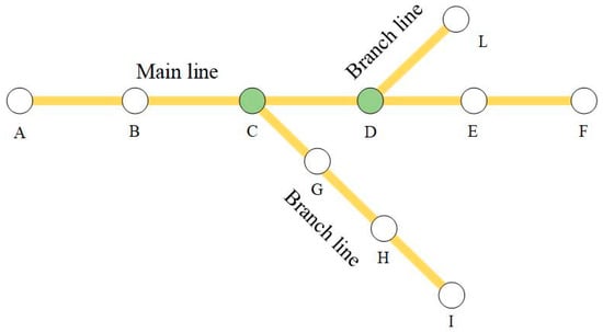
Figure 1.
Plane graph of a railway network.
Figure 2 is a three-dimensional graph that describes the spatiotemporal operation process of the scheduled operation plans. The plane composed of the x-axis and y-axis represents the railway network structure in the real world, and the z-axis represents time. Different colorful lines represent different trains. There are five trains in the figure: Train ① departs from station A to station I, train ② departs from station A to station L, train ③ departs from station A to station F, train ④ departs from station A to station D, and train ⑤ departs from station L to station F. Trains ①, ②, and ⑤ are cross-line trains, and train ③ only departs on the main line. Train ② and train ⑤ are connected by a black line segment, meaning that train ⑤ and train ② share the same train sets.
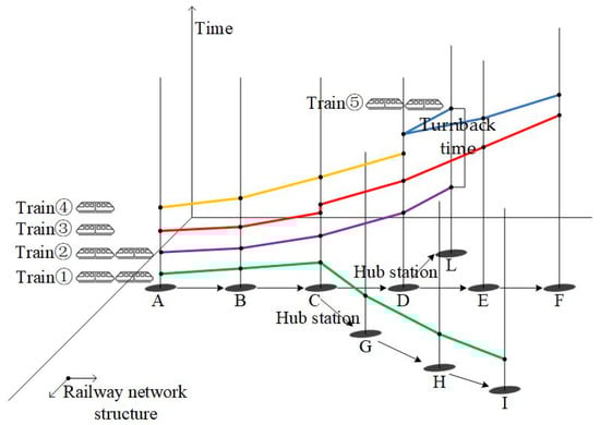
Figure 2.
Spatiotemporal operation process of the scheduled operation plans.
Figure 3 shows some dispatching methods to deal with the influence of emergencies. In this figure, different colorful lines represent different trains. If train ① has an equipment failure when it operates in sections B–C, it will have to stop in the section and wait for rescue. Then, trains ②, ③, and ④ will be delayed for a period of time, as the dash lines show, because they cannot depart from station A until train ①’s rescue operation is finished.
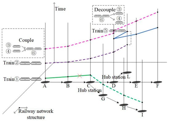
Figure 3.
Spatiotemporal operation process of some dispatching methods after the emergency occurs.
As mentioned above, train ② and train ⑤ share the same train sets. If train ② is delayed for a short period of time, considering the rest turnback time is enough to finish necessary operations, train ⑤ will not be influenced by the delay, as shown in Figure 3. But if train ② is delayed for a long period of time, considering the rest of the connecting time is not enough to finish necessary operations, the operator will have to dispatch a standby train set to undertake the operation plan of train ⑤, or train ⑤ will also be delayed. So, we can see that the train timetable and train set circulation plan are closely related to the rescheduling problems, and it is necessary to reschedule these two aspects together.
Train ③ and train ④ are two delayed short trains. In order to improve operation efficiency, they can be coupled at station A and form a new long train called train ⑥. Train ⑥ operates from station A to station D. And then, train ⑥ is decoupled from train ③ and train ④ at station D.
Besides dispatching standby train sets and coupling short trains, some other methods are also efficient, such as adjusting the arrival time and departure time of the train, changing the sequence of delayed trains, and canceling trains.
Above all, the operators should take all kinds of dispatching methods into consideration when facing an emergency and propose a complete scheme composed of some suitable methods according to the time, location, and other factors of the emergency so as to make the train operation return to normal and reduce the loss of the delay for passengers.
2. Literature Review
In order to deal with emergencies in the process of train operation, researchers have conducted many valuable studies on the rescheduling of train operation plans. For the scope of these studies, some studies focused on a railway line and some studies concentrated on the railway network; for the objects of these studies, some studies mainly focused on train timetable rescheduling, some studies focused on train set circulation plans and a small part of them studied integrated rescheduling methods of train timetable and train sets circulation plan; for the algorithms, many kinds of algorithms are used and they have advantages and disadvantages; and for the optimization objectives, they can be divided into single-objective and multiple-objective.
At the level of the railway line, Meng XL et al. [1] proposed a novel approach to solve the train re-scheduling problem and train control problem synthetically. It also provided supporting information for both the train drivers and the operators to improve the schedule rate and reduce energy consumption. Chung et al. [2] proposed a mixed-integer programming model to balance the operating mileage of bullet trains. They considered the limitation of maintenance capacity and used an improved genetic algorithm to solve the model. Budai et al. [3] proposed a method to reschedule the bullet train operation plan based on the current train timetable. They realized the transition from the old train timetable to the new one. Ghaemi et al. [4] studied a mixed-integer linear programming model for a busy Dutch railway line to obtain the best plan, which includes the station for the train to turn back and the time the train costs. The results show that the plan is related to the length of the emergency period, and a longer period will lead to more train cancellations.
Train operation rescheduling problems on a railway network are also of vital importance. Hu XZ et al. [5] present a mixed-integer nonlinear optimization model of a high-speed railway line planning problem, integrating the operation route plan, train stop plan, and passenger distribution plan. Moreover, a two-stage hybrid heuristic search algorithm is designed to solve this model. Marótiet al. [6] provided a multi-commodity flow model for train timetable adjustment, considering recent train maintenance needs, and tested the model on the Dutch railway network. Pellegrini et al. [7] and Luan et al. [8] proposed a mixed-integer linear programming model to describe the train operation problem and finally solved it with CPLEX. Chen et al. [9] solved the first train scheduling problem to find an optimal scheme by adjusting the total number of skipped stations and the headway of the first deadheading train and tested the method on the Nanjing Railway network.
Train timetable rescheduling plays an important role in the daily operation of the HSR. Thus, some studies mainly focused on train timetable rescheduling under emergency conditions. SchoBel et al. [10] built a mixed-integer linear programming model to make decisions on which trains should be retained in case of train delay. Cacchiani et al. [11] studied the rescheduling of train timetables at the macro level of the railway network. With the objective of minimizing the number of canceled trains and delayed trains, an integer programming model is developed and tested on the Dutch railway network. Wang Zhen [12] established the train operation adjustment model of HSR with the objective function of minimizing the total weighted delay time of the section, and then combined the genetic algorithm and simulated annealing algorithm to solve the model. Gao Xinyu [13] divided the adjustment strategies into two cases when the normal operation status was slightly disturbed and seriously disturbed and used the grey wolf algorithm and the receding horizon algorithm to solve the problem. Gao only considered canceling train services in the case of a serious disturbance. Zhan Shuguang et al. [14] provided an integer linear programming model of real-time adjustment for train operation in view of the serious interruption in high-speed railways in China and designed a two-stage algorithm to get the overall feasible solutions. Then Deng Nian et al. [15] studied the adjustment of train timetables under the condition of a complete interruption of train operation. Samà et al. [16] constructed the train routing selection problem under the condition of emergencies as a mixed-integer programming model. First, they used an ant colony algorithm to solve the feasible route of the train and then adjusted the train timetable based on the obtained feasible route under the condition of emergencies. Finally, they tested the effectiveness of the model and algorithm on the railway lines in France.
Train sets circulation plan is the premise of train timetable execution. Meanwhile, available train sets become scarce in emergency conditions; therefore, a number of studies have focused on train set circulation plans under emergency conditions in order to optimize the plan and save train set resources. Wagenaar et al. [17] proposed a mixed-integer linear programming model to solve the train rescheduling problem, taking into account the dispatching of train sets during emergencies and after the resumption of train operation. Lusby [18] et al. built a model based on the train operation route to optimize the train operation plan during the recovery period caused by an emergency and used a branch and price method to solve the model. Veelenturf et al. [19] established a mixed-integer linear programming model to solve the problem of train timetable rescheduling in the case of a complete interruption. The model can calculate and give the most suitable route, track, and station to turn back. They solved the model by Gurobi and then tested it on two railway lines in the Netherlands.
Some studies considered the train set circulation plan and train timetable together; most of them used a two-stage method, and a few of them explored an integrated adjustment method for the train timetable and train set circulation plan. Based on the feasible train set circulation, Wang Ying et al. [20] used a branch and price method to realize the coordination of the train set circulation plan and train timetable. Different from Wang Ying et al. [20], Wang, ZK et al. [21] integrated the timetable scheduling problem and the rolling stock scheduling problem through a big-M formulation, and the trains are allowed to operate in a platoon according to passenger demand. Cadarso et al. [22] constructed a collaborative adjustment method that can adjust the train operation plan according to passenger demand and then adjust the train timetable and train set circulation plan under emergency conditions. Dollevoet et al. [23] studied the coordination of train timetables and train set circulation plans in the programming stage, and Altazin et al. [24] studied that after emergencies. Compared with the two-stage method, the integrated optimization method can better balance the close coupling relationship between the train timetable and the train set circulation plan and provide more reasonable solutions.
From the perspective of the algorithm, many algorithms are widely applied to solve the rescheduling problem, such as [20] branch and price algorithm, [25] ant colony algorithm, [26] heuristic simulated-annealing algorithm, etc. [1,5]. Both use particle swarm optimization algorithms; the difference is that [1] used particle swarm with quantum-inspired algorithms, and [5] used particle swarm optimization algorithms with genetic algorithm (GA). In recent years, artificial intelligence has been applied to the transportation field. [27] used a random forest algorithm to predict train delays. In order to solve the train rescheduling problem, Kumar [28] used the Brownian motion weighted-based salp swarm optimization (BMW-SSO) algorithm and the modified weight-based deep learning neural network (MWDLNN) algorithm and obtained good results. These algorithms can be applied to a wide range of problem types and domains. They are not limited to specific problem structures or constraints, making them flexible and adaptable in various scenarios. But they also have disadvantages. For example, the branch and price algorithm can be computationally expensive for large-scale problems due to the exponential growth of the solution space; the ant colony algorithm may require a large number of iterations to converge to a good solution; the heuristic simulated-annealing algorithm requires careful tuning of the cooling schedule and acceptance criterion; the particle swarm optimization algorithm may be susceptible to premature convergence, etc.
In 2002, Deb [29] proposed the NSGA-II algorithm to solve two-objective models; based on NSGA-II, Deb [30] proposed the NSGA-III algorithm to solve multi-objective models. The NSGA-III algorithm has been widely studied and applied in various research fields. The NSGA-III algorithm provides a set of diverse solutions that represent the trade-off between different objectives, handles multi-objective optimization problems efficiently without requiring problem decomposition, and enables decision-makers to explore different Pareto optimal solutions and make suitable decisions. It also has disadvantages, such as that the algorithm’s performance heavily depends on the selection of algorithmic parameters, and the computational complexity increases with the number of objectives and the size of the population.
From the perspective of the objectives, some studies used a single objective function model to solve the rescheduling problem after an emergency. Most of them formulated the model with the objective function of train delay. D’Ariano et al. [31] took the minimum total delay time of the train as the objective function and used the branch and bound method to obtain the optimal solution or approximate optimal solution. Lamorgese et al. [32] established a mixed-integer linear programming model with the goal of minimizing the total delay of trains and decomposed the model into two sub-problems by using the master-slave solution algorithm. Hou et al. [33] used the SIS infectivity dynamics model to predict the train delay and took the Wuhan-Guangzhou HSR as an example to study the regularities and the trend of delay propagation within the system. Yuan [34] also used the SIS infectivity dynamics model to predict the train delay, and different from Hou et al. [33], they took the section of Shanhaiguan station to Fuyu North station as an example to test the efficacy of the model. At the level of the railway network, Mu [27] used the random forest model (RF) to predict the delay of trains on the network of the Netherlands, compared the results with the artificial neural network and XGBoost model, and obtained high-precision prediction results. Different from them, Zhu et al. [35] established a mixed-integer linear programming model with the objective of reducing passenger delays and then tested the model on the Dutch railway network. The single objective function is suitable for problems that have just one optimal objective, but for multi-objective problems, it is not applied.
In order to better describe the rescheduling problem, some studies established models with more than one objective. Kroon et al. [6] took the sum of train-related costs and service-related costs as the optimization objective, proposed a train rescheduling model, and finally tested the effectiveness of the model in the busy part of the Dutch railway network. Aimed at improving the punctuality rate of trains, reducing the fluctuation of train operation time in sections, and improving the speed of freight trains, Chen [36] proposed a multi-objective optimization model to synergistically optimize the deviation of the train timetable under disturbance, the energy consumption, and the number of stranded passengers. And the model was further transformed into a linear model to promote problem-solving. Meng [37] took minimizing the generalized punishment of train operation delay and the stability of train operation as the optimization objective functions and defined the satisfaction of the two objective functions for the two-objective programming problem to obtain a feasible solution. Zhang et al. [26] aimed at optimizing both the average deviation of departure intervals and the maximum train loading rate under time-varying passenger transport demand, proposed an optimization model for an irregular train schedule, and designed a heuristic simulated-annealing algorithm to solve the model. Nielsen et al. [38] developed a mixed-integer linear programming model with three objective functions: The penalty value of canceling the train, the penalty value of the scheduling plan, and the penalty value of the deviation between the actual end station and the planned end station. Then they weighted the three objective functions to convert the multi-objective programming into single-objective programming and tested it on a Dutch railway line. A multi-objective function can solve problems with more than one objective and provide a set of diverse solutions for decision-makers. But the computational complexity can be increased compared to a single-objective function.
Above all, we can find that:
- Firstly, many researchers study the rescheduling problem on one railway line; few researchers solve the rescheduling problem on a railway network. While, considering the strong correlations between the railway lines, minor disturbances in the section likely tend to cause larger delays and propagate across the network. Thus, it is of great significance to solve the rescheduling problem on a railway network rather than on one line.
- Secondly, some studies focus on rescheduling train timetables or train set circulation plans, respectively. A small part of the studies uses integrated adjustment methods to deal with the two aspects. However, considering the train set circulation plan supports the feasibility of the train timetable, if emergencies occur, both the train timetable and the train set circulation plan will be deeply influenced. So, it is of great significance to propose an integrated adjustment method for the two aspects when rescheduling.
- Thirdly, in the process of modeling, many studies consider only one objective, such as minimizing train delay, minimizing passenger delay, minimizing the number of canceled trains, etc. Some studies formulate the model with multiple objectives, but most of them use the method of weighting and summing these objectives. While the rescheduling problem is a complex one that involves many factors, it is difficult to describe the problem well with one objective, and the method of weighting and summing objectives is also not appropriate because it is difficult to find a scientific and acknowledged method to determine the weight of objectives.
The main contributions of the paper are as follows:
- In order to deal with the unforeseen events in the HSR network, reduce the propagation of delays on lines and even the whole network, and reduce the influence on passenger travel, we expand our research scope to the network level, which is more challenging and more significant.
- Compared with simply weighing and summing the objectives, we design an algorithm based on NSGA-III to solve the rescheduling problem and obtain a non-dominated Pareto front for three objectives. Each solution in the Pareto Front has a comparative advantage, and the operator can choose a reasonable rescheduling scheme from the front under different circumstances.
- The real-world experiments show that the proposed model and algorithm work well, which can reschedule the train timetable and the train set circulation plan integratedly during an emergency. Moreover, the proposed integrated optimization method can be applied to analyze some characteristics of the network, such as the bottleneck sections of the network, the key time of the whole day, and the importance of the depots.
The remainder of this paper is organized as follows. In Section 3, we formulate an integrated optimization model of the train timetable and train set circulation plan under the condition of HSR network emergencies. In Section 4, we propose an algorithm based on NSGA-III to solve the model. In Section 5, we test our model and algorithm on a busy part of China’s HSR network and obtain a series of feasible solutions for the operators to choose from. And we find out the most critical section and occurrence time and analyze the importance of the depots in the network. Conclusions and future research are discussed in Section 6.
3. Multi-Objective Integrated Optimization Model
In this section, we introduce a multi-objective integrated optimization model to solve the train reschedule problem, which includes the train timetable and train set circulation plan when an emergency occurs. In Section 3.1, we start by explaining the symbols and parameters we use in the model, including sets, symbols, and decision variables. Thereafter, in Section 3.2, we introduce the three objectives of the model, including additional operation cost, total delay, and number of transfer passengers. Finally, in Section 3.3, we explain the constraints of the model, which totals 3 categories and 26 kinds.
The following assumptions are made:
- In order to minimize additional operating costs, if the one train set circulation is not affected, no rescheduling will be made, and only the affected train set circulation will be rescheduled.
- Before the interruption occurs, all trains operate according to the original timetable.
- Only the affected trains and standby train sets can execute the subsequent circulation of the affected trains.
- The standby train sets from different depots can serve all the lines of the railway network.
3.1. Symbols and Parameters
The sets are shown in Table 1, the symbols are shown in Table 2, and the decision variables are shown in Table 3.

Table 1.
Sets.
Table 2.
Symbols.
Table 3.
Decision variables.
3.2. Objectives
- ①
- Minimize additional operation cost
The additional operation mileage at the level of the railway network consists of the running mileage of the standby train sets for subsequent trains in circulation and the mileage back to the allocated station after the completion of the circulation:
is the set of train sets circulations in the railway network, train set circulation . is the set of affected train set circulations. is the set of standby train sets, standby train set . is the set of trains in the railway network, train . is the set of affected trains. Binary variables indicate whether the standby train set executes train of circulation () or not (). is the mileage of standby train set after it completes the circulation that contains train . is the distance between standby train set and its allocated depot after the standby train set completes circulation which contains train . is the operating cost per mileage of standby train set .
- ②
- Minimize total delay
The total delay includes three parts: the delay time of affected passengers who are served by other affected trains; the delay time of passengers who are served by standby train sets; and the delay time of passengers who cannot be served due to train cancellations:
is the set of passenger demands, demand . is the set of affected passenger demands. Binary variables indicate whether the passenger demand of train in circulation is served by train in circulation () or not (). Binary variables indicate whether the train of circulation is cancelled () or not (). Binary variables indicate whether the train in circulation is executed by standby train set () or not (). Decision variables represent the actual arrival time of train in circulation at station after rescheduling. Decision variables mean the actual departure time of standby train set at station after rescheduling. is the passenger number of demand for train in circulation . represents the terminal station of train in circulation . indicates the planned arrival time of train at station in circulation . is the penalty time of cancelling train in circulation .
- ③
- Minimize the transfer number of affected passengers
The transfer number of affected passengers includes two parts: the transfer number of affected passengers served by other affected trains and the transfer number of affected passengers served by standby train sets:
3.3. Constraints
The constraints include 3 types: ① constraints of train timetable, ② constraints of train sets circulation plan, and ③ constraints of passenger demand.
3.3.1. Constraints of Train Timetable
All the trains should meet the constraint of train operation time in the section, as shown in Constraint (4):
And they also should meet the constraint of train operation at the station, as shown in Constraint (5):
In Constraints (4) and (5), is the set of stations in the railway network, station . Decision variables represent actual departure time of train in circulation at station after rescheduling. Binary variables is 1 if train in circulation actually stops at station after rescheduling and 0 otherwise. is the extra departure time of trains at station . is the extra stop time of trains at station . represents the running time of the train in section . is the train stopping time at station .
In the section where the interruption occurs, trains must depart after the interruption has been solved; that is, the departure time of the train should be later than the end time of the interruption, as shown in Constraint (6):
In which, is the end time of the interruption. is the start station of the section where the interruption occurs.
In order to ensure the safety of the trains, the headway time between any two trains should be greater than or equal to the minimum headway time, as shown in Constraint (7).
In Constraint (7), binary variables indicate the sequence of train and train in section , represents that train is in front of train ; otherwise, . is the minimize train delivery headway of two trains. is a sufficiently large numerical value.
Cross-line trains should meet the constraint of station operation time at boundary stations, as shown in Constraint (8):
In which, is the set of cross-line trains. is the set of stations connecting different lines.
If two trains are coupled, they must meet the following Constraints (9)–(16):
The arrival time and the departure time of the two coupled trains are the same at all the stations during the process of coupling, as Constraints (10) and (11) show:
Moreover, the stop stations of the two coupled trains are the same, as shown in Constraint (12):
In addition, the two coupled trains should meet the time constraints at coupled station and the decoupled station, as Constraints (13) and (14) show:
These constraints can be linearized as follows:
In Constraints (9)–(16), represents the set of short trains. are the common sections of train in circulation and train in circulation . Binary variables indicate train in circulation is coupled with train in circulation () or not (). is the operation time of train coupling. is the operation time of train decoupling. is the station where short train in circulation and short train in circulation are coupled. is the station where short train in circulation and short train in circulation are decoupled.
If one train is cancelled, it should meet the following Constraints (17)–(21):
Cancelled trains cannot serve passenger demand, as shown in Constraint (17):
Cancelled trains cannot execute other trains, either, as Constraint (18) shows:
Constraint (19) ensures that cancelled trains cannot be executed:
Moreover, cancelled trains cannot be coupled or decoupled, as Constraint (20) shows:
3.3.2. Constraints of Train Sets Circulation
Constraint (21) expresses that a train can be executed by one train set at most simultaneously:
In which, is the set of train sets in the railway network, train set . Binary variable is 1 if train set executes train of circulation and 0 otherwise.
If a standby train set is operated, it must execute one train, as shown in Constrain (22):
In which, binary variables indicate whether the standby train set is operated () or not ().
Constraint (23) ensures that a standby train set can only execute one train at most simultaneously:
Similarly, a train set can only execute one train at most simultaneously, as shown in Constraint (24):
The affected trains can be executed by other affected trains and standby train sets, or be cancelled, as Constraint (25) shows:
In Constraint (25), binary variables are 1 if train in circulation is executed by train in circulation and 0 otherwise.
Constraint (26) ensures that the train sets and standby train sets must execute all subsequent trains when executing the affected circulation.
Constraint (27) indicates that if the train sets and standby train sets execute the affected trains, the actual departure time of the affected trains cannot be later than the schemed time plus the acceptable maximum associated delay time.
In which, is the set of affected train sets. indicates the serving time of train set at station . is the acceptable maximum associated delay time. is the planned departure time of train at station in circulation .
3.3.3. Constraints of Passenger Demand
We stipulate that the affected passenger demands can be served by affected trains and the standby train sets, while they cannot be served by normal trains.
The number of passengers in each section of the train set or standby train set cannot be more than the seating capacity after serving affected passengers, as Constraint (28) shows.
In constraint (28), indicates whether the passenger demand of train in circulation passes through section , represents that passenger demand passes through section ; otherwise, . is the seating capacity of standby train set . is the seating capacity of train set .
Constraint (29) ensures that the departure time of the train set or standby train set at the station cannot be earlier than the scheduled departure time of the passenger demand it serves.
Constraints (30) and (31) express that if one train serves the passenger demand at one station, the train must stop at that station and must stop at the destination station of the passenger demand.
In Constraints (29)–(31), represents the departure time for passenger demand of train in circulation at station . is the departure station for passenger demand of train in circulation . is the arrival station for passenger demand of train in circulation . is the acceptable maximum coefficient of overcrowding.
The parametric of the model are valued as follows Table 4:
Table 4.
Value of the parametric.
4. NSGA-III Algorithm
Train timetable and train set circulation plan adjustment at the railway network include three objectives. In the real world, the additional operation cost, total delay, and number of transfer passengers are in a constant balance process. If we just take two objectives into account, some better adjustment options will probably be missed, and the quality of the optimization scheme will be influenced, too.
Therefore, in order to improve the quality and diversity of the optimization scheme as much as possible, we use the NSGA-III algorithm, which can take three or more objectives into account at the same time to solve the rescheduling problems. It uses non-dominated sorting to grade individuals in the population, maintains the diversity of the population through well-distributed reference points, and then selects the appropriate population for the next iteration.
4.1. Conception Introduction
4.1.1. Pareto Front
- Dominant relationship
In multi-objective programming, there are dominant relationships and non-dominant relationships. The dominant relationship between the two optimization objectives is described as follows:
In the minimum optimization problem with two objectives, the objective vector is composed of sub-vectors formed by each optimization objective:
For the two decision variables and in the population, there are:
Or:
Then we call dominates , otherwise if there is:
Then we call and do not dominate each other and they are non-dominated.
- 2.
- Pareto rank and Pareto Front
The NSGA-III algorithm classifies the population by calculating how many solutions dominate the current solution. A population may have multiple Pareto levels, as shown in Figure 4:
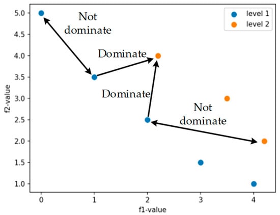
Figure 4.
Pareto level.
As shown in Figure 4, the blue solutions form level 1, and the yellow solutions form level 2. In terms of dominant relationships, the solutions in level 1 do not dominate each other, and the solutions in level 2 do not dominate each other either. But the solutions in level 2 are dominated by some solutions in level 1. At the end of the iteration, the set of solutions with the highest Pareto level constitutes the Pareto front. In this example, level 1 is the Pareto front.
4.1.2. Reference Point Setting
The NSGA-III algorithm is applicable to the problem with a large number of objective functions. In the multi-dimensional space formed by the objectives, the reference point is introduced to preserve the non-dominated individuals in the population that are close to the reference point so as to maintain the diversity of the population.
In order to preserve the diversity of the population, Das and Dennis et al. [39] and Tian Yuan et al. [40] proposed a method to set reference points on the standard plane. They divided each component of the standard plane in the n-dimensional space into P segments and selected reference points on the standard plane at equal intervals. In the optimization problem with M objective functions, the number of reference points () set by this method is:
We take the three-dimensional space with three objectives as an example, as shown in Figure 5:
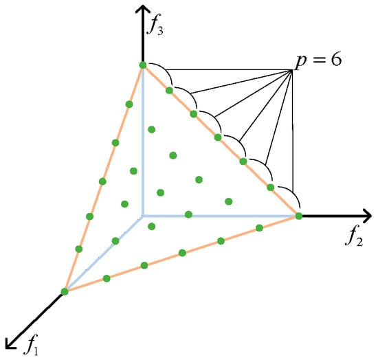
Figure 5.
Reference point generation.
In the multi-objective optimization problem with three objectives (), the yellow triangle is a standard plane, and the analytic representation is:
The coordinates of the reference points meet the following requirements:
After each sub-vector of the standard plane is divided into six segments (), the reference points are shown as the green points in the figure. The number is:
, and the coordinates of the reference points are:
4.1.3. Diversity Determination
After selecting the reference point according to the method in Section 4.1.2, it is necessary to normalize the solution in the Pareto level to be selected so as to avoid the situation where an objective has too much influence on the result due to the difference in the number level of each objective. After normalization, the solutions at the Pareto level are connected with reference points, and the solutions are screened through the connection relationship so as to maintain the diversity of the solutions that enter the next iteration. The connection method between the reference points and the solutions at the Pareto level is shown in Figure 6:
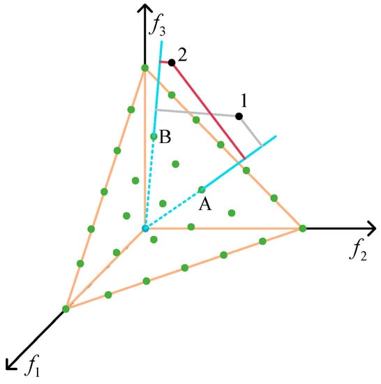
Figure 6.
Reference point selection.
First, the reference point is connected with the origin to form a reference line (blue line). The point at the Pareto level selects the nearest reference line and connects (red lines and grey lines) with the reference point (green points) corresponding to the nearest reference line. As shown in Figure 6, point 1 is closer to reference point A than other reference points, so it is determined that point 1 is connected to reference point A, and point 2 is connected to reference point B.
In the NSGA-III algorithm, diversity is the primary consideration for selecting the individuals for the next generation population, so when we select solutions for the next generation, the individuals of the reference point that have fewer connections can be selected preferentially.
4.2. Representation Scheme
In this algorithm, we represent solutions indirectly by parameters that are later used to obtain a solution by a special decoding procedure. Each chromosome is made of four gene fragments, as Figure 7 shows.
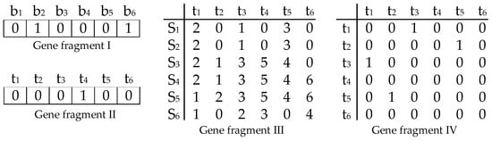
Figure 7.
Gene fragments.
Gene fragment I: The first gene fragment represents the operating scheme of the standby train sets. As shown in Figure 7, − are 6 standby train sets, and number 1 represents the corresponding standby train sets is operated, while number 0 represents the corresponding standby train sets is not operated. Therefore, and are operated, and other standby train sets are not operated.
Gene fragment II: The second gene fragment represents the cancelation scheme of the trains. Number 1 represents the corresponding train is cancelled while number 0 represents not. As shown in Figure 7, − are 6 trains and we can see that is cancelled.
Gene fragment III: The third gene fragment represents the sequence of the trains in the sections. This fragment is a two-dimensional matrix; the abscissa represents trains, and the ordinate represents sections, as shown in Figure 7. Figure 8 is the simple timetable of Figure 7. The colorful lines represent different trains. For example, we can know that the operation sequence of train in section is 4. If one train does not pass through one section, the value will be 0.
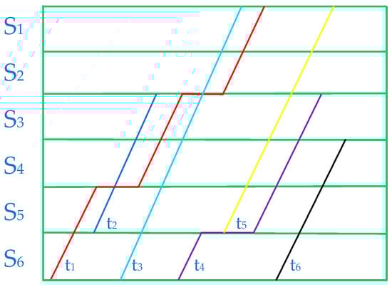
Figure 8.
The simple timetable of gene fragment III.
Gene fragment IV: The last gene fragment represents the coupling scheme of the trains. This fragment is also a two-dimensional matrix; the abscissa and the ordinate both represent trains. Number 1 means the corresponding two trains are coupled, while number 0 means they are not. As shown in Figure 7, and are coupled, while and are coupled, too.
4.3. Initial Populations and Infeasible Solution Adjustment
Gene fragment III is generated according to the original train timetable, while gene fragments I, II, and IV are randomly generated, which may not satisfy the constraints. Therefore, all initial solutions should be checked to obtain a feasible solution set. The infeasible solutions are adjusted as follows:
1. If one train is canceled, it will not be coupled and will not be executed by any train sets, and the sequence value of it in all sections will be 0, as Algorithm 1 shows.
| Algorithm 1: Find the cancelled trains and adjust other gene fragments |
| Step 1. Find the gene fragment I value of train , and let denote it. Find the gene fragment III value of train and section , and let denote it. Find the gene fragment IV value of train and train , and let denote it. Step 2. Create set and add all the to . Create set and add all the to . |
| Step 3. For each train If For each section If Let If Continue For each section If Let If Continue If Continue |
2. If two trains are coupled, they will not be allowed to be coupled with any other trains, as Algorithm 2 shows.
| Algorithm 2: Find the coupled trains and adjust gene fragment IV |
| Step 1. Find the gene fragment I value of train , and let denote it. Find the gene fragment IV value of train and train , and let denote it. Step 2. Create set and add all the to . Create set and add all the to . |
| Step 3. For each train If Continue If For each train If Let the other For each train Let the other If Continue |
3. If two trains are coupled, they will have the same sequence in the sections during the period they are coupled. Therefore, the two trains have the same value of gene fragment IV during the period they are coupled, as shown in Algorithm 3.
| Algorithm 3: Find the coupled trains and adjust gene fragment III |
| Step 1. Find the gene fragment I value of train , and let denote it. Find the gene fragment III value of train and section , and let denote it. Find the gene fragment IV value of train and train , and let denote it. Step 2. Create set and add all the to . Create set and add all the to . Create set . |
| Step 3. For each train If Continue If For each train If Find the same sections and add them to . For each Let If Continue |
4. After the initialization of the solutions, there may be some discontinuous sequence value in a section, such as 0, 1, 3, 4, 5, 0, which should be adjusted to 0, 1, 2, 3, 4, 0. Algorithm 4 shows the process.
| Algorithm 4: Find the discontinuous sequence value adjust gene fragment III |
| Step 1. Find the gene fragment III value of train and section , and let denote it. Step 2. Create set and add all the to . Create set and add all the to . |
| Step 3. Create set . For each section For each train Add to set Find out whether all the nonzero in is continuous, and begin with value 1. If not Adjust all nonzero in to consecutive integers in their original order. If yes Continue |
4.4. Decoding
The chromosomes are made of four gene fragments, which represent the operating scheme of the standby train sets, the cancellation scheme of the trains, the sequence of the trains, and the coupling scheme of the trains, respectively. Thus, the chromosomes have to be decoded to derive the train timetable, the train set circulation plan, and the passenger demand flow plan. Therefore, the decoding process is divided into three main steps.
4.4.1. Calculating and Obtaining Train Timetable
The four gene fragments above can be expressed by the decision variables , , and , respectively (as mentioned in Section 3.1). We stipulation the direction of the interruption direction 1 and the opposite direction is direction 2. We design a sub-model to calculate the timetable of the trains whose direction is direction 1, with the objective of rescheduling the trains of direction 1 in the shortest possible time:
The used sets, symbols and variables are defined in Section 3.1. The model is solved with CPLEX and a group of values of variables. After this part, , , , , , and can be determined.
4.4.2. Rescheduling Train Sets Circulation Plan
After calculating and obtaining the timetable of direction 1-trains, we get the arrival time of these trains at their destination stations. And some train sets of them should continue executing the trains in direction 2 according to their original circulation plan. These trains in direction 2 can be executed by their original train sets, the train sets in other affected circulations, and the standby train sets. The rescheduling algorithm is shown as Algorithm 5:
| Algorithm 5: Rescheduling train sets circulation plan |
| Step 1. Find all the trains of direction 2 which should be executed by train-sets according to the original trains-sets circulation plan. Create set and add them to set . Step 2. For each train Find out whether train can be executed by its original train-set. If yes Train will be executed by its original train-set Remove Train from set . |
| Step 3. Sort the trains according to the departure time at the start station. (from early to late) For each train Find out if train can be executed by the train-sets in other affected circulations. If yes Let the earliest train-sets execute train and remove train from set . Step 4. Sort the trains according to the departure time at the start station. (from early to late) For each train Find out if train can be executed by the standby train-sets. If yes Let the standby train-sets execute train and remove train from set . Step 5. Find out if there are trains in set . If yes Cancel these trains. |
In this part, the variables , , , , and can be determined, and the train-sets circulation plan is rescheduled.
4.4.3. Rescheduling Passenger Demand Flow Plan
In this part, we design a method to reschedule passenger demands. The passenger demands that need to be served consist of the passenger demands of interrupted trains and the passenger demands of canceled trains. The standby train sets and other affected trains can serve these passenger demands. Considering the distance and delay time, this method gives the cross-line passenger demands the priority of being served. The method is shown as follows:
Step 1: Create set , add all the cross-line passenger demands which need be served to . Create set , add all the other passenger demands which need be served to . Create set , add all the standby train-sets to . Create set , add all the other affected trains to .
Step 2: For demand in , judge whether there is train in can serve it. If train can serve demand , three conditions need to be satisfied: (1) The number of passengers cannot be more than the seating capacity of train in any sections. (2) The scheduled departure time of demand should be later than the departure time of train at the start station. (3) train must stop at the departure station and arrival station of demand . If yes, let train serve demand , and remove from set ; if not, go to step 3.
Step 3: Judge whether all the demands in are chosen and judged. If yes, go to step 4; if not, go to step 2.
Step 4: For each demand in , judge whether there is standby train-set in can serve it. If standby train-sets can serve demand , four conditions need to be satisfied: (1) The number of passengers cannot be more than the seating capacity of standby train-set in any sections. (2) The scheduled departure time of demand should be later than the departure time of standby train-set at the start station. (3) standby train-set must stop at the departure station and arrival station of demand . (4) The arrival time of demand plus the servicing time should be earlier than the departure time of the train that standby train-set executed next, so as to make sure the next train can depart at rescheduled time. If yes, let standby train-set serve demand , and remove from set ; if not, go to step 5.
Step 5: Judge whether all the demands in are chosen and judged. If yes, go to step 6; if not, go to step 4.
Step 6: For demand in , judge whether there is train in can serve it. The conditions are the same as that in step 2. If yes, let train serve demand , and remove from set ; if not, go to step 7.
Step 7: Judge whether all the demands in are chosen and judged. If yes, go to step 8; if not, go to step 6.
Step 8: For demand in , judge whether there is standby train-set in can serve it. The conditions are the same as that in step 4. If yes, let train serve demand , and remove from set ; if not, go to step 7.
Step 9: Judge whether all the demands in are chosen and judged. If yes, go to step 10; if not, go to step 8.
Step 10: Cancel the remaining demands in and .
After the process of the method, the variables and are determined till now, all the decision variables mentioned in Section 3.1 are determined.
4.5. Fitness Function
The fitness functions are shown in (41)–(43), which are additional operation cost (), total delay () and the transfer number of affected passengers ().
In every iteration, the Pareto front is generated after calculating these three functions, according to the method in Section 4.1.
4.6. Selection
In order to select superior individuals from the current population and obtain a new population, selection should be performed. First, check the first level of the Pareto front and find out if the number of individuals is less than the population size; if yes, add the first level to the new population and check the next level; otherwise, the progress is as follows, and the definitions are mentioned in Section 4.1.
Step 1: Select the reference point connected to the least number of solution points in the current Pareto level. If there are multiple reference points with the same number of connected solution points, randomly select one reference point from them.
Step 2: Determine the number of solution points in the current Pareto level that the reference point is connected to. If the reference point is not connected to other solution points, reselect the reference point. If the reference point is connected to solution points in the Pareto level, go to Step 3.
Step 3: Judge whether there are connected points higher than the current Pareto level that have entered the next iteration. If there are solution points meeting the requirements, it indicates that the diversity of the current reference point has been preserved. Randomly select a point to enter the next iteration. If there are no solution points meeting the requirements, it indicates that the diversity of the current reference point needs to be preserved. Then, select the solution point closest to the reference line corresponding to the current reference point and add it to the next iteration. Go to Step 4.
Step 4: Judge whether the population size of the next iteration meets the population size. If not, go to Step 1. If yes, end the selection process.
Till now, we have obtained a new population.
4.7. Crossover
Crossover is one of the genetic operations that combines two chromosomes to generate a new chromosome. We use to describe the probability of one chromosome which is chosen to cross with another chromosome. In Section 4.4, different Pareto levels are formed, and we assume that there are Pareto levels in total. can be obtained by following formulas.
is the number of individuals in the -th Pareto level, is the probability of choosing a chromosome to cross from the -th Pareto level. can be obtained by following formulas.
If there is only one Pareto level, then:
is the number of the population size.
We choose a crossover point randomly for the crossover progress of the four gene fragments, respectively. After that, we get some new chromosomes, and we should ensure the infeasibility of these solutions. Therefore, we use the adjustment strategy proposed in Section 4.2 to ensure the feasibility of these new solutions.
4.8. Mutation
The mutation is another operation in the process of generating new chromosomes. The mutation probability of each fragment is 15%.
As for gene fragment I and gene fragment II, we randomly choose a gene and change the value. Since the variables of gene fragment I and gene fragment II are 0–1 variables, the result of mutation is the value of the selected gene changing from 0 to 1 or from 1 to 0.
As for gene fragment III, we randomly select two adjacent trains and exchange their sequence from one section by making the train behind overtake the other train. And we renew the corresponding values in the matrix of the two trains.
As for gene fragment IV, we randomly select two coupled trains and decouple them. The corresponding values in the matrix of the two trains should be changed from 1 to 0. Then, we randomly select two short trains and couple them. The corresponding values in the matrix of the two trains should be changed from 0 to 1.
4.9. Termination Conditions
The algorithm ends and outputs the result when there are no new individuals being added to the Pareto front for continuous 30 iterations or when the number of iterations reaches the predetermined value.
4.10. Algorithm
The framework of the algorithmic procedure is summarized as follows in Figure 9.
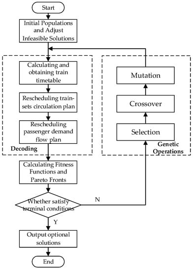
Figure 9.
Flow chart of the solution approach.
5. Case Study
In this section, we set up a series of experiments to test our model and algorithm. All the computational tests are performed by an Intel (R) Xeon (R) processor with 32 cores and 64 GB RAM.
5.1. Basic Data
We use a whole day’s train timetable, ticket selling data, and train set circulation plan of a Chinese railway network as the basic data. All the input data above is from our team’s engineering project. The railway network structure is shown in Figure 10 as follows. It is composed of Beijing–Shanghai HSR (BS Line, the red line), Tianjin–Qinhuangdao HSR (TQ Line, the yellow line), and Tianjin–Baoding HSR (TB Line, the blue line). BS Line starts from BJS station and ends at SHHQ station, with a total of 23 stations; TQ Line starts from TJW station and ends at QHD station, totaling 9 stations; TB Line starts from TJW station and ends at BD station, totaling 7 stations.
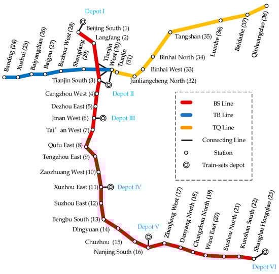
Figure 10.
Railway network structure.
The basic data for the three lines are shown in Table 4:
There are 6 train set depots in the network, and Table 5 shows the service scope of the depots.
Table 5.
Basic data of the three lines.
The CZ depot serves all three lines, and the operator can dispatch standby train sets from the depot to the TB Line and TQ Line by TJX railway station or to the BS Line by TJN railway station. The other 5 depots serve the BS Line and TQ Line.
5.2. Adaptability Analysis of NSGA-III Algorithm
We set a one-direction interruption from station 19 to station 18, which starts at 9:00 am. and lasts for 90 min. We use the algorithm in Section 4 with 30 population sizes and 1000 iterations, and the solving time is 2673 s. The comparison before and after iteration is plotted in Figure 11.
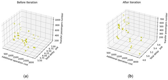
Figure 11.
Comparison before and after iteration. (a) The solutions before iteration; (b) The solutions after iteration.
As Figure 11 shows, the left part is the 30 solutions before iteration, and the right part is the result of the 30 solutions after iteration. The detailed comparison of them is shown in Table 6.
Table 6.
Service scope of the depots.
We can see that the average value of all three objectives declines to different degrees, which are 14.12%, 12.12%, and 10.57%, respectively, indicating that our algorithm can improve the quality of the individuals effectively.
In order to test and verify the effectiveness of our model and algorithm, we collected the values of three objectives (additional costs, total delay, and transfer number of affected passengers) for 1000 generations and plotted three convergence curves based on these values. The convergence curves are as follows:
In Figure 12, we can see that all three objectives reach a relatively stable value during the iteration, which indicates the effectiveness of our model and algorithm.
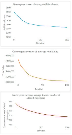
Figure 12.
Convergence curves.
Then, we run our optimization algorithm 10 times and obtain 10 groups of average objectives after optimization. We calculated the mean value, the standard deviation, and the coefficient of variation, as Table 7 and Table 8 shows.
Table 7.
Detail comparison before and after iteration.
Table 8.
The mean value, the standard deviation, and the coefficient of variation.
We can find that the 10 optimization results have no significant difference; the standard deviation is 3.86, 1787.01, and 4.76, respectively, and the coefficient of variation is 2.82%, 0.35%, and 0.95%, respectively. The small standard deviation and coefficient of variation indicate that our algorithm has considerable reliability and reproducibility.
While, the mean computation time of the method is 2691.20 s, which is a relatively long period of time. We consider that the long period of time is due to the large scale of the rescheduling problem, which is the disadvantage and limitation of the method. However, the coefficient of variation is 3.0%, indicating a certain degree of stability for the method.
5.3. Analyze the Bottleneck Section and Key Time
There are a total of 36 sections in the railway network. Generally speaking, if an emergency occurs in different railway sections, it will have different influences on the railway network. Similarly, the emergency occurring at different times also has different influences on the network. Therefore, we try to test the different occasions in order to analyze the characteristics of the network.
We designed a group of experiments as follows. For each section, we set 6 one-direction interruptions starting at 9:00, 11:00, 13:00, 15:00, 17:00, and 19:00, respectively, and the duration is 90 mins. Then, we run our algorithm 216(36 × 6) times and obtain a Pareto front at each time. For each of the 216 Pareto fronts, we calculate the average of the total delay, respectively, obtain 216 three-dimensional points (X (railway section), Y (occurrence time), Z (total delay)), and fit a three-dimensional figure with these points as follows.
In Figure 13, the left part shows the optimization result of the BS Line, and the right part shows the optimization results of the TQ Line and the TB Line.
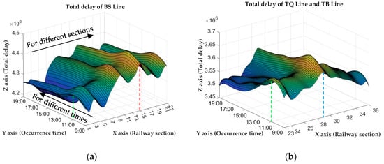
Figure 13.
The total delay of three lines after optimization. (a) The total delay of BS Line after optimization. (b) The total delay of TQ Line and TB Line after optimization.
5.3.1. Bottleneck Section
In the left part of Figure 13, from the X-axis (railway section) point of view, section 15 has the maximum total delay for any interruption occurrence time, indicated by the red dashed line. Therefore, we can call section 15 the bottleneck section of the whole network. It means that if one interruption occurs in section 15, it will have a more significant influence than any other sections on the total delay of the railway network, which should be paid more attention by the operator.
We think the reason is that, from the data of the train timetable, there are most trains operated in section 15 and many of them are cross-line trains. So, if one interruption occurs in section 15, many trains will be influenced, and the delay of these trains will propagate through the railway network, and then, the total delay of the whole network will increase greatly.
We also find that in the right part of Figure 13, for each occurrence time, the total delay of section 29 is obviously greater than other sections, as the blue dashed line indicates. We think the reason is that section 29 is located at the junction of the TB Line and TQ Line, and there are more trains (especially cross-line trains) operated in section 29 than in other sections of the two lines. If the cross-line trains are delayed, it will directly influence more lines and sections, and the propagation of delays will be more significant. Therefore, section 29 should also be given more attention by the operator.
Above all, we can find that the operators should pay more attention to the sections in which most trains operate or are located at the junction of the network. Because they are likely to become bottleneck sections.
5.3.2. Key Time
From the Y-axis (occurrence time) point of view, the total delay of 11:00 is always the highest for any section, as indicated by the green dashed line in Figure 13. So, we can call 11:00 the bottleneck time. It means that if the interruption occurs at this time, the interruption will have a greater influence on the network and the total delay will have a significant increase, which should be given more attention during the operation.
We think the reason is similar to the above; from the data of the train timetable, most trains operate on the network around 11:00. In addition, this period is popular for passengers, and the average number of passengers on each train is high. If one interruption occurs at this time, more trains and passengers will be influenced and delayed, and the total delay will be high.
5.4. Analysis of the Importance of the Depots
In order to analyze the importance of the depots, we assume that each depot has unlimited standby train sets for emergencies and design a series of experiments as follows. We set a one-direction interruption in each of the 36 sections, respectively. All 36 interruptions start at 9:00 am. and last for 180 min.
For each interruption, we run our algorithm and get a Pareto front with a group of solution points. For each front, the sum of the standby train sets dispatched from each depot is calculated, and the depot dispatching the most standby train sets is called the “key depot” of the interruption. For all the interruptions, 36 Pareto fronts are obtained, and the times of each depot being a key depot are calculated and plotted in Figure 14.
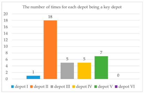
Figure 14.
The number of times for each depot being a key depot.
We can see that depot II becomes a key depot 18 times, which is the most. So, we can say that, compared with other depots, depot II plays a significantly important role in this railway network. It means that if the number of train sets in all depots is unlimited and the probability of interruption occurring in each section is equal, dispatching standby train sets from depot II is the most efficient. In other words, the operation department should deploy more standby train sets in depot II.
We think the reason is that depots I, III, IV, V, and VI are located on the BS Line and mainly serve the BS Line. Depot II is located in the center of the railway network and has a wider service scope, as mentioned in Section 5.1. For most of the sections, depot II can provide rescue with less additional cost because of its location and connection to the network.
6. Conclusions
In the event of emergencies occurring in the HSR network, we proposed a multi-objective model with the objectives of additional operation cost, total delay, and the number of transfer passengers. We designed an algorithm based on NSGA-III to solve the model. Rather than simply weighting and summing the three objectives, the algorithm optimizes the objectives together and provides a Pareto front with a group of non-dominated solutions for operators to choose from. We tested the adaptability of the proposed model and algorithm on a real-world railway network in China. After 1000 iterations, we obtained a Pareto front containing a group of feasible solutions for the operators to choose from in different situations. We compared the average value of the three objectives in these solutions before and after optimization and obtained the optimization rate, which is 12.12%, 14.12, and 10.57%, respectively, indicating that our method can improve the quality of the solutions effectively. We also run the algorithm 10 times and calculate the mean value, the standard deviation, and the coefficient of variation of the objectives. The coefficients of variation are 2.82%, 0.35%, and 0.95%, respectively, which indicates that our algorithm has considerable reliability and reproducibility.
We also proposed an integrated optimization method to reschedule the train timetable and the train set circulation plan at the network level. The proposed method combines different dispatching methods in the model and reschedules the above two plans integratedly rather than rescheduling them in stages. Moreover, we designed a group of experiments with one-direction interruptions that occur in different sections and at different times. Then, we analyzed the total delay and discovered the bottleneck section (section 15) and the bottleneck time (11:00). Finally, we set up a series of cases to analyze the importance of the depots. By counting the number of times that the depot is a key depot, we give the operator some advice to set more standby train sets in depot II when formulating the train set layout scheme and conclude that depot II is more important than other depots in the network.
We assume the probability of interruption occurring in each section is equal when we analyze the importance of the depots. However, the occurrence of emergencies has certain regularities. If future research conducts an in-depth study of the regularities, the analysis and suggestions for the deployment of the standby train sets will be more convincing and significant.
Author Contributions
Conceptualization, W.Z., L.Z. and B.G.; methodology, W.Z., B.G. and Y.Y.; software, W.Z. and Z.W.; validation, W.Z. and B.G.; formal analysis, W.Z. and Y.M.; investigation, W.Z., B.G. and C.H.; resources, W.Z. and Y.M.; data curation, W.Z.; writing—original draft preparation, W.Z.; writing—review and editing, L.Z., B.G. and Y.Y.; visualization W.Z., C.H. and Y.M.; supervision, L.Z. and B.G.; project administration, W.Z., B.G. and Y.Y., funding acquisition, B.G. and Z.W. All authors have read and agreed to the published version of the manuscript.
Funding
This research was funded by Research Supported by the Fundamental Research Funds for the Central Universities (Science and technology leading talent team project), grant number 2022JBQY005; Research project of China State Railway Group Co., Ltd., grant number K2021X002; and Research project of China Railway Beijing Group Co., Ltd., grant number 2022BY02.
Institutional Review Board Statement
Not applicable.
Informed Consent Statement
Not applicable.
Data Availability Statement
Not applicable.
Acknowledgments
The authors would like to express great appreciation to editors and reviewers for their positive and constructive comments. And thanks are due to Hanxiao Zhou for data curation and funding acquisition.
Conflicts of Interest
The authors declare no conflict of interest.
References
- Meng, X.L.; Wang, Y.H.; Lin, L.; Li, L.; Jia, L.M. An Integrated Model of Train Re-Scheduling and Control for High-Speed Railway. Sustainability 2021, 13, 11933. [Google Scholar] [CrossRef]
- Chung, J.; Oh, S.; Choi, I. A hybrid genetic algorithm for train sequencing in the Korean railway. Omega 2009, 37, 555–565. [Google Scholar] [CrossRef]
- Budai, G.; Maróti, G.; Dekker, R.; Huisman, D.; Kroon, L. Rescheduling in passenger railways: The rolling stock rebalancing problem. J. Sched. 2009, 13, 281–297. [Google Scholar] [CrossRef]
- Ghaemi, N.; Cats, O.; Goverde, R.M.P. Macroscopic multiple-station short-turning model in case of complete railway blockages. Transp. Res. Part C Emerg. Technol. 2018, 89, 113–132. [Google Scholar] [CrossRef]
- Hu, X.Z.; Wang, H.W.; Wu, X.T.; Zhou, M.; Dong, H.R. An Integrated Optimization Approach of High-Speed Railway Line Plan to Network Load-Balancing; Chinese Automation Congress (CAC): Shanghai, China, 2020. [Google Scholar]
- Kroon, L.; Maroti, G.; Nielsen, L. Rescheduling of Railway Rolling Stock with Dynamic Passenger Flows. Transp. Sci. 2015, 49, 165–184. [Google Scholar] [CrossRef]
- Pellegrini, P.; Marlière, G.; Rodriguez, J. Optimal train routing and scheduling for managing traffic perturbations in complex junctions. Transp. Res. Part B Methodol. 2014, 59, 58–80. [Google Scholar] [CrossRef]
- Luan, X.; Corman, F.; Meng, L. Non-discriminatory train dispatching in a rail transport market with multiple competing and collaborative train operating companies. Transp. Res. Part C Emerg. Technol. 2017, 80, 148–174. [Google Scholar] [CrossRef]
- Chen, Y.Z.; Shi, C.L.; Hu, M.B. Energy-Efficient Scheduling of the First Train with Deadheading in Urban Railway Networks. IEEE Access 2022, 10, 113061–113072. [Google Scholar] [CrossRef]
- Schöbel, A. A Model for the Delay Management Problem based on Mixed-Integer-Programming. Electron. Notes Theor. Comput. Sci. 2001, 50, 1–10. [Google Scholar] [CrossRef]
- Veelenturf, L.; Kidd, M.; Cacchiani, V.; Kroon, L.; Toth, P. A Railway Timetable Rescheduling Approach for Handling Large-Scale Disruptions. Transp. Sci. 2016, 50, 841–862. [Google Scholar] [CrossRef]
- Wang, Z. Study on Operation Adjustment of High-Speed Trains Based on Genetic Simulated Annealing Algorithm. Master’s Thesis, Beijingjiaotong University, Beijing, China, 2019. [Google Scholar]
- Gao, X. Models and Algorithms for High-Speed Train Rescheduling in Typical Disrupted Scenarios. Master’s Thesis, Beijingjiaotong University, Beijing, China, 2020. [Google Scholar]
- Zhan, S.; Zhao, J.; Peng, Q.; Xu, P.; Zhang, X. Real-time Train Rescheduling on High-speed Railway under Complete Segment Blockage. J. China Railw. Soc. 2015, 37, 1–9. [Google Scholar]
- Deng, N.; Peng, Q.; Zhan, S. Real-time Train Rescheduling on High-speed Railway under Disruption Condition. J. Transp. Syst. Eng. Inf. Technol. 2017, 17, 118–123. [Google Scholar]
- Samà, M.; Pellegrini, P.; D’Ariano, A.; Rodriguez, J.; Pacciarelli, D. Ant colony optimization for the real-time train routing selection problem. Transp. Res. Part B Methodol. 2016, 85, 89–108. [Google Scholar] [CrossRef]
- Wagenaar, J.; Kroon, L.; Fragkos, I. Rolling stock rescheduling in passenger railway transportation using dead-heading trips and adjusted passenger demand. Transp. Res. Part B Methodol. 2017, 101, 140–161. [Google Scholar] [CrossRef]
- Lusby, R.M.; Haahr, J.T.; Larsen, J.; Pisinger, D. A Branch-and-Price algorithm for railway rolling stock rescheduling. Transp. Res. Part B Methodol. 2017, 99, 228–250. [Google Scholar] [CrossRef]
- Veelenturf, L.P.; Kroon, L.G.; Maróti, G. Passenger oriented railway disruption management by adapting timetables and rolling stock schedules. Transp. Res. Part C Emerg. Technol. 2017, 80, 133–147. [Google Scholar] [CrossRef]
- Wang, Y.; Liu, J.; Miao, J. Optimization of the Circulation Plan for Multiple Unites Based on Adjustable Train Path. China Railw. Sci. 2012, 33, 112–119. [Google Scholar]
- Wang, Z.K.; Su, B.Y. Integrated train timetable and rolling stock circulation plan scheduling with the virtual coupling technology for a Y-shaped metro line. In Proceedings of the IEEE International Conference on Intelligent Transportation Systems-ITSC, Macau, China, 12 August 2022. [Google Scholar]
- Cadarso, L.; Marín, Á.; Maróti, G. Recovery of disruptions in rapid transit networks. Transp. Res. Part E Logist. Transp. Rev. 2013, 53, 15–33. [Google Scholar] [CrossRef]
- Dollevoet, T.; Huisman, D.; Kroon, L.G.; Veelenturf, L.P.; Wagenaar, J.C. Application of an iterative framework for real-time railway rescheduling. Comput. Oper. Res. 2017, 78, 203–217. [Google Scholar] [CrossRef]
- Altazin, E.; Dauzère-Pérès, S.; Ramond, F.; Tréfond, S. Rescheduling through stop-skipping in dense railway systems. Transp. Res. Part C Emerg. Technol. 2017, 79, 73–84. [Google Scholar] [CrossRef]
- Eaton, J.; Yang, S.X.; Mavrovouniotis, M. Ant colony optimization with immigrants schemes for the dynamic railway junction rescheduling problem with multiple delays. Soft Comput. 2016, 20, 2951–2966. [Google Scholar] [CrossRef]
- Zhang, H.; Ni, S.Q. Train Scheduling Optimization for an Urban Rail Transit Line: A Simulated-Annealing Algorithm Using a Large Neighborhood Search Metaheuristic. J. Adv. Transp. 2022, 2022, 9604362. [Google Scholar] [CrossRef]
- Mu, W. Study on the Train Prediction Model by Using the Real Operation Data of the Dutch Railway Network. Master’s Thesis, Southwest Jiaotong University, Chengdu, China, 2017. [Google Scholar]
- Kumar, N.; Mishra, A. An efficient method of disturbance analysis and train rescheduling using MWDLNN and BMW-SSO algorithms. Soft Comput. 2021, 25, 12031–12041. [Google Scholar] [CrossRef]
- Deb, K.; Pratap, A.; Agarwal, S.; Meyarivan, T. A fast and elitist multi-objective genetic algorithm: NSGA-II. IEEE Trans. Evol. Comput. 2002, 6, 182–197. [Google Scholar] [CrossRef]
- Deb, K.; Jain, H. An Evolutionary Many-Objective Optimization Algorithm Using Reference-Point-Based Nondominated Sorting Approach, Part I: Solving Problems With Box Constraints. Evol. Comput. 2014, 18, 577–601. [Google Scholar] [CrossRef]
- D’Ariano, A.; Pacciarelli, D.; Pranzo, M. A branch and bound algorithm for scheduling trains in a railway network. Eur. J. Oper. Res. 2007, 183, 643–657. [Google Scholar] [CrossRef]
- Lamorgese, L.; Mannino, C. An Exact Decomposition Approach for the Real-Time Train Dispatching Problem. Oper. Res. 2015, 63, 48–64. [Google Scholar] [CrossRef]
- Hou, Y.; Jiang, C.; Li, L.; Huang, P. SIS Epidemic Model for Delay Propagation of High-speed Train. China Transp. Rev. 2019, 41, 48–53+69. [Google Scholar]
- Yuan, Q. Research on Delay Distribution and Propagation Model of High-Speed Train. Master’s Thesis, Beijingjiaotong University, Beijing, China, 2020. [Google Scholar]
- Zhu, Y.; Goverde, R.M.P. Railway timetable rescheduling with flexible stopping and flexible short-turning during disruptions. Transp. Res. Part B Methodol. 2019, 123, 149–181. [Google Scholar] [CrossRef]
- Chen, C.; Zhu, L.; Wang, X. An Integrated Train Scheduling Optimization Approach for Virtual Coupling Trains. In Proceedings of the IEEE 25th International Conference on Intelligent Transportation Systems (ITSC), Macau, China, 12 August 2022. [Google Scholar]
- Meng, X. Theories and Methods on Train Operating in Emergency. Ph.D. Thesis, Beijingjiaotong University, Beijing, China, 2011. [Google Scholar]
- Nielsen, L.K.; Kroon, L.; Maróti, G. A rolling horizon approach for disruption management of railway rolling stock. Eur. J. Oper. Res. 2012, 220, 496–509. [Google Scholar] [CrossRef]
- Das, I.; Dennis, J. Normal-boundary intersection: A new method for generating the Pareto surface in nonlinear multicriteria optimization problems. Siam J. Oper. 1998, 8, 631–657. [Google Scholar] [CrossRef]
- Tian, Y.; Xiang, X.S.; Zhang, X.Y.; Cheng, R.; Jin, Y.C. Sampling Reference Points on the Pareto Fronts of Benchmark Multi-Objective Optimization Problems. In Proceedings of the IEEE Congress on Evolutionary Computation (IEEE CEC) as part of the IEEE World Congress on Computational Intelligence (IEEE WCCI), Rio de Janeiro, Brazil, 13 August 2018. [Google Scholar]
Disclaimer/Publisher’s Note: The statements, opinions and data contained in all publications are solely those of the individual author(s) and contributor(s) and not of MDPI and/or the editor(s). MDPI and/or the editor(s) disclaim responsibility for any injury to people or property resulting from any ideas, methods, instructions or products referred to in the content. |
© 2023 by the authors. Licensee MDPI, Basel, Switzerland. This article is an open access article distributed under the terms and conditions of the Creative Commons Attribution (CC BY) license (https://creativecommons.org/licenses/by/4.0/).