Article

100 Picosecond/Sub-10−17 Level GPS Differential Precise Time and Frequency Transfer

1
School of Electronic and Information Engineering, Beihang University, Beijing 100083, China
2
Key Laboratory of Navigation and Communication Fusion Technology, Ministry of Industry and Information Technology, Beijing 100083, China
3
Research Institute for Frontier Science, Beihang University, Beijing 100083, China
*
Author to whom correspondence should be addressed.
Appl. Sci. 2023, 13(19), 10694; https://doi.org/10.3390/app131910694
Submission received: 24 August 2023 / Revised: 19 September 2023 / Accepted: 25 September 2023 / Published: 26 September 2023

Abstract

:
A Global Navigation Satellite System (GNSS) is a high-precision method for comparing clocks and time transfer. The GNSS carrier phase can provide more precise observable information than pseudorange. However, the carrier phase is ambiguous, and only pseudorange can provide the absolute time difference between two clocks. In our study, by taking full advantage of GNSS pseudorange and carrier-phase observables, a differential precise time transfer (DPT) method with a clustering constraint was employed to estimate the time difference between two clocks, aiming to achieve accurate and precise time and frequency transfer. Using this method, several time transfer results were analyzed for different baselines. For the common clock experiment, the time transfer results showed good consistency across different days, with an intra-day accuracy of within 20 ps. Furthermore, we evaluated the self-consistency of DPT using closure among three stations. DPT closure of the three stations had a peak-to-peak value of closure of about 25 ps. The closure did not change over time, indicating the self-consistency of the DPT processing in time transfer. Moreover, our results were compared to station clock solutions provided by the International GNSS Service (IGS), and the standard deviations (STDs) of the four baselines were all less than 100 ps within one month, confirming the time and frequency stability of the DPT method. In addition, we found that the time stability of DPT was less than 20 ps within one week. As for frequency stability, DPT achieved a 10−16 level of modified Allan deviation (MDEV) at an averaging time of about 1 day and a sub-10−17 level at an averaging time of one week.

1. Introduction

Time transfer technology is a prerequisite for time synchronization and timing, and high-precision time and frequency transfer technology is particularly important for achieving high-precision time and frequency services. Since the early 1980s, time and frequency transfer based on Global Navigation Satellite Systems (GNSSs) has been widely developed. Satellite one-way time dissemination, as the simplest GNSS time transfer method, provides clock solutions with an accuracy of 20–30 nanoseconds [1]. The Satellite Common View (CV) method provides a relatively high accuracy in short-baseline time comparisons [2]. However, the distance and accuracy of time transfer are limited by the availability of common satellites and the target range measurement [3,4]. In 2004, Jiang et al. [5] proposed the All-in-View (AV) satellite time transfer method as an improvement over the CV method. With AV, time transfer distance is no longer limited by the availability of common satellites [6,7]. However, both methods use pseudorange, and the pseudorange multipath and noise limit the time and frequency transfer performance, such that only nanosecond-level time transfer can be achieved [8].
Considering that GNSS carrier-phase measurements are two orders of magnitude more accurate than pseudorange measurements, it is possible to further improve time transfer performance by using phase measurements. Schildknecht et al. [9] first used GPS carrier-phase measurements to validate high-precision time and frequency transfer. As a continuation of the AV method, the Precise Point Positioning (PPP) method uses both pseudorange and carrier-phase measurements for high-precision un-difference time and frequency transfer, and it has been widely promoted in the time community, becoming the main means used by the Bureau International des Poids et Mesures (BIPM) for comparing clocks contributing to International Atomic Time (TAI) techniques [10,11,12]. In addition, using carrier-phase differential methods for high-precision time and frequency transfer has become a complementary method. In 2007, J. Delporte et al. [13] directly fixed the single-difference (SD) integer ambiguity by combining AV and CV technology with SD pseudorange and carrier-phase measurements, realizing SD carrier-phase time transfer. This method is suitable for post-processing analysis. In 2008, Lee et al. [14] utilized International GNSS Service (IGS) orbit and clock products to calculate carrier-phase AV and carrier-phase CV clock solutions and realized GPS carrier-phase CV and AV time transfer. In addition, the method based on real-time kinematics (RTK) double difference has also been used to recover high-precision inter-station clock information. Feng et al. [1] proposed a four-dimensional real-time kinematics (4D-RTK) timing method, which further recovered the inter-station SD integer carrier-phase ambiguity based on double-difference observations to obtain relative clock solutions and achieved a precision of better than 0.1 ns on a 21 km baseline for a duration of 1.5 h. What is more, Tu et al. [3] further compared the time difference estimates obtained from the RTK and PPP methods using short baseline links; the STD of the time difference between the two methods was about 0.1 ns. However, while using the carrier phase to improve the precision of clock comparison, the accuracy of time transfer is often overlooked.
If the primary focus is on time transfer rather than frequency transfer, the issue of an absolute time difference in carrier-phase time transfer solutions also needs to be solved. Since the carrier phase is ambiguous, only pseudorange can provide the absolute time difference between two stations, so the method using only the carrier phase can only provide frequency transfer results. In order to provide accurate time difference results between two stations, it is necessary to introduce pseudorange to determine receiver clock offset in carrier-phase time transfer. However, as it is affected by the noise and multipath of pseudorange, it is difficult to fix the SD integer ambiguity.
For the problem of integer ambiguity resolution, Teunissen et al. [15] proposed a least-squares ambiguity decorrelation adjustment (LAMBDA) method based on integer Gaussian transformation in 1995. Since then, the LAMBDA method has been widely used for DD integer ambiguity resolution in RTK positioning [16,17,18]. In 1999, Teunissen et al. [19] further summarized integer rounding, integer bootstrapping, and integer least squares for a class of integer estimators and demonstrated the best performance of the integer least-squares estimator.
In this study, the LAMBDA method was used for the determination of double-difference (DD) ambiguities. When estimating SD ambiguities from pseudorange measurements, we employed the integer rounding estimator based on the K-means algorithm to determine their integer values and then achieved differential precise time and frequency transfer (DPT). To verify the performance of DPT, common clock time transfer experiments were analyzed and calibrated, as well as three stations’ closure time transfer results. In addition, we evaluated time and frequency transfer performances for four baselines over 30 days. The discussion and conclusion are given in the final section.

2. Differential Precise Time and Frequency Transfer

The key problem to be solved by the differential precise time and frequency transfer of GNSS is to obtain high-precision inter-station clock offset. First, based on the GNSS observations of the time reference station and the user station, the DD mathematical model is established, and the solution of DD carrier-phase ambiguities and the corresponding variance matrix are obtained. Secondly, the reference satellite is selected to calculate the receiver clock offset through the SD pseudorange observation, then the inter-station SD carrier-phase ambiguity of the reference satellite is estimated, and, further, the inter-station SD carrier-phase ambiguities of all visible satellites are estimated. Affected by pseudorange noise and multipath, there may be a bias in the estimation of SD carrier-phase ambiguity by the integer rounding estimator. Then, we determine the final SD integer carrier-phase ambiguities by the K-means clustering method [20,21]. Once the ambiguities are determined, the carrier phase can provide the “absolute” time difference between stations. Finally, the accurate time transfer based on the SD carrier-phase observation is realized. In the following, the detailed DPT method will be introduced.

2.1. Double-Difference Fixed Ambiguity Resolution

In the field of geodesy, the mathematical model for relative positioning [22] based on DD pseudorange and the carrier phase for frequency, f , is expressed as:
P f ( m , n ) i , j = ρ f ( m , n ) i , j + e p h f ( m , n ) i , j + T f ( m , n ) i , j + I f ( m , n ) i , j + ε P f ( m , n ) i , j L f ( m , n ) i , j = ρ f ( m , n ) i , j + e p h f ( m , n ) i , j + T f ( m , n ) i , j I f ( m , n ) i , j + λ f N f ( m , n ) i , j + ε L f ( m , n ) i , j
where P f ( m , n ) i , j and L f ( m , n ) i , j represent DD pseudorange and carrier-phase observations from satellites i and j to receivers m and n, respectively. ρ f ( m , n ) i , j represents the DD geometric distance, e p h f ( m , n ) i , j represents the DD ephemeris error residual, T f ( m , n ) i , j represents the DD tropospheric delay residual, I f ( m , n ) i , j represents the DD ionospheric delay residual, N f ( m , n ) i , j represents the DD carrier-phase integer ambiguity, and λ f is the corresponding wavelength. ε P f ( m , n ) i , j and ε P f ( m , n ) i , j are the sum of the multipath errors and measurement noise of the DD pseudorange and carrier-phase observations, respectively.
For relative positioning technology, when the distance between two receivers is a short baseline of up to a few kilometers, the DD tropospheric and ionospheric delay residuals can be ignored [23]. The LAMBDA method [16] is used to determine the DD integer carrier-phase ambiguity. In addition, the dual-frequency ionosphere-free (IF) combination can also be used to eliminate the impact of the first-order term of ionospheric delay for longer baselines. DD wide-lane integer ambiguities, N W m , n   i , j , between two stations are calculated by using the Melbourne–Wübbena combination observation and then obtaining the float DD carrier-phase ambiguity, N I F m , n i , j , of the IF combination.
N I F m , n i , j = 1 λ 1 · f 1 2 f 1 2 f 2 2 · λ 1 · N f 1 m , n i , j f 2 2 f 1 2 f 2 2 · λ 2 · N f 2 m , n i , j = f 1 f 1 + f 2 N f 1 m , n i , j + f 1 · f 2 f 1 2 f 2 2 N W m , n i , j
where N W m , n i , j = N f 1 m , n i , j N f 2 m , n i , j . The DD carrier-phase ambiguity of the IF combination can be estimated from IF combination observation. Furthermore, L1 DD integer ambiguity, N f 1 m , n i , j , can be obtained.
N f 1 m , n i , j = f 1 + f 2 f 1 N I F m , n i , j f 2 f 1 f 2 N W m , n i , j
where · denotes rounding to the nearest integer.

2.2. Single-Difference Ambiguity Estimation

According to Equation (1), it is known that the DD carrier-phase ambiguity solution eliminates the receiver clock offset, which is the most crucial parameter in time and frequency transfer. To retain the clock offset, we perform inter-station SD resolution using the pseudorange and carrier-phase observations. The SD model is shown in Equation (4):
P f ( m , n ) i = ρ f ( m , n ) i + c · t r f ( m , n ) j + e p h f ( m , n ) i + T f ( m , n ) i + I f ( m , n ) i + ε P f ( m , n ) i L f ( m , n ) i = ρ f ( m , n ) i + c · t r f ( m , n ) j + e p h f ( m , n ) i + T f ( m , n ) i I f ( m , n ) i + λ f N f ( m , n ) i + ε L f ( m , n ) i
where t r f ( m , n ) j represents the inter-station SD receiver clock offset and c represents the speed of light. For the SD carrier-phase observation, receiver clock offset and SD carrier-phase ambiguity are linearly dependent. To separate them, we introduce the initial value of the inter-station receiver clock offset through SD pseudorange observation and then obtain SD carrier-phase ambiguity. When DD carrier-phase ambiguities are fixed, we use the pseudorange and carrier-phase observations to calculate the float SD carrier-phase ambiguity, N f ( m , n ) i ( t ) , at epoch t . For short baselines of several kilometers, ignoring the SD ionospheric delay residual, the SD tropospheric delay residual, and the SD ephemeris residual, Equation (5) can be obtained:
N f m , n i ( t ) = 1 λ f ( L f m , n i ( t ) P f m , n i ( t ) )
Due to the influence of the noise and multipath of pseudorange, it is generally difficult to accurately determine the SD integer ambiguity using only one epoch of pseudorange measurement. It is known that the ambiguity remains continuous for each visible satellite once the receiver is correctly locked. Therefore, we smoothed Equation (5) for l epochs to reduce the effects of pseudorange noise and multipath and obtained the float SD carrier-phase ambiguity, which is shown in Equation (6). Usually, the pseudorange noise and multipath of the satellite at the highest elevation is the smallest, so the reference satellite can be selected by using the satellite elevations.
N ¯ f ( m , n ) i = 1 l t = 1 t = l N f m , n i ( t ) = 1 l λ f t = 1 t = l ( L f m , n i ( t ) P f m , n i ( t ) )
When using Equation (6) to determine the SD integer ambiguity, the number of epochs required is closely related to the precision of pseudorange measurement. It is generally believed that integer ambiguity can be determined when the accuracy of the average value reaches ±6 cm [24]. Then, we use the integer rounding method to obtain the SD integer carrier-phase ambiguity, N f ( m , n ) i , of the reference satellite, i , as shown in Equation (7).
N f ( m , n ) i = N ¯ f ( m , n ) i = 1 l λ f t = 1 t = l ( L f m , n i ( t ) P f m , n i ( t ) )
where · denotes rounding to the nearest integer. After obtaining the fixed DD integer ambiguity by Equation (1) and the SD integer ambiguity of reference satellite i by Equation (7), it is easy to obtain SD integer ambiguity, N f ( m , n ) j , of the visible satellite, j , by using Equation (8).
N f ( m , n ) j = N f ( m , n ) i + N f ( m , n ) i , j
After obtaining L1 DD integer ambiguity and DD wide-lane integer ambiguities, N W m , n i , j , by using Equations (2) and (3), IF combination SD ambiguity, N I F m , n j , of the visible satellite, j , can be obtained.
N I F m , n j = N I F m , n i + N I F m , n i , j = N I F ( m , n ) i + f 1 f 1 + f 2 N f 1 m , n i , j + f 1 · f 2 f 1 2 f 2 2 N W m , n i , j
From Equation (6), it can be found that estimating the SD carrier-phase ambiguity of the reference satellite, i , requires a convergence time. When the precision of pseudorange measurement of P codes is about ±0.3 m, the determination of the ambiguity requires about 25 epochs of pseudorange observations [24]. If the epoch number,   l , is reduced, the determination of SD carrier-phase ambiguity is inevitably affected by the pseudorange noise and multipath. Next, the pseudorange noise and multipath affect the time transfer performance.
In the double-difference positioning solution, it is a common practice to select the satellite with the maximum elevation as the reference satellite. However, when solving the single-difference ambiguity of the reference satellite using Equation (3), it is inevitable that the influence of the pseudorange noise and multipath will be present. To further reduce the impact of the pseudorange noise and multipath on the SD integer ambiguities, we take each visible satellite as a reference satellite separately and estimate the SD integer ambiguities.
As soon as a set of SD integer ambiguity samplings is available, we can classify them into groups according to their distribution. This group is also called a cluster, a region in which the density of samples is locally higher than in other regions [25]. In this contribution, the K-means clustering method is employed to determine SD integer ambiguities. The K-means algorithm aims to choose the best clusters that minimize the sum square error of the distances between a sample and its cluster centroid [25]. The problem can be expressed mathematically as:
P ( S S 1 ,   , S n ) = m i n i = 1 n j = 1 m   x i j μ i 2 μ i = 1 m j = 1 m x i j       i = 1 ,   , n
where S is the set of total samples and S 1 ,   , S n is the set of n clusters from S 1 to S n . For each cluster, S i , there are m samples, x i j is the j th sample of the i th cluster, and μ i is the centroid of the i th cluster.
In this study, the clustering is applied on SD integer ambiguities, and we set the initial groups according to satellite PRN. For each group, its centroids, μ i , from all members, x i j , are calculated using Equation (10). In practice, the solving process of K-means is an optimization problem. In this study, we selected the cluster with the most data sampling points as the final SD integer ambiguity.

2.3. Time Difference Estimation of DPT

In order to obtain the time difference solution between two stations, we introduce the SD integer ambiguities into SD carrier-phase measurements, achieving accurate time transfer. For a short baseline of several kilometers, the inter-station receiver clock offset is shown in Equation (11) after ignoring the SD ephemeris error residuals, tropospheric delay residuals, and ionospheric delay residuals.
t r f ( m , n ) = 1 c L f ( m , n ) j ρ f ( m , n ) j λ f N f ( m , n ) j
For the IF combination, the receiver clock offset is shown in Equation (12).
t r I F ( m , n ) = 1 c L I F ( m , n ) j ρ I F m , n j λ I F N I F m , n j T I F m , n j
where t r f ( m , n ) represents the f frequency DPT time transfer result and t r I F ( m , n ) represents the IF combination DPT time transfer result.

3. Experiment Strategy

To explicitly investigate and analyze the performance of the time and frequency transfer solutions with the proposed DPT method, eight baselines composed of IGS stations were selected. The detailed information of the eight baselines is presented in Table 1. Using the GPS calibration results provided by BIPM as a reference, the time transfer results for the USN7-USN8 baseline verify the accuracy of DPT time transfer. For the baseline closure consisting of the three short baselines NYA1-NYA2, NYA2-NYAL, and NYAL-NYA1, it verifies the self-consistency of DPT time transfer. In evaluating the long-term time and frequency performance of the baselines, four sets of baselines with external atomic clocks, namely, KOKV-KOVB, CEBR-VILL, KOUR-KOUG, and ONSA-SPT0, are used to verify the DPT time and frequency stability. Table 2 summarizes the information about the data and settings in the DPT data processing.

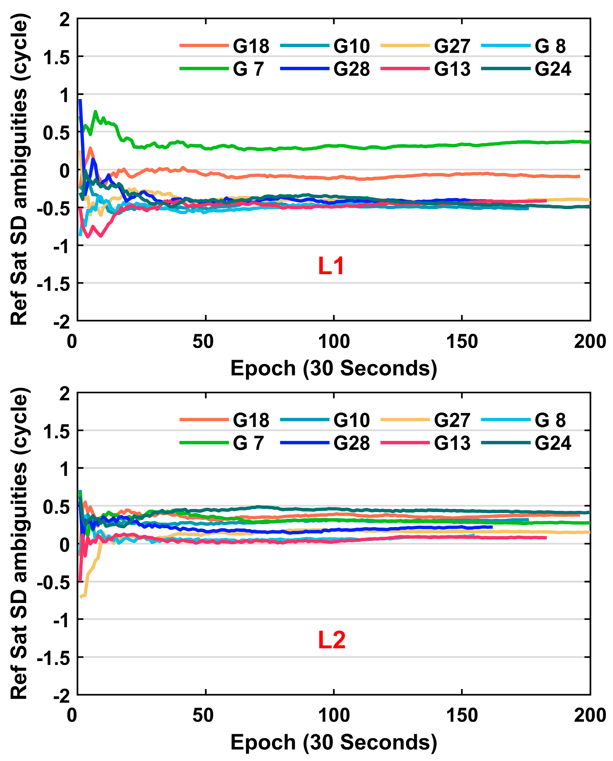
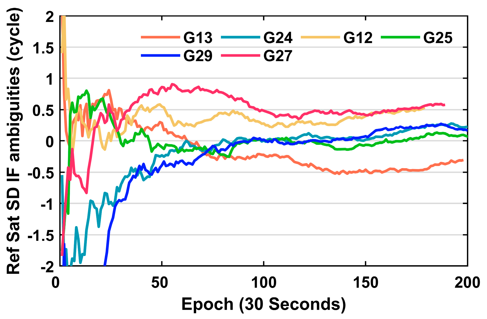
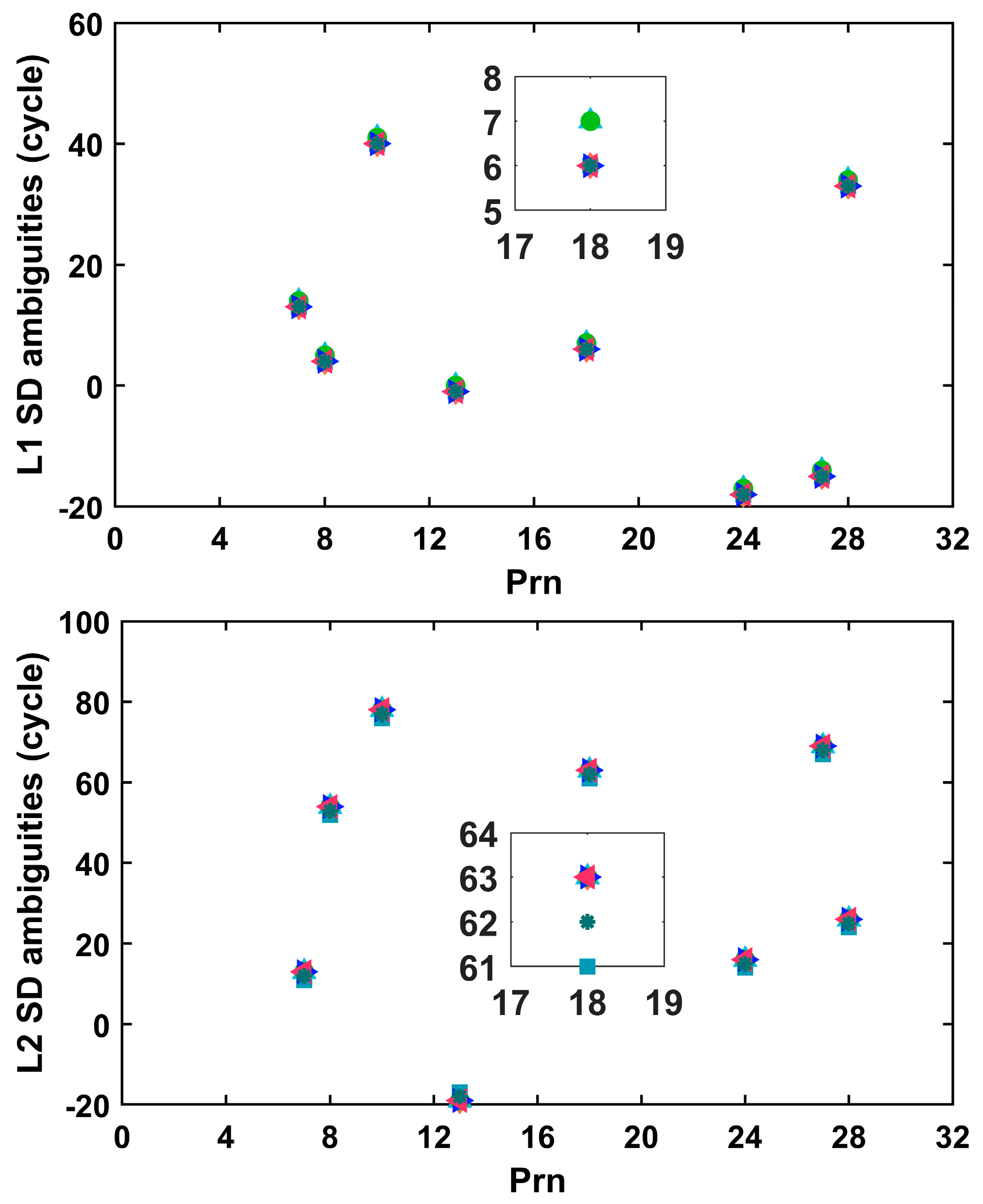
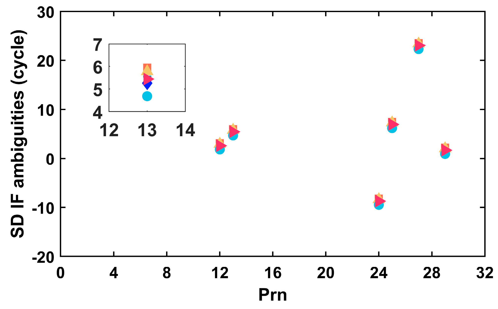
4. Single-Difference Ambiguity Analysis

The float SD carrier-phase ambiguity of the reference satellite can be obtained by using Equation (3). We took each visible satellite as a reference satellite separately and estimated the L1 and L2 SD ambiguities of the reference satellites. For the KOKV-KOVB baseline, the fractional part of the SD ambiguity of the reference satellite is shown in Figure 1. Note that KOKV-KOVB is the zero baseline. For the baseline of ONSA-SPT0 with a length of 67 km, the fractional part of the reference satellite SD ambiguity is shown in Figure 2. It is believed that when the peak-to-peak value of the SD carrier-phase ambiguity fractional part time series is less than 1/3 cycles and it remains stable in subsequent epochs, the integer ambiguity can be determined.
As shown in the upper panel of Figure 1, the L1 SD carrier-phase ambiguities of eight visible satellites were obtained using the L1 carrier phase and the C1 code in MJD 59,764. It can be clearly seen that within 25 epochs (12.5 min for 30 s simple intervals), the peak-to-peak values of the L1 SD carrier-phase ambiguity fractional parts time series are less than 1/3 cycles, and the converged carrier-phase ambiguities remain stable in subsequent epochs. The bottom panel of Figure 1 plots the SD carrier-phase ambiguities obtained using the L2 carrier phase and the P2 code and shows the convergence of the solutions. It took 8 min to reduce the peak-to-peak values of the L2 SD carrier-phase ambiguity fractional parts time series to less than 1/3 cycles. In addition, for the ONSA-SPT0 baseline in Figure 2, it can be observed that the IF SD carrier-phase ambiguities for each visible satellite were resolved within 40 min.
After determining the SD integer ambiguity of the reference satellite and the DD integer ambiguity, we used each visible satellite as a reference satellite to obtain the SD integer ambiguity of the other visible satellites by Equation (6). Figure 3 plots the L1 and L2 SD ambiguities of G07, G08, G10, G13, G18, G24, G27, and G28 for KOKV-KOVB. It is known that the ambiguity of each visible satellite remains continuous as long as the carrier-phase observation is continuously observed. It can be observed that the estimated SD ambiguities differ depending on the reference satellite used. Taking G18 as an example, when using five different satellites as a reference, the estimated L1 SD ambiguities were 6. However, when using the other two different satellites as a reference respectively, the L1 SD ambiguities were estimated to be 7. Similarly, for the L2 SD ambiguities, when using five different satellites as a reference respectively, the estimated values were 63; when using the other one satellite as a reference, the L1 SD ambiguity was estimated to be 62; and using the rest of the satellites as a reference, the L1 SD ambiguity was estimated to be 61. It can be concluded that there are differences in SD ambiguity resolution using different reference satellites, which affects the accuracy of the time difference solution obtained by Equations (10) and (11). Clustering the results of these SD carrier-phase ambiguities, it can be determined that the L1 SD ambiguity is 6 and the L2 SD ambiguity is 63 for G18.
For the ONSA-SPT0 baseline, Figure 4 illustrates the GPS IF combination SD carrier-phase ambiguities of G12, G13, G24, G25, G27, and G29. Taking G13 as an example, it can be observed that the IF SD carrier-phase ambiguities for each visible satellite are different, and it is not the integer number of cycles because IF combined observations cause the ambiguity to lose integer properties. After clustering the results of these SD carrier-phase ambiguities, the final IF SD ambiguity of G13 was determined to be 5.6.

5. DPT Time and Frequency Transfer Validations

In this section, we first verified the accuracy of time transfer through two methods: common clock time transfer and DPT with closure baseline. Then, we evaluated the precision of long-term DPT time transfer through 30 days of continuous solutions. Finally, we analyzed the time and frequency stability of DPT.

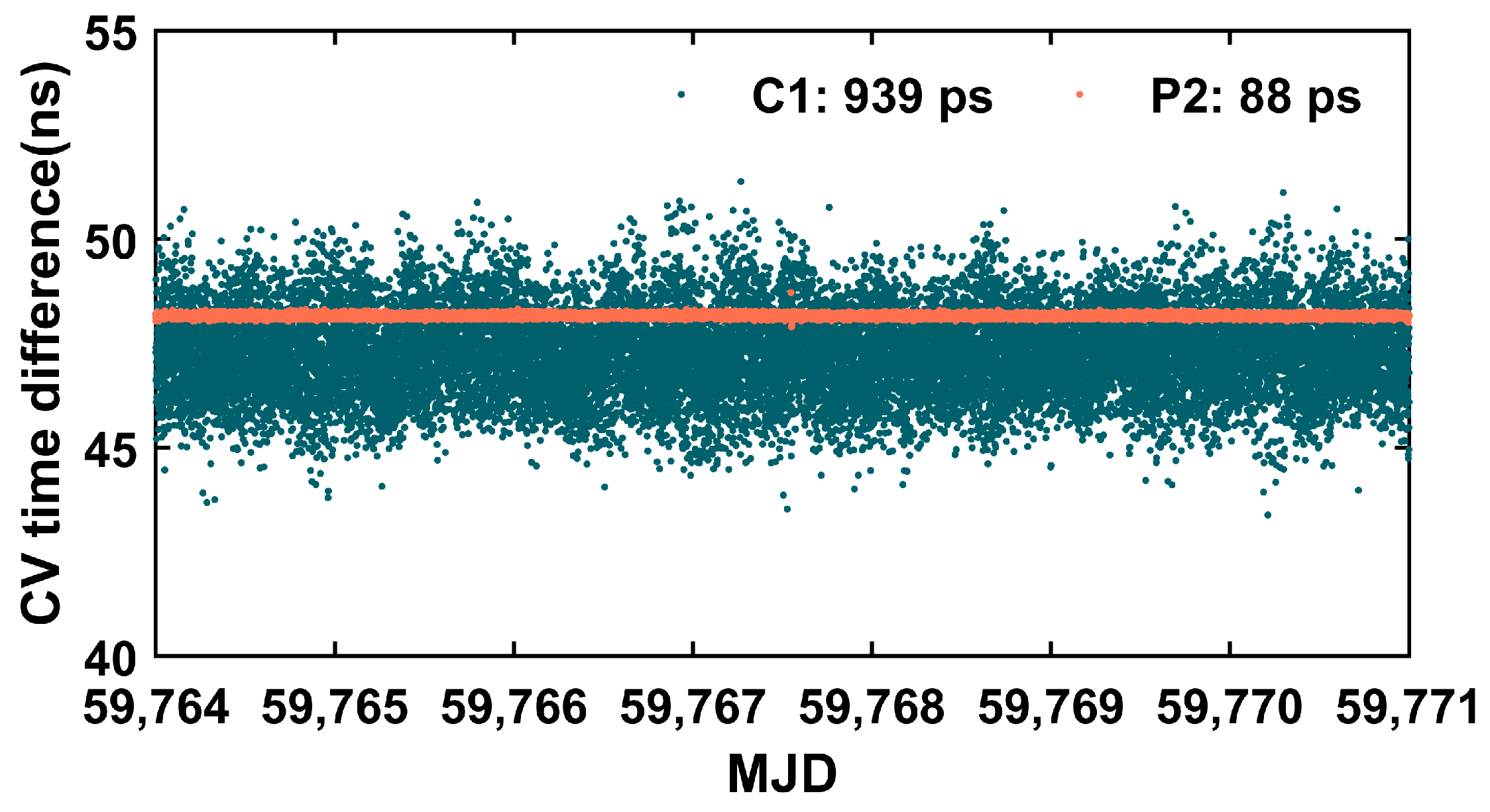
5.1. DPT Time Transfer in a Common Clock

Data from two independent receivers, USN7 and USN8, are being operated at the United States Naval Observatory (USNO) in Washington, DC, using a common reference clock that is regularly calibrated using GPS time transfer. As the time transfer solution of the two stations is expected to constant and known, it is relatively easy to evaluate the expected results of DPT.
To verify the accuracy of the DPT time difference, we conducted time transfer experiments on the USN7 and USN8 stations and performed daily re-initialization. We collected 7 days’ CV time transfer results during MJD 59,764.0–59,770.0, as shown in Figure 5. For the estimated time difference over these 7 days, the standard deviation (STD) for the C1 code was 939 ps and for the P2 code it was 88 ps. As expected, it is well known that the precision of the P code is ten times that of the C1 code due to its narrower code chip width. Since the initial value of DPT time transfer depends on pseudorange time transfer, the accuracy of CV time transfer for different codes will affect DPT time transfer.
The DPT time transfer results are shown in Figure 6. Note that the results have been calibrated using the calibration results published by BIPM, as shown in Table 3, by subtracting the time delays associated with the stations CAB, REF, and INT, along with their respective uncertainties [26]. The calculation is as follows:
t ( f ) = t ( f ) T O T ( f ) U S N 7 T O T f U S N 8 0
where f represents the L1 frequency or L2 frequency, t ( f ) represents the DPT solution, and T O T f represents the total time delay of a geodetic system for frequency f, which is divided into six different parts, including antenna delay, antenna cable delay, receiver internal delay, short cable and splitter delay, internal reference delay, and 1 PPS delay [27].
For the time difference solutions estimated for 7 days in Figure 6, the STD and mean results of the GPS DPT and CV time transfer daily solutions after convergence are shown in Table 4. The STDs of the converged time difference for the GPS L1 and L2 frequencies were 18 ps and 4 ps, respectively. As expected, due to the heavy noise level in the C1 code, time transfer relying on the C1 code requires a long time to converge, making it difficult to determine the absolute time for DPT with high precision. Meanwhile, the estimated time difference solutions for the 7 days had mean convergence values of 291 ps for GPS L1 frequency and 70 ps for the GPS L2 frequency. As a time transfer experiment, the time difference solution between the USN7 and USN8 stations should be zero in theory, and the closure of the two stations shows the accuracy of the DPT time transfer. In Figure 6, there is a constant difference of about 300 ps using the C1 code. This difference may be due to uncertainties of DPT solution or the calibration uncertainties from BIPM, or the combination of DPT and the calibration. Furthermore, we validate the time transfer of DPT through closure experiments in the next sub-section.

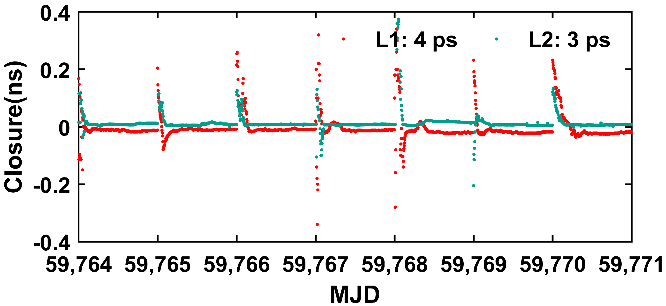
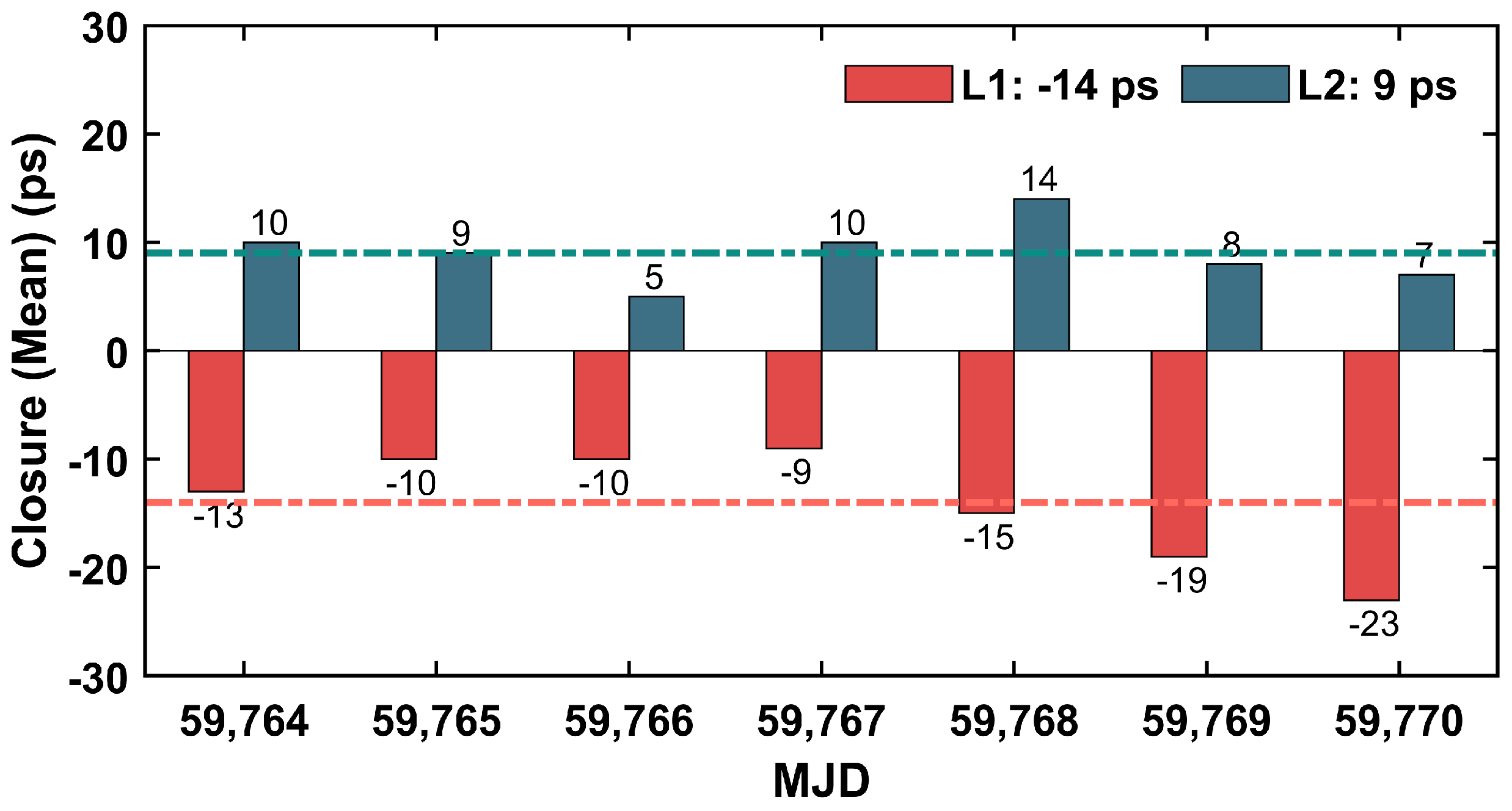
5.2. DPT Time Transfer Validations with Closure Baselines

In order to further verify the accuracy of the DPT time difference, we determined the time transfer between each of the NYA1, NYA2, and NYAL stations and performed daily re-initialization for 7 days. We further evaluated the self-consistency of the DPT using the three stations’ closure in Figure 7. Theoretically, the three stations’ baseline closure is given by:
Closure = ( N Y A 1 N Y A 2 ) + ( N Y A 2 N Y A L ) + ( N Y A L N Y A 1 ) = 0
As shown in Figure 7, the estimated closure solutions for the 7 days had STD values of 4 ps for the GPS L1 frequency and 3 ps for the GPS L2 frequency after the initialization. Meanwhile, Figure 8 shows the mean value of the baseline closure of the daily solutions. The two dashed lines in Figure 8 represent the average values over 7 days for GPS L1 and L2 frequencies, with the GPS L1 frequency at −14 ps and the GPS L2 frequency at 9 ps after initialization. Notably, the closure did not change over time, indicating that the DPT processing is self-consistent in terms of time transfer. This consistency reinforces the reliability of the DPT technique for accurate time transfer.

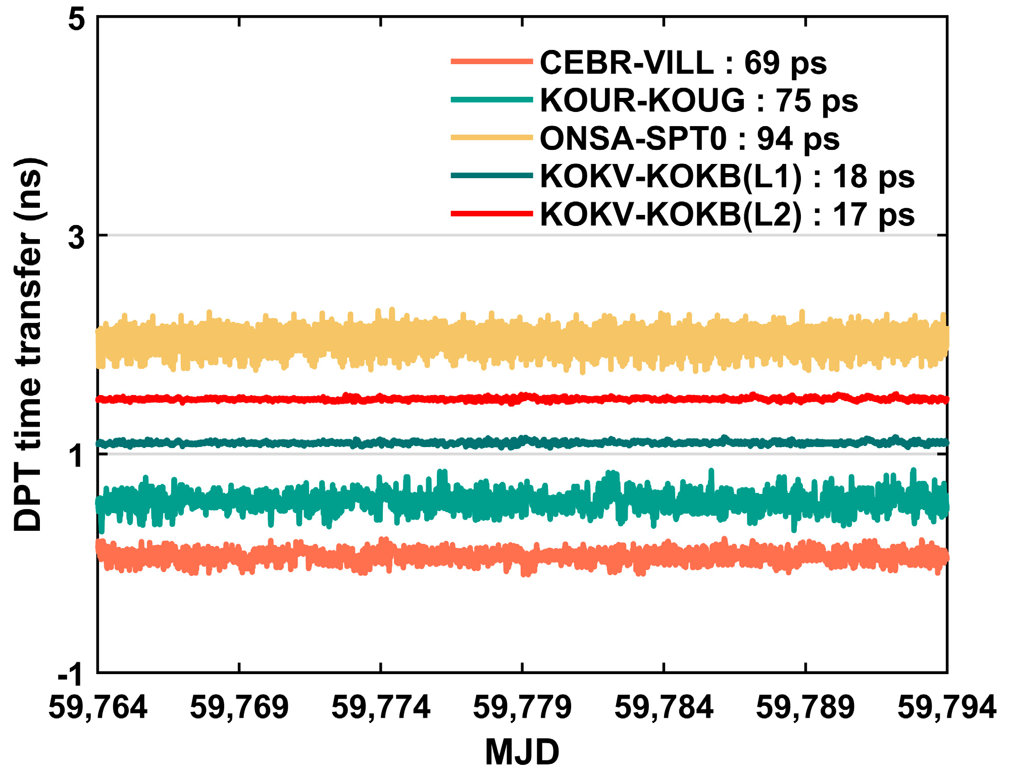
5.3. Long-Term DPT Time and Frequency Transfer Validations

We analyzed the common clock experiment between USN7 and USN8 and the three stations’ baseline closure test and verified that DPT can accurately determine the initial value of DPT time transfer. In addition, we also selected four baselines, CEBR-VILL, ONSA-SPT0, KOUR-KOUG, and KOKV-KOVB, for continuous time transfer and further considered the long-term performance of DPT. Table 1 presents the details of the four baselines. To remove the trend effects of the time difference between two station clocks, a common reference time is introduced to subtract the inconsistency between the two clocks. Typically, IGS final station clock solutions are used as the reference times due to their precision of 20 ps (STD) [28]. The data sampling rate of the IGS final station clock solutions is 5 min. In order to better compare with the reference, the time difference solution of DPT is also set with a sampling interval of 300 s. The result of DPT is then:
T i m e   t r a n s f e r = ( T A T B ) ( I G S T A I G S T B )
Figure 9 displays the time differences between different L1 and L2 frequencies and the dual-frequency IF combination DPT for four different baselines. It should be noted that none of the four baselines were calibrated and that a constant offset was added to each curve for comparison. It can be seen that the time difference estimated by the five curves shows the same trend. Among them, the KOKV-KOKB baseline was processed using single-frequency L1 or L2 time transfer, with STDs of 18 ps (the L1 frequency for KOKV-KOKB (L1)) and 17 ps (the L2 frequency for KOKV-KOKB (L2)) over a period of 30 days. The reason why the time difference results of the DPT time transfer are so flat is that the initial value of DPT time transfer depends on pseudorange time transfer, and after this initial value is determined, only the carrier phase is used, so the noise in the code is well eliminated. As the baseline distance between the reference station and the user station increases, the DD atmospheric delay cannot be ignored. Therefore, the CEBR-VILL, KOUR-KOUG, and ONSA-SPT0 baselines were processed using the dual-frequency IF combination, with STDs of 69, 75, and 94 ps, respectively. Compared with single-frequency processing, the IF combination used here amplifies the noise to a certain extent, especially for the ONSA-SPT0 baseline shown in Figure 9.
From the above, we analyzed the long-term time transfer performance of DPT of four baselines, CEBR-VILL, ONSA-SPT0, KOUR-KOUG, and KOKV-KOVB. For the evaluation of frequency stability, compared with Allan deviation, modified Allan deviation (MDEV) has the advantage of distinguishing white and flickering phase modulation noise and is often used for frequency stability evaluation [29]. In addition, time deviation (TDEV) is used to characterize the time stability of time links [30]. In this work, we used TDEV and MDEV to analyze the time and frequency stability of DPT, respectively, which were obtained using the Stable32 software [31]. Smaller MDEV and TDEV values indicate better time and frequency stability.
Figure 10 and Figure 11 show the stability results of MDEV and TDEV for the four baselines. As shown in Figure 10, the single frequency DPT has an MDEV of 9 × 10⁻¹⁷ at an averaging time of 1 day and 3 × 10⁻¹⁸ at an averaging time of 7 days. The IF DPT has an MDEV of 3 × 10⁻¹⁶ at an averaging time of 1 day and 2 × 10⁻¹⁷ at an averaging time of 7 days. Figure 11 shows that the time stability of the IF DPT is less than 20 ps for an averaging time of 1 day, especially less than 10 ps within 7 days. As for the single-frequency DPT, the time stability is less than 4 ps for an averaging time of 1 day and approaches 1 ps within 7 days.

6. Discussion

Compared with some existing results of GNSS pseudorange time and frequency transfer techniques, such as CV and AV, DPT indeed improves the time and frequency stability and thus enhances the performance of frequency comparison over averaging times of several hours or longer. In addition, a K-means clustering method was employed to estimate the SD receiver clock offset, which achieves accurate time transfer. The time stability can reach the picosecond level on the averaging time of 7 days, while the frequency stability can reach the sub-10−17 level. Among the existing GNSS time and frequency transfer methods, integer PPP (IPPP) has been proven to have the best clock comparison performance [32,33], and the common clock IPPP approach has achieved a time transfer precision of 61 ps, which is comparatively less precise than DPT time transfer in the KOKB-KOKV baseline. In terms of frequency stability, the MDEV of the common clock IPPP experiment over a 30-day period is no less than 1 × 10⁻¹⁷, while the MDEV of the DPT frequency transfer for the KOKB-KOKV baseline can reach as low as 3 × 10⁻¹⁸ within 30 days. To our knowledge, these results represent the optimal proven time transfer precision and frequency stability performance of GNSS time and frequency transfer.
As expected, for short baselines, single-frequency DPT provides higher precision than dual-frequency IF DPT, and the dual-frequency IF combination amplifies noise to some extent. Therefore, for short baselines, we can prioritize the use of single-frequency DPT for time and frequency comparison. The use of the DPT method is complementary to the PPP time transfer method and can achieve high-precision regional time transfer. It only uses broadcast ephemeris to achieve high-precision time transfer and is easier to implement in real-time dynamic applications. In addition, the excellent frequency stability of DPT frequency transfer helps to evaluate the frequency comparison performance in the region of the latest-generation optical lattice clock frequency standard. It should be noted that this work did not discuss longer baselines. For longer baselines, we will consider incorporating precise ephemeris in future research to improve time transfer accuracy.

7. Conclusions

In this paper, a differential precise time transfer (DPT) with a clustering constraint method was employed to estimate the time difference between two clocks, aiming to achieve accurate and precise time and frequency transfer. For the experiment of common clock time transfer, the DPT time transfer results showed good consistency across different days, with an intra-day accuracy of within 20 ps. Furthermore, we evaluated the self-consistency of the DPT technique using closure among three stations. The baseline DPT closure values of the three stations were always within 10 ps, with a peak-to-peak value of closure of about 25 ps. The closure did not change over time, indicating the self-consistency of the DPT processing in time transfer. Using the station clock solutions provided by IGS as a reference, the STDs of the four baselines were all less than 100 ps within 30 days. It was found that the single-frequency DPT achieved a 10−17 level of MDEV at an averaging time of about 1 day and a 10−18 level at an averaging time of 7 days. The IF DPT achieved a 10−16 level of MDEV at an averaging time of about 1 day and of 10−17 at an averaging time of 7 days. The TDEV of the IF DPT was less than 20 ps for an averaging time of 1 day, especially less than 10 ps within 7 days. As for the single-frequency DPT, the time stability was less than 4 ps for an averaging time of 1 day and approached 1 ps within 7 days. Finally, it can be used for high-accuracy and high-precision time and frequency transfer applications.

Author Contributions

Conceptualization, W.S. and F.Z.; methodology, W.S. and F.Z.; software, W.S. and H.W.; validation, H.W. and W.S.; formal analysis, W.S.; investigation, H.W.; resources, C.S. and F.Z.; data curation, H.W.; writing—original draft preparation, W.S.; writing—review and editing, W.S. and F.Z.; supervision, C.S. and F.Z. All authors have read and agreed to the published version of the manuscript.

Funding

This research was funded by the National Key Research and Development Plan, grant number 2022YFB3904601; the National Nature Science Foundation of China, grant number 42227802; and the Fundamental Research Funds for the Central Universities, grant number YWF-23-JC-12.

Institutional Review Board Statement

Not applicable.

Informed Consent Statement

Not applicable.

Data Availability Statement

The data used to support the findings of this study are available from the authors upon request.

Acknowledgments

We would like to acknowledge the efforts of the IGS in providing final station clock products and all the institutes operating the involved IGS tracking sites for providing the GNSS RINEX files. We also would like to acknowledge the efforts of the BIPM for providing GPS calibration results from a calibration trip.

Conflicts of Interest

The authors declare no conflict of interest.

References

  1. Feng, Y.; Li, B. Four dimensional real time kinematic state estimation and analysis of relative clock solutions. In Proceedings of the 23rd International Technical Meeting of the Satellite Division of the Institute of Navigation (ION GNSS 2010), Portland, OR, USA, 21–24 September 2010. [Google Scholar]
  2. Allan, D.W.; Weiss, M.A. Accurate time and frequency transfer during common-view of a GPS satellite. In Proceedings of the 34th Annual Symposium on Frequency Control, Philadelphia, PA, USA, 28–30 May 1980. [Google Scholar]
  3. Tu, R.; Zhang, P.; Zhang, R.; Fan, L.; Han, J.; Hong, J.; Liu, J.; Lu, X. Real-time and dynamic time transfer method based on double-differenced real-time kinematic mode. IET Radar Sonar Navig. 2021, 15, 143–153. [Google Scholar] [CrossRef]
  4. Weiss, M.A.; Petit, G.; Jiang, Z. A comparison of GPS common-view time transfer to all-in-view. In Proceedings of the 2005 IEEE International Frequency Control Symposium and Exposition, Vancouver, BC, Canada, 29–31 August 2005. [Google Scholar]
  5. Jiang, Z. Time transfer with GPS satellites all in view. In Proceedings of the Asia-Pacific Workshop on Time and Frequency (ATF2004), Beijing, China, 18–19 October 2004. [Google Scholar]
  6. Petit, G.; Jiang, Z. GPS All in View time transfer for TAI computation. Metrologia 2008, 45, 35. [Google Scholar] [CrossRef]
  7. AurHarmegnies, É.; Defraigne, P.; Petit, G. Combining GPS and GLONASS in all-in-view for time transfer. Metrologia 2013, 50, 277–287. [Google Scholar] [CrossRef]
  8. Delporte, J.; Mercier, F.; Laurichesse, D.; Galy, O. Fixing integer ambiguities for GPS carrier-phase time transfer. In Proceedings of the 2007 IEEE International Frequency Control Symposium Joint with the 21st European Frequency and Time Forum, Geneva, Switzerland, 29 May–1 June 2007. [Google Scholar]
  9. Schildknecht, T.; Dach, R.; Bock, H. GPS phase measurements for high-precision time and frequency transfer. IEEE Trans. Instrum. Meas. 1995, 44, 634–638. [Google Scholar]
  10. Zumberge, J.F.; Heflin, M.B.; Jefferson, D.C.; Watkins, M.M.; Webb, F.H. Precise point positioning for the efficient and robust analysis of GPS data from large networks. J. Geophys. Res. Solid Earth 1997, 102, 5005–5017. [Google Scholar] [CrossRef]
  11. Orgiazzi, D.; Tavella, P.; Lahaye, F. Experimental assessment of the time transfer capability of Precise Point Positioning (PPP). In Proceedings of the 2005 IEEE International Frequency Control Symposium and Exposition, Vancouver, BC, Canada, 29–31 August 2005. [Google Scholar]
  12. Gu, S.; Wang, K.; Gong, Y. Time and frequency transfer using GNSS: Principles, algorithms, and experiments. GPS Solut. 2019, 23, 38. [Google Scholar]
  13. Delporte, J.; Mercier, F.; Laurichesse, D.; Galy, O. GPS carrier-phase time transfer using single difference integer ambiguity resolution. Int. J. Navig. Obs. 2008, 2008, 273785. [Google Scholar] [CrossRef]
  14. Lee, S.W.; Schutz, B.E.; Lee, C.-B.; Yang, S.H. A study on the common-view and all-in-view GPS time transfer using carrier-phase measurements. Metrologia 2008, 45, 156. [Google Scholar] [CrossRef]
  15. Teunissen, P.J.G. A New Method for Fast Carrier Phase Ambiguity Estimation. In Proceedings of the 1994 IEEE Position, Location and Navigation Symposium—PLANS’94, Las Vegas, NV, USA, 11–15 April 1994; pp. 562–573. [Google Scholar]
  16. Odolinski, R.; Teunissen, P.J.G.; Odijk, D. Combined BDS, Galileo, QZSS and GPS single-frequency RTK. GPS Solut. 2015, 19, 151–163. [Google Scholar] [CrossRef]
  17. Gong, X.; Lou, Y.; Liu, W.; Zheng, F.; Gu, S.; Wang, H. Rapid ambiguity resolution over medium-to-long baselines based on GPS/BDS multi-frequency observables. Adv. Space Res. 2016, 59, 794–803. [Google Scholar] [CrossRef]
  18. Hou, P.; Zhang, B.; Liu, T. Integer-estimable glonass fdma model as applied to kalman-filter-based short- to long-baseline rtk positioning. GPS Solut. 2020, 24, 93. [Google Scholar] [CrossRef]
  19. Teunissen, P.J. An optimality property of the integer leastsquares estimator. J. Geod. 1999, 73, 587–593. [Google Scholar] [CrossRef]
  20. Krishna, K.; Murty, M.N. Genetic K-Means Algorithm. IEEE Trans. Cybern. 1999, 29, 433–439. [Google Scholar] [CrossRef] [PubMed]
  21. Ding, C.; He, X. K-means clustering via principal component analysis. In Proceedings of the Twenty-First International Conference on Machine Learning, Banff, AB, Canada, 4–8 July 2004. [Google Scholar]
  22. Counselman, C.C., II. Differential GPS and its application to geodynamics. J. Geophys. Res. Solid Earth 1988, 93, 14317–14326. [Google Scholar]
  23. Odolinski, R.; Teunissen, P.J.G.; Odijk, D. Combined GPS+ BDS for short to long baseline RTK positioning. Meas. Sci. Technol. 2015, 26, 045801. [Google Scholar] [CrossRef]
  24. Li, Z.; Huang, J. GPS Surveying and Data Processing, 2nd ed.; Wuhan University Press: Wuhan, China, 2010. [Google Scholar]
  25. Cui, B.; Li, P.; Wang, J.; Ge, M.; Schuh, H. Calibrating receiver-type-dependent wide-lane uncalibrated phase delay biases for PPP integer ambiguity resolution. J. Geod. 2021, 95, 82. [Google Scholar] [CrossRef]
  26. Available online: https://webtai.bipm.org/database/ (accessed on 1 May 2023).
  27. Petit, G.; Jiang, Z.; White, J.; Beard, R.; Powers, E. Absolute Calibration of an Ashtech Z12-T GPS Receiver. GPS Solut. 2001, 4, 41–46. [Google Scholar] [CrossRef]
  28. Available online: https://igs.org/products/ (accessed on 25 May 2023).
  29. Allan, D.W. A modified Allan variance with increased oscillator characterization ability. In Proceedings of the Thirty Fifth Annual Frequency Control Symposium, Philadelphia, PA, USA, 27–29 May 1981. [Google Scholar]
  30. Allan, W.D.; Weiss, M.A.; Jespersen, J.L. A frequency-domain view of time-domain characterization of clocks and time and frequency distribution systems. In Proceedings of the 45th Annual Symposium on Frequency Control 1991, Los Angeles, CA, USA, 29–31 May 1991; pp. 667–678. [Google Scholar]
  31. Stable32 by William Riley Frequency Stability Analysis|IEEEUFFC. Available online: http://www.stable32.com/ (accessed on 16 June 2023).
  32. GPetit, É.; Kanj, A.; Loyer, S.; Delporte, J.; Mercier, F.; Perosanz, F. 1 × 10⁻¹⁶ frequency transfer by GPS PPP with integer ambiguity resolution. Metrologia 2015, 52, 301. [Google Scholar]
  33. Petit, G. Sub-10–16 accuracy GNSS frequency transfer with IPPP. GPS Solut. 2021, 25, 22. [Google Scholar] [CrossRef]
Figure 1. Time series of the float SD carrier-phase ambiguities (fractional) of reference satellite obtained for KOKV-KOVB baseline using L1 and C1 code (top) and using L2 and P2 code (bottom).
Applsci 13 10694 g001
Figure 2. Time series of the SD float carrier-phase ambiguities (fractional) of reference satellite obtained for ONSA-SPT0 baseline.
Applsci 13 10694 g002
Figure 3. GPS L1 and L2 SD ambiguities of G07, G08, G10, G13, G18, G24, G27, and G28 for KOKV-KOVB baseline.
Applsci 13 10694 g003
Figure 4. GPS SD IF ambiguities of G12, G13, G24, G25, G27, and G29 for ONSA-SPT0 baseline.
Applsci 13 10694 g004
Figure 5. CV time transfer results using pseudorange measurements for USN7-USN8.
Applsci 13 10694 g005
Figure 6. DPT time transfer results for USN7-USN8 after subtracting total time delay between the two stations.
Applsci 13 10694 g006
Figure 7. Three stations’ closure. The closure is achieved by adding together the baselines of “NYA1-NYA2”, “NYA2-NYAL”, and “NYAL-NYA1”.
Applsci 13 10694 g007
Figure 8. The mean results of the three stations’ closure for the DPT daily solutions from MJD 59,764 to 59,770.
Applsci 13 10694 g008
Figure 9. DPT time transfer results of four baselines of “CEBR-VILL”, “KOUR-KOUG”, “ONSA-SPT0”, and “KOKV-KOKB” from MJD 59,764 to 59,793.
Applsci 13 10694 g009
Figure 10. Frequency stability results of the four baselines from MJD 59,764 to 59,793.
Applsci 13 10694 g010
Figure 11. Time stability results of the four baselines from MJD 59,764 to 59,793.
Applsci 13 10694 g011
Table 1. Details of the eight baselines (B and U represent the base and user stations, respectively).
BaselineReceiver (B)Antenna (B)Receiver (U)Antenna (U)Distance (km)
USN7-USN8SEPT
POLARX5TR
TPSCR.G5SEPT POLARX5TRTPSCR.G50
NYA1-NYA2TRIMBLE NETR8ASH701073.1SEPT POLARX5JAVRING
ANT_G5T
0.17
NYA2-NYALSEPT POLARX5JAVRINGANT_G5TTRIMBLE NETR9AOAD/M_B0.16
NYAL-NYA1TRIMBLE NETR9AOAD/M_BTRIMBLE NETR8ASH701073.10.007
KOKV-KOVBJAVAD TRE_G3TH DELTAASH701945G_MSEPT POLARX5TRASH7019
45G_M
0
CEBR-VILLSEPT POLARX5TRSEPCHO
KE_B3E6
SEPT POLARX5SEPCHO
KE_B3E6
35.30
KOUR-KOUGSEPT POLARX5TRLEIAR25.R3SEPT POLARX5SEPCHO
KE_B3E6
25.07
ONSA-SPT0SEPT POLARX5TRAOAD/M_BSEPT POLARX5TRTRM59800.0067.90
Table 2. Details of DPT data processing.
ItemData Processing
Observation typesGPS L1, L2, C1, P2
Sample rate30 s
Data period 30 days, from Modified Julian Date (MJD) 59,764.0–59,793.0
Tropospheric delaySaastamoinen (dual frequency)
Ionospheric delayIGS global ionosphere maps (single frequency)
IF combination (dual frequency)
Cut-off angle10°
Table 3. The calibration values for data from the BIPM Time Department’s published GPS calibration results (ns) [26].
StationTOT (C1)TOT (P2)Calibration Uncertainties
USN7155.6149.31.2
USN8202.6197.41.2
Table 4. STD and mean results of GPS DPT and CV time transfer daily solutions for USN7-USN8 (ps).
MJDCV Time TransferDPT Time Transfer
Mean_C1Mean_P2STD_C1STD_P2Mean_L1Mean_L2STD_L1STD_L2
59,7642926410099925765124
59,765349649529725565104
59,766317648759625465103
59,767322649968732764144
59,768264629768932364124
59,769304618908632465125
59,770321638999132164124
Disclaimer/Publisher’s Note: The statements, opinions and data contained in all publications are solely those of the individual author(s) and contributor(s) and not of MDPI and/or the editor(s). MDPI and/or the editor(s) disclaim responsibility for any injury to people or property resulting from any ideas, methods, instructions or products referred to in the content.

