


Digital Mapping of Soil Organic Matter in Northern Iraq: Machine Learning Approach


Abstract
:1. Introduction
2. Study Area and Datasets
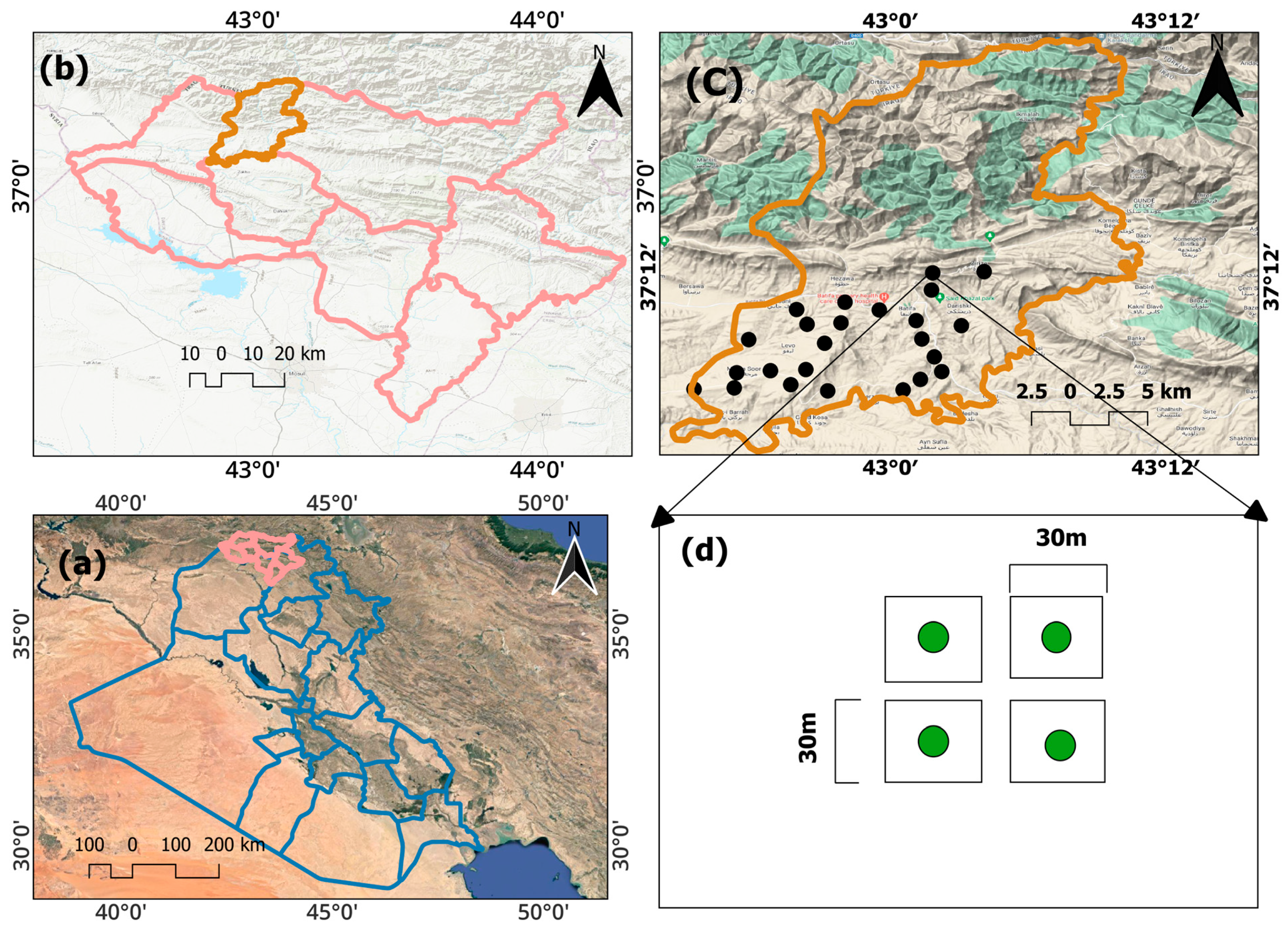
2.1. Study Area
2.2. Dataset and Pre-Processing

| Explanatory Variable | Formula | Reference |
|---|---|---|
| Digital Elevation Models (DEM) | Shuttle Radar Topography Mission (SRTM) from (https://earthexplorer.usgs.gov/, accessed on 20 August 2021) | |
| Landsat 8 (OLI) | b 1: Coastal aerosol, b 2: Blue, b 3: Green, b 4: Red, b 5: NIR, b 6: SWIR 1, b 7: SWIR 2, b 10: TIRS 1, b 11: TIRS 2 | (https://earthexplorer.usgs.gov/, accessed on 22 October 2021) |
| Normalized Difference Vegetation Index | [31] | |
| Soil-Adjusted Vegetation Index | [27] | |
| Brightness Index | [15] |
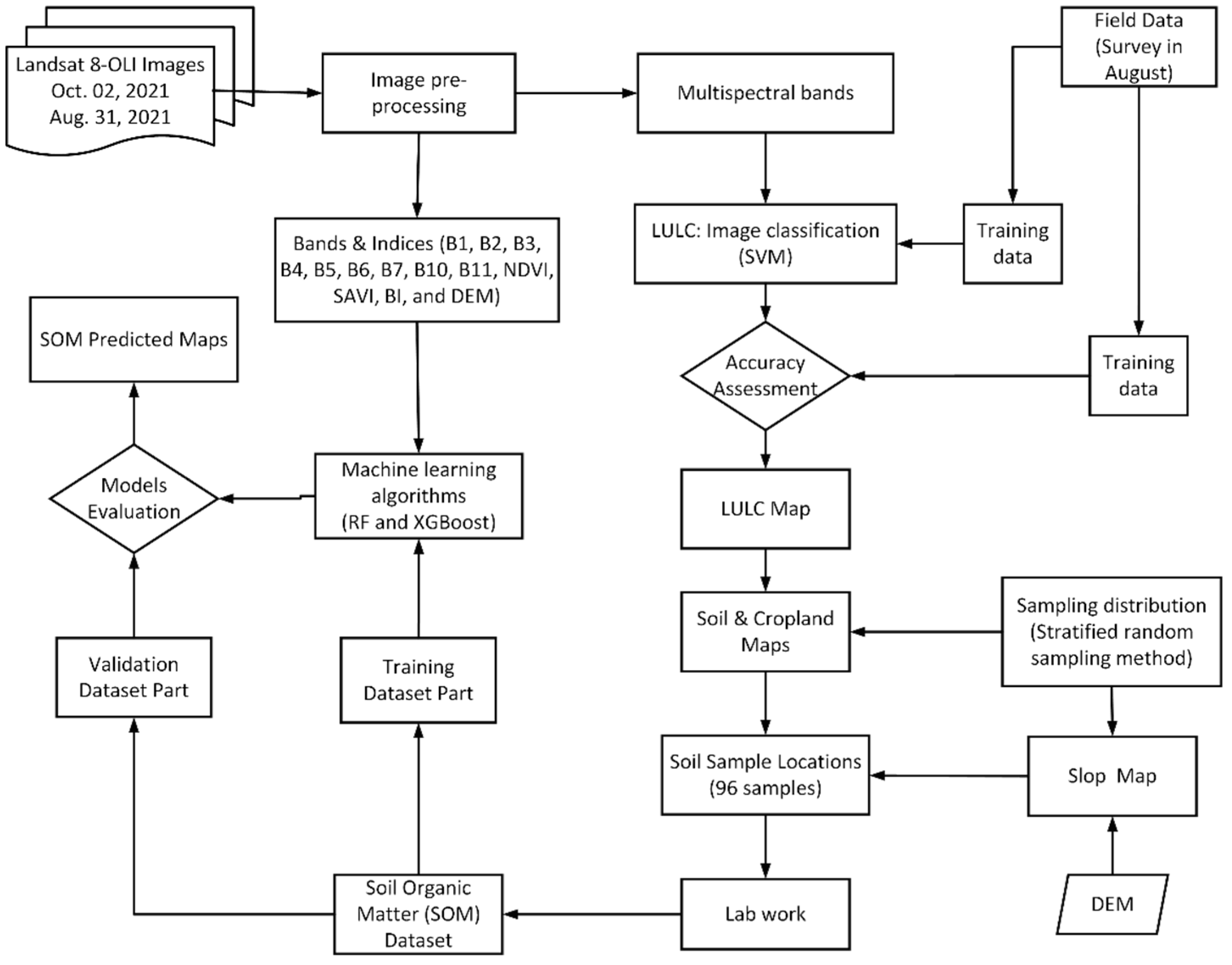
3. Methodology
3.1. LULC and Accuracy Assessment
3.2. RF
3.3. XGBoost
3.4. Validation of ML Models
4. Results and Discussions
4.1. Descriptive Statistics
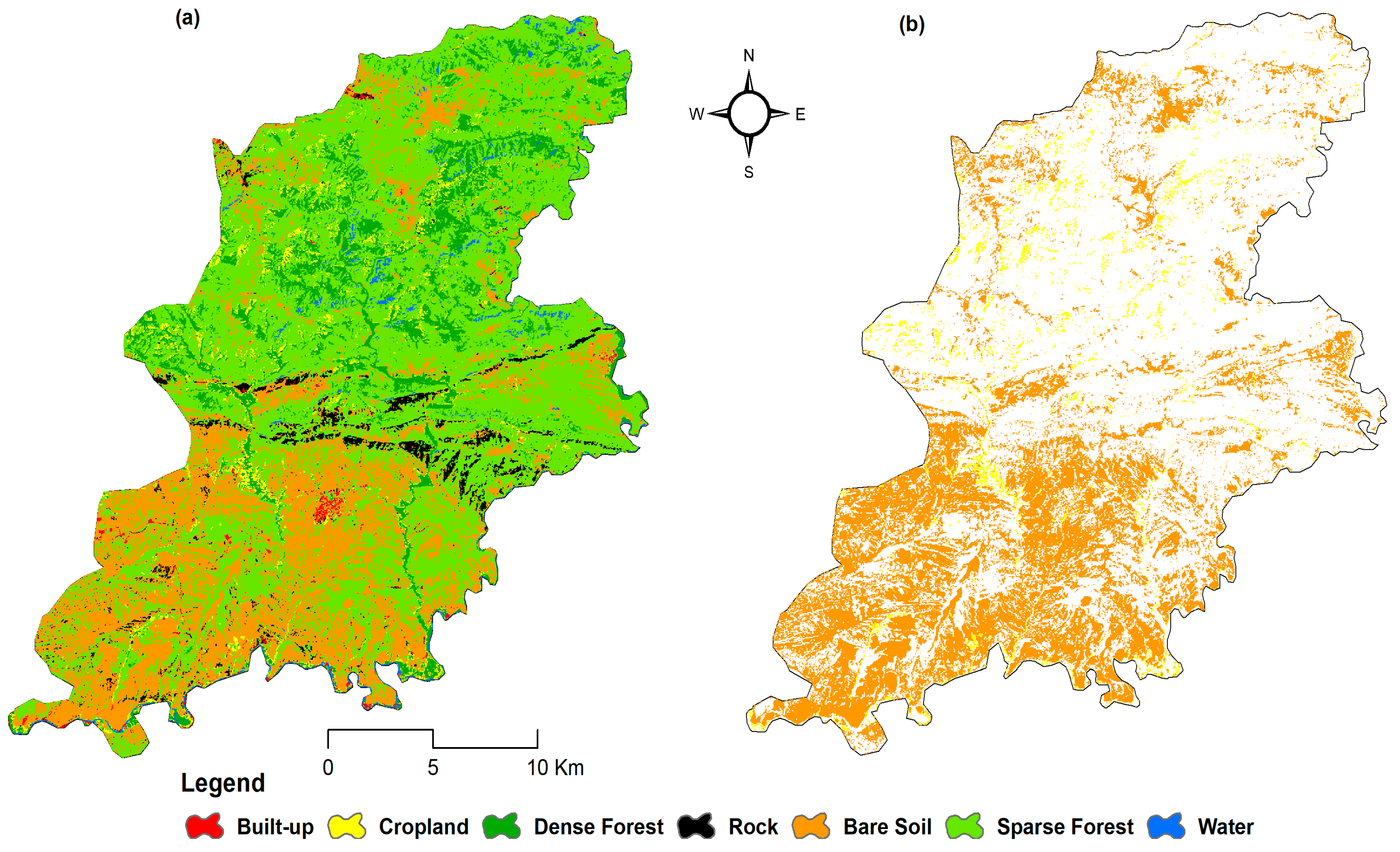
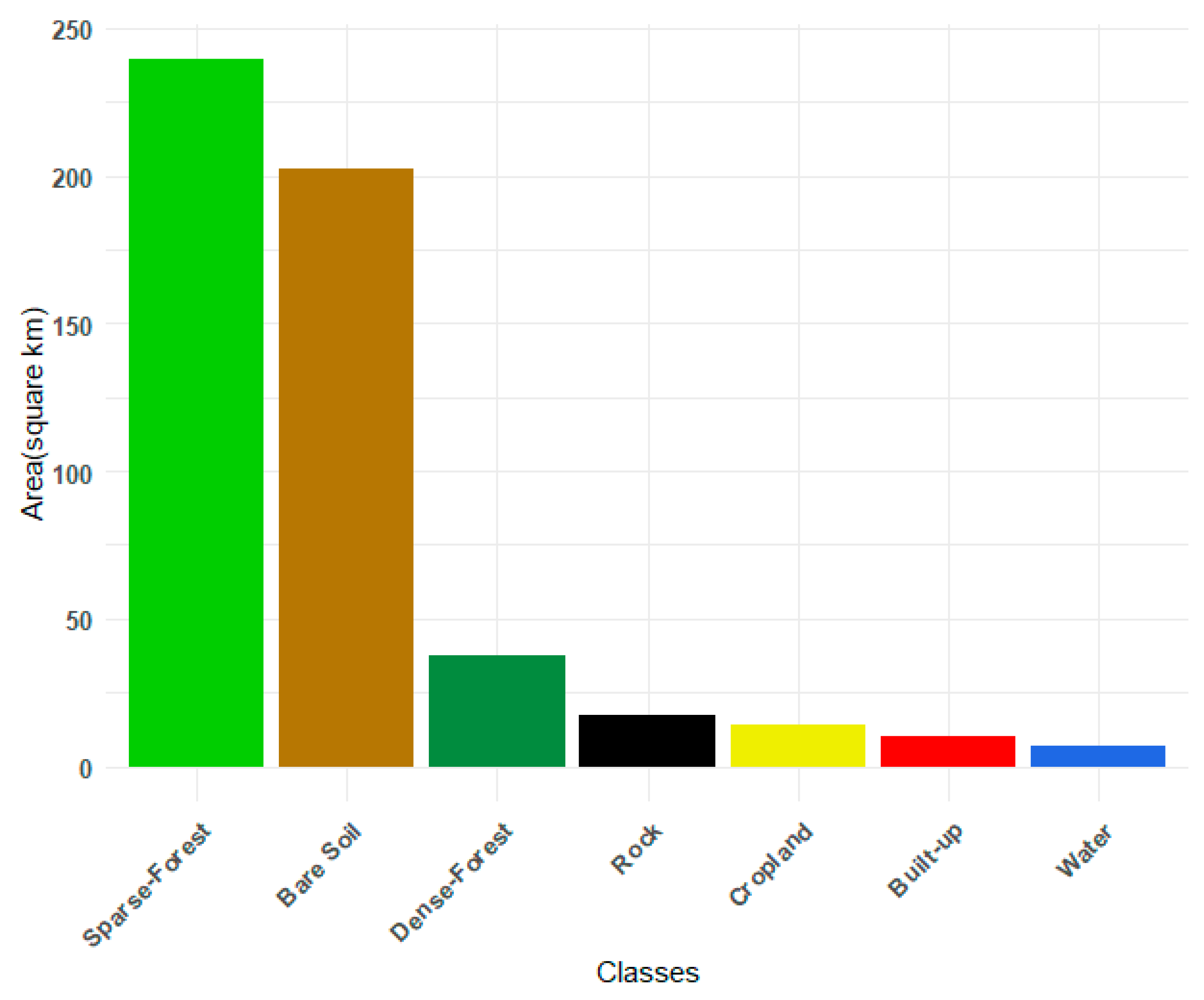
4.2. LULC and Assembled Bare Soil and Cropland Maps
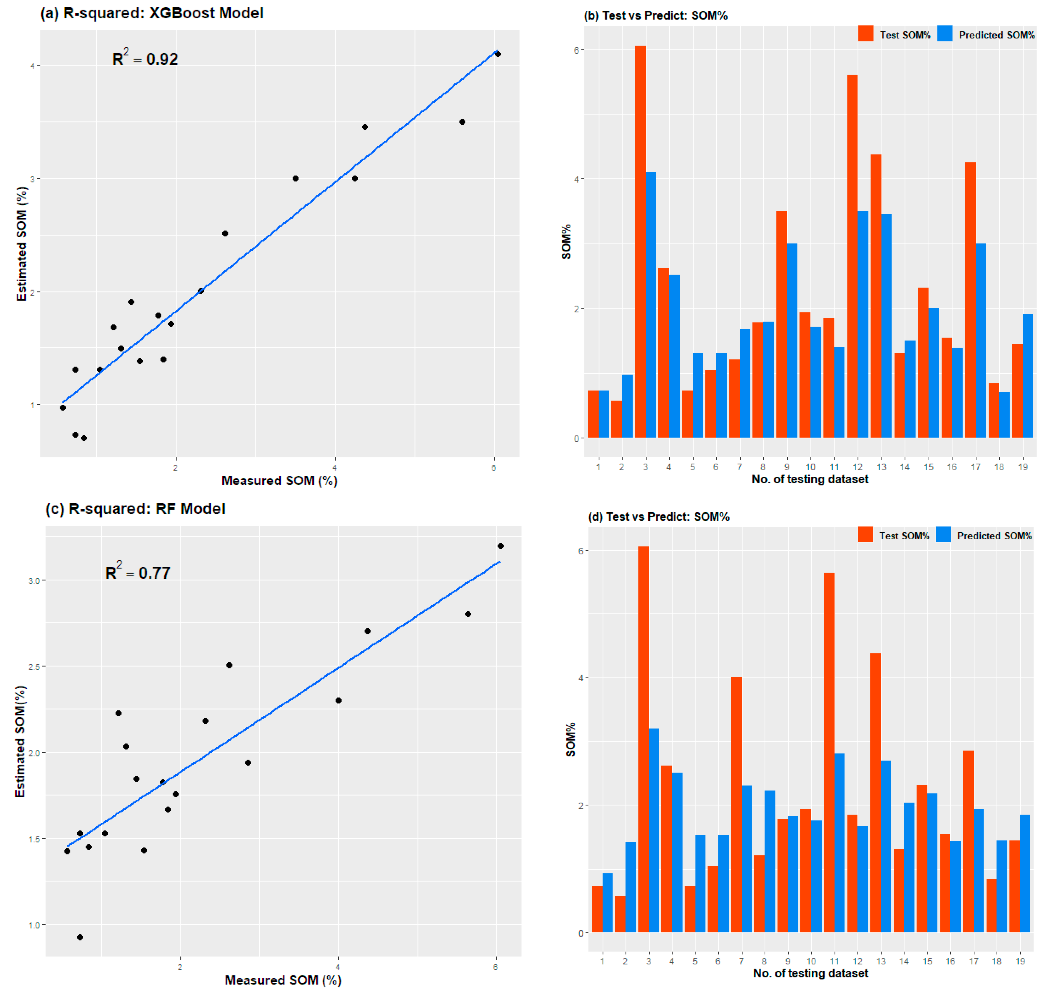
4.3. Model Performance
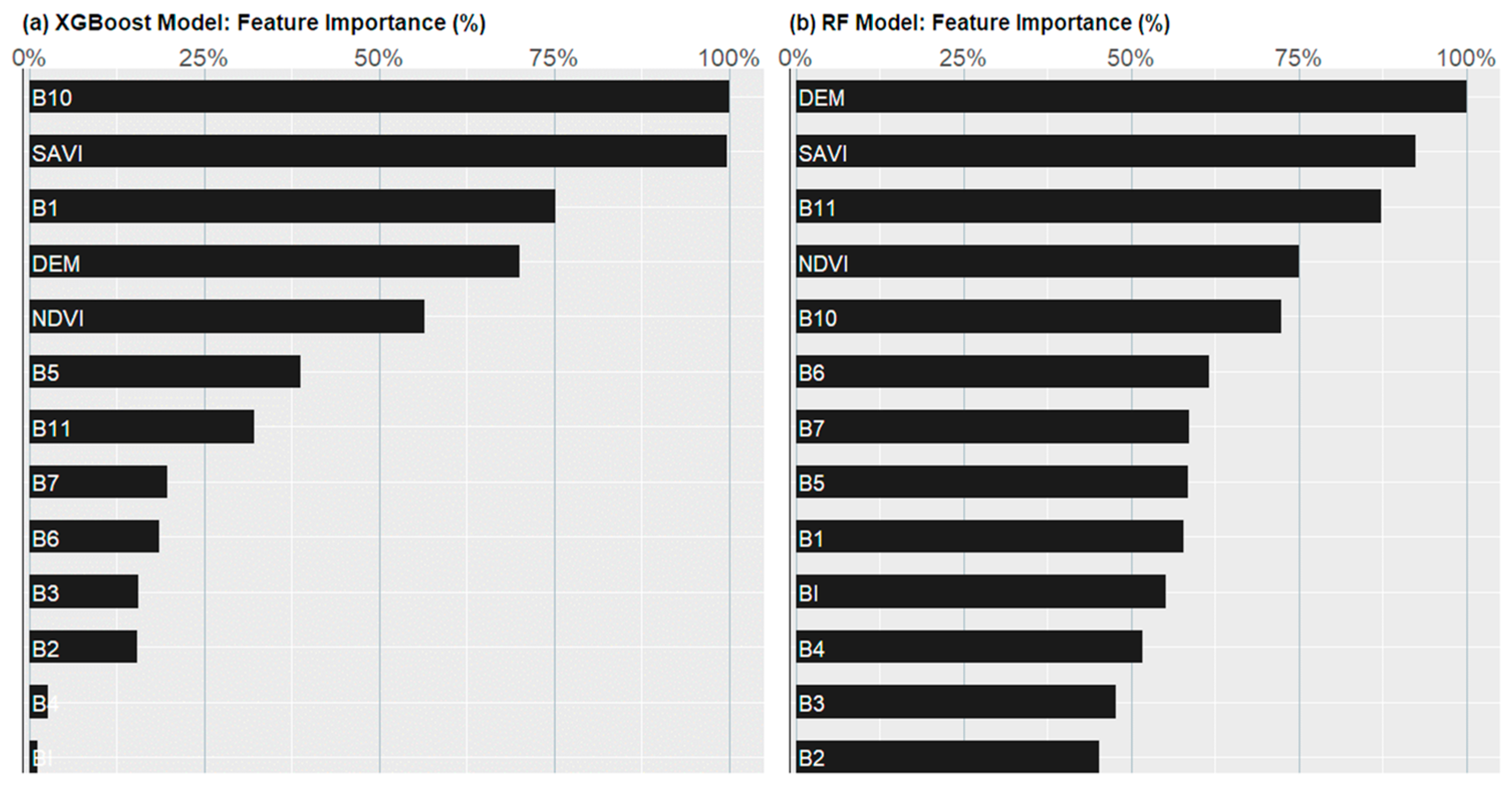
4.4. Variable Importance Analysis
5. Conclusions
- XGBoost exhibited the best performance (R2 = 0.92) compared to RF (R2 = 0.77).
- The RMSE value of the XGBoost model for SOM (RMSE = 0.62) was lower than that of the RF model (RMSE = 0.96), indicating that XGBoost could estimate SOM levels more accurately.
- In XGBoost, Band 10 was found to be the most important variable for predicting SOM, whereas in RF, DEM was the most significant variable.
- The application of our ML model to the entire study area revealed that the SOM’s spatial distribution indicated higher predicted values predominantly in the central and southern regions, despite the field survey not encompassing the northern region.
Author Contributions
Funding
Institutional Review Board Statement
Informed Consent Statement
Data Availability Statement
Conflicts of Interest
References
- McKenzie, N.; Cresswell, H.; Ryan, P.; Grundy, M. Contemporary land resource survey requires improvements in direct soil measurement. Commun. Soil Sci. Plant Anal. 2000, 31, 1553–1569. [Google Scholar] [CrossRef]
- Thomasson, J.; Sui, R.; Cox, M.; Al–Rajehy, A. Soil reflectance sensing for determining soil properties in precision agriculture. Trans. ASAE 2001, 44, 1445. [Google Scholar]
- Ivanov, M.; Abdullin, H.; Gainullin, I.; Gafurov, A.; Usmanov, B.; Williamson, J. Using XVIII–XIX Cent. Maps and Modern Remote Sensing Data for Detecting the Changes in the Land Use at Bulgarian Fortified Settlements in the Volga Region. Earth 2021, 2, 51–65. [Google Scholar] [CrossRef]
- Wilcox, C.H.; Frazier, B.E.; Ball, S.T. Relationship between soil organic carbon and Landsat TM data in Eastern Washington. Photogramm. Eng. Remote Sens. 1994, 60, 777–781. [Google Scholar]
- Chen, F.; Kissel, D.E.; West, L.T.; Adkins, W. Field—Scale mapping of surface soil organic carbon using remotely sensed imagery. Soil Sci. Soc. Am. J. 2000, 64, 746–753. [Google Scholar] [CrossRef]
- Fox, G.A.; Sabbagh, G.J. Estimation of soil organic matter from red and near-infrared remotely sensed data using a soil line Euclidean distance technique. Soil Sci. Soc. Am. J. 2002, 66, 1922–1929. [Google Scholar] [CrossRef]
- Tziachris, P.; Aschonitis, V.; Chatzistathis, T.; Papadopoulou, M. Assessment of spatial hybrid methods for predicting soil organic matter using DEM derivatives and soil parameters. Catena 2019, 174, 206–216. [Google Scholar] [CrossRef]
- Mallick, J.; Ahmed, M.; Alqadhi, S.D.; Falqi, I.I.; Parayangat, M.; Singh, C.K.; Rahman, A.; Ijyas, T. Spatial stochastic model for predicting soil organic matter using remote sensing data. Geocarto Int. 2022, 37, 413–444. [Google Scholar]
- Guo, L.; Sun, X.; Fu, P.; Shi, T.; Dang, L.; Chen, Y.; Linderman, M.; Zhang, G.; Zhang, Y.; Jiang, Q. Mapping soil organic carbon stock by hyperspectral and time-series multispectral remote sensing images in low-relief agricultural areas. Geoderma 2021, 398, 115118. [Google Scholar]
- Wang, S.; Gao, J.; Zhuang, Q.; Lu, Y.; Gu, H.; Jin, X. Multispectral remote sensing data are effective and robust in mapping regional forest soil organic carbon stocks in a northeast forest region in China. Remote Sens. 2020, 12, 393. [Google Scholar] [CrossRef]
- Nawar, S.; Mouazen, A. On-line vis-NIR spectroscopy prediction of soil organic carbon using machine learning. Soil Tillage Res. 2019, 190, 120–127. [Google Scholar] [CrossRef]
- Bian, Z.; Guo, X.; Wang, S.; Zhuang, Q.; Jin, X.; Wang, Q.; Jia, S. Applying statistical methods to map soil organic carbon of agricultural lands in northeastern coastal areas of China. Arch. Agron. Soil Sci. 2019, 66, 532–544. [Google Scholar]
- Song, J.; Gao, J.; Zhang, Y.; Li, F.; Man, W.; Liu, M.; Wang, J.; Li, M.; Zheng, H.; Yang, X.; et al. Estimation of Soil Organic Carbon Content in Coastal Wetlands with Measured VIS-NIR Spectroscopy Using Optimized Support Vector Machines and Random Forests. Remote Sens. 2022, 14, 4372. [Google Scholar] [CrossRef]
- Pal, S.; Sharma, P. A Review of Machine Learning Applications in Land Surface Modeling. Earth 2021, 2, 174–190. [Google Scholar] [CrossRef]
- Xie, B.; Ding, J.; Ge, X.; Li, X.; Han, L.; Wang, Z. Estimation of soil organic carbon content in the Ebinur Lake wetland, Xinjiang, China, based on multisource remote sensing data and ensemble learning algorithms. Sensors 2022, 22, 2685. [Google Scholar] [CrossRef]
- Liang, Z.; Chen, S.; Yang, Y.; Zhou, Y.; Shi, Z. High-resolution three-dimensional mapping of soil organic carbon in China: Effects of SoilGrids products on national modeling. Sci. Total Environ. 2019, 685, 480–489. [Google Scholar] [CrossRef]
- Breiman, L. Random forests. Mach. Learn. 2001, 45, 5–32. [Google Scholar] [CrossRef]
- Gravi, K.A.; Ibrahim, S.M. A Studying the Possibility of Estimating Soil Organic Carbon of Soils under Pinus brutia and Quercus aegilops L. Trees in Sarke-Duhok By Using ASD FieldSpec 3 Spectroradiometer. Sci. J. Univ. Zakho 2020, 8, 34–41. [Google Scholar] [CrossRef]
- Maulood, P.M. Determination of Organic Matter by Using Titrimetric and Loss on Ignition Methods for Northern Iraqi Governorates Soils. Al-Nahrain J. Sci. 2022, 25, 1–7. [Google Scholar] [CrossRef]
- Meshabaz, R.A.; Umer, M.I. Assessment of industrial effluent impacts on soil physiochemical properties in Kwashe Industrial Area, Iraq Kurdistan Region. In Proceedings of the IOP Conference Series: Earth and Environmental Science, Sulaimani, Iraq, 1–4 October 2022; p. 012037. [Google Scholar]
- Yousif, B.S.; Mustafa, Y.T.; Fayyadh, M.A. Digital mapping of soil-texture classes in Batifa, Kurdistan Region of Iraq, using machine-learning models. Earth Sci. Inform. 2023, 16, 1687–1700. [Google Scholar] [CrossRef]
- Mustafa, Y.T.; Ismail, D.R. Land use land cover change in Zakho District, Kurdistan Region, Iraq: Past, current and future. In Proceedings of the 2019 International Conference on Advanced Science and Engineering (ICOASE), Duhok, Iraq, 2–4 April 2019; pp. 141–146. [Google Scholar]
- Buday, T.; Jasim, S.Z. The Regional Geology of Iraq, Tectonism, Magmatism and Metamorphism; Directorate General for Geological Survey: Baghadad, Iraq, 1980; p. 352. [Google Scholar]
- Fayyadh, M.A.; Sindi, A.A.M. Distribution of total carbonate and iron oxides on catena at Duhok Governorate, Kurdistan Region, Iraq. Mater. Today Proc. 2021, 42, 2064–2070. [Google Scholar] [CrossRef]
- Buringh, P. Soils and Soil Conditions in Iraq; Ministry of Agriculture Baghdad: Baghdad, Iraq, 1960. [Google Scholar]
- Wang, S.; Zhuang, Q.; Wang, Q.; Jin, X.; Han, C. Mapping stocks of soil organic carbon and soil total nitrogen in Liaoning Province of China. Geoderma 2017, 305, 250–263. [Google Scholar]
- Sripada, R.P.; Heiniger, R.W.; White, J.G.; Meijer, A.D. Aerial color infrared photography for determining early in—Season nitrogen requirements in corn. Agron. J. 2006, 98, 968–977. [Google Scholar] [CrossRef]
- Walkley, A.; Black, I.A. An examination of the Degtjareff method for determining soil organic matter, and a proposed modification of the chromic acid titration method. Soil Sci. 1934, 37, 29–38. [Google Scholar] [CrossRef]
- Barwari, V.; Hashim, F.A.; Mohammed, B.H. Comparison between Walkley-Black and Loss-on-Ignition methods for organic carbon estimation in soil from different locations. Kufa J. Agric. Sci. 2017, 9, 292–306. [Google Scholar]
- Shamrikova, E.; Kondratenok, B.; Tumanova, E.; Vanchikova, E.; Lapteva, E.; Zonova, T.; Lu-Lyan-Min, E.; Davydova, A.; Libohova, Z.; Suvannang, N. Transferability between soil organic matter measurement methods for database harmonization. Geoderma 2022, 412, 115547. [Google Scholar]
- Rouse, J.W., Jr.; Haas, R.H.; Deering, D.; Schell, J.; Harlan, J.C. Monitoring the Vernal Advancement and Retrogradation (Green Wave Effect) of Natural Vegetation; Texas A&M University Remote Sensing Center: College Station, TX, USA, 1974. [Google Scholar]
- Mather, P.; Tso, B. Classification Methods for Remotely Sensed Data; CRC Press: Boca Raton, FL, USA, 2016. [Google Scholar]
- Thakur, R.; Panse, P. Classification Performance of Land Use from Multispectral Remote Sensing Images using Decision Tree, K-Nearest Neighbor, Random Forest and Support Vector Machine Using EuroSAT Data. Int. J. Intell. Syst. Appl. Eng. 2022, 10, 67–77. [Google Scholar]
- de Santana, F.B.; de Souza, A.M.; Poppi, R.J. Visible and near infrared spectroscopy coupled to random forest to quantify some soil quality parameters. Spectrochim. Acta Part A Mol. Biomol. Spectrosc. 2018, 191, 454–462. [Google Scholar] [CrossRef]
- Wiesmeier, M.; Barthold, F.; Blank, B.; Kögel-Knabner, I. Digital mapping of soil organic matter stocks using Random Forest modeling in a semi-arid steppe ecosystem. Plant Soil 2011, 340, 7–24. [Google Scholar]
- Iqbal, F.; Lucieer, A.; Barry, K. Poppy crop capsule volume estimation using UAS remote sensing and random forest regression. Int. J. Appl. Earth Obs. Geoinf. 2018, 73, 362–373. [Google Scholar] [CrossRef]
- Siroky, D.S. Navigating random forests and related advances in algorithmic modeling. Stat. Surv. 2009, 3, 147–163. [Google Scholar] [CrossRef]
- Chen, T.; Guestrin, C. Xgboost: A scalable tree boosting system. In Proceedings of the 22nd ACM SIGKDD International Conference on Knowledge Discovery and Data Mining, San Francisco, CA, USA, 13 August 2016; pp. 785–794. [Google Scholar]
- Fan, J.; Wang, X.; Wu, L.; Zhou, H.; Zhang, F.; Yu, X.; Lu, X.; Xiang, Y. Comparison of Support Vector Machine and Extreme Gradient Boosting for predicting daily global solar radiation using temperature and precipitation in humid subtropical climates: A case study in China. Energy Convers. Manag. 2018, 164, 102–111. [Google Scholar] [CrossRef]
- Liaw, A.; Wiener, M. Classification and regression by randomForest. R News 2002, 2, 18–22. [Google Scholar]
- Kuhn, M. Building Predictive Models in R Using the caret Package. J. Stat. Softw. 2008, 28, 1–26. [Google Scholar] [CrossRef]
- Hijmans, R.J.; Van Etten, J.; Cheng, J.; Mattiuzzi, M.; Sumner, M.; Greenberg, J.A.; Lamigueiro, O.P.; Bevan, A.; Racine, E.B.; Shortridge, A. Package ‘raster’. R Package 2015, 734, 473. [Google Scholar]
- Wilding, L. Spatial variability: Its documentation, accomodation and implication to soil surveys. In Proceedings of the Soil Spatial Variability, Las Vegas, NV, USA, 30 November–1 December 1985; pp. 166–194. [Google Scholar]
- Wang, K.; Qi, Y.; Guo, W.; Zhang, J.; Chang, Q. Retrieval and mapping of soil organic carbon using Sentinel-2A spectral images from bare cropland in autumn. Remote Sens. 2021, 13, 1072. [Google Scholar] [CrossRef]
- Foody, G.M. Thematic map comparison. Photogramm. Eng. Remote Sens. 2004, 70, 627–633. [Google Scholar] [CrossRef]
- Keskin, H.; Grunwald, S.; Harris, W.G. Digital mapping of soil carbon fractions with machine learning. Geoderma 2019, 339, 40–58. [Google Scholar] [CrossRef]
- Hengl, T.; Leenaars, J.G.; Shepherd, K.D.; Walsh, M.G.; Heuvelink, G.B.; Mamo, T.; Tilahun, H.; Berkhout, E.; Cooper, M.; Fegraus, E. Soil nutrient maps of Sub-Saharan Africa: Assessment of soil nutrient content at 250 m spatial resolution using machine learning. Nutr. Cycl. Agroecosyst. 2017, 109, 77–102. [Google Scholar] [CrossRef]
- Ramcharan, A.; Hengl, T.; Nauman, T.; Brungard, C.; Waltman, S.; Wills, S.; Thompson, J. Soil property and class maps of the conterminous United States at 100-meter spatial resolution. Soil Sci. Soc. Am. J. 2018, 82, 186–201. [Google Scholar] [CrossRef]
- Chen, S.; Liang, Z.; Webster, R.; Zhang, G.; Zhou, Y.; Teng, H.; Hu, B.; Arrouays, D.; Shi, Z. A high-resolution map of soil pH in China made by hybrid modelling of sparse soil data and environmental covariates and its implications for pollution. Sci. Total Environ. 2019, 655, 273–283. [Google Scholar] [CrossRef]
- Hengl, T.; Mendes de Jesus, J.; Heuvelink, G.B.; Ruiperez Gonzalez, M.; Kilibarda, M.; Blagotić, A.; Shangguan, W.; Wright, M.N.; Geng, X.; Bauer-Marschallinger, B. SoilGrids250m: Global gridded soil information based on machine learning. PLoS ONE 2017, 12, e0169748. [Google Scholar] [CrossRef] [PubMed]
- Shangguan, W.; Hengl, T.; Mendes de Jesus, J.; Yuan, H.; Dai, Y. Mapping the global depth to bedrock for land surface modeling. J. Adv. Model. Earth Syst. 2017, 9, 65–88. [Google Scholar] [CrossRef]
- Pahlavan-Rad, M.R.; Dahmardeh, K.; Brungard, C. Predicting soil organic carbon concentrations in a low relief landscape, eastern Iran. Geoderma Reg. 2018, 15, e00195. [Google Scholar] [CrossRef]
- Mirzaee, S.; Ghorbani-Dashtaki, S.; Mohammadi, J.; Asadi, H.; Asadzadeh, F. Spatial variability of soil organic matter using remote sensing data. Catena 2016, 145, 118–127. [Google Scholar] [CrossRef]
- Ning, L.; Cheng, C.; Lu, X.; Shen, S.; Zhang, L.; Mu, S.; Song, Y. Improving the Prediction of Soil Organic Matter in Arable Land Using Human Activity Factors. Water 2022, 14, 1668. [Google Scholar] [CrossRef]
- Zhou, Y.; Hartemink, A.E.; Shi, Z.; Liang, Z.; Lu, Y. Land use and climate change effects on soil organic carbon in North and Northeast China. Sci. Total Environ. 2019, 647, 1230–1238. [Google Scholar] [CrossRef]
- Zhang, Y.; Kou, C.; Liu, M.; Man, W.; Li, F.; Lu, C.; Song, J.; Song, T.; Zhang, Q.; Li, X.; et al. Estimation of Coastal Wetland Soil Organic Carbon Content in Western Bohai Bay Using Remote Sensing, Climate, and Topographic Data. Remote Sens. 2023, 15, 4241. [Google Scholar] [CrossRef]
- Nabiollahi, K.; Eskandari, S.; Taghizadeh-Mehrjardi, R.; Kerry, R.; Triantafilis, J. Assessing soil organic carbon stocks under land-use change scenarios using random forest models. Carbon Manag. 2019, 10, 63–77. [Google Scholar] [CrossRef]
- Taghizadeh-Mehrjardi, R.; Nabiollahi, K.; Kerry, R. Digital mapping of soil organic carbon at multiple depths using different data mining techniques in Baneh region, Iran. Geoderma 2016, 266, 98–110. [Google Scholar] [CrossRef]
- Wang, H.; Zhang, X.; Wu, W.; Liu, H. Prediction of Soil Organic Carbon under Different Land Use Types Using Sentinel-1/-2 Data in a Small Watershed. Remote Sens. 2021, 13, 1229. [Google Scholar] [CrossRef]

| Variables | Min | Max | Median | Mean | Standard Deviation | CV% |
|---|---|---|---|---|---|---|
| SOM% | 0.10 | 6.18 | 1.69 | 1.81 | 1.22 | 67.45 |
| DEM | 633.00 | 1028.00 | 772.00 | 752.91 | 85.46 | 11.35 |
| NDVI | 0.12 | 0.46 | 0.17 | 0.19 | 0.06 | 31.58 |
| SAVI | 0.09 | 0.30 | 0.12 | 0.13 | 0.03 | 27.34 |
| BI | 0.06 | 0.19 | 0.12 | 0.12 | 0.031 | 24.41 |
| B1 | 0.05 | 0.12 | 0.09 | 0.08 | 0.02 | 19.55 |
| B2 | 0.05 | 0.14 | 0.09 | 0.09 | 0.02 | 23.71 |
| B3 | 0.08 | 0.22 | 0.14 | 0.14 | 0.03 | 25.17 |
| B4 | 0.10 | 0.31 | 0.20 | 0.20 | 0.05 | 25.12 |
| B5 | 0.18 | 0.41 | 0.29 | 0.30 | 0.05 | 19.60 |
| B6 | 0.19 | 0.41 | 0.34 | 0.31 | 0.05 | 17.87 |
| B7 | 0.13 | 0.33 | 0.24 | 0.24 | 0.04 | 18.44 |
| B10 | 34.21 | 43.01 | 39.64 | 39.52 | 1.99 | 5.04 |
| B11 | 33.19 | 41.84 | 38.71 | 38.63 | 1.91 | 4.94 |
| LULC | Classified | |||||||
|---|---|---|---|---|---|---|---|---|
| Dense Forest | Sparse Forest | Rock | Soil | Water | Cropland | Built-Up | User’s Accuracy | |
| Dense Forest | 65 | 1 | 0 | 0 | 0 | 0 | 0 | 98.48 |
| Sparse Forest | 1 | 31 | 0 | 4 | 0 | 0 | 0 | 86.11 |
| Rock | 0 | 0 | 32 | 1 | 0 | 0 | 0 | 96.96 |
| Soil | 0 | 1 | 4 | 60 | 0 | 2 | 0 | 89.55 |
| Water | 1 | 0 | 0 | 0 | 14 | 0 | 0 | 93.33 |
| Cropland | 0 | 0 | 0 | 1 | 0 | 19 | 0 | 95 |
| Built-up | 0 | 0 | 1 | 0 | 1 | 0 | 18 | 90 |
| Producer’s Accuracy | 97.01 | 93.93 | 86.48 | 90.90 | 93.33 | 95 | 100 | |
| Overall Accuracy | 93% | |||||||
| Kappa Coefficient | 0.91 | |||||||
| ML Algorithms | MAE | RMSE | R2 |
|---|---|---|---|
| XGBoost | 0.41 | 0.62 | 0.92 |
| RF | 0.65 | 0.96 | 0.77 |
Disclaimer/Publisher’s Note: The statements, opinions and data contained in all publications are solely those of the individual author(s) and contributor(s) and not of MDPI and/or the editor(s). MDPI and/or the editor(s) disclaim responsibility for any injury to people or property resulting from any ideas, methods, instructions or products referred to in the content. |
© 2023 by the authors. Licensee MDPI, Basel, Switzerland. This article is an open access article distributed under the terms and conditions of the Creative Commons Attribution (CC BY) license (https://creativecommons.org/licenses/by/4.0/).
Share and Cite
Khalaf, H.S.; Mustafa, Y.T.; Fayyadh, M.A. Digital Mapping of Soil Organic Matter in Northern Iraq: Machine Learning Approach. Appl. Sci. 2023, 13, 10666. https://doi.org/10.3390/app131910666
Khalaf HS, Mustafa YT, Fayyadh MA. Digital Mapping of Soil Organic Matter in Northern Iraq: Machine Learning Approach. Applied Sciences. 2023; 13(19):10666. https://doi.org/10.3390/app131910666
Chicago/Turabian StyleKhalaf, Halmat S., Yaseen T. Mustafa, and Mohammed A. Fayyadh. 2023. "Digital Mapping of Soil Organic Matter in Northern Iraq: Machine Learning Approach" Applied Sciences 13, no. 19: 10666. https://doi.org/10.3390/app131910666
APA StyleKhalaf, H. S., Mustafa, Y. T., & Fayyadh, M. A. (2023). Digital Mapping of Soil Organic Matter in Northern Iraq: Machine Learning Approach. Applied Sciences, 13(19), 10666. https://doi.org/10.3390/app131910666