Regime-Specific Quant Generative Adversarial Network: A Conditional Generative Adversarial Network for Regime-Specific Deepfakes of Financial Time Series

Abstract

Simulating financial time series (FTS) data consistent with non-stationary, empirical market behaviour is difficult, but it has valuable applications for financial risk management. A better risk estimation can improve returns on capital and capital efficiency in investment decision making. Challenges to modelling financial risk in market crisis environments are anomalous asset price behaviour and a lack of historical data to learn from. This paper proposes a novel semi-supervised approach for generating regime-specific ‘deep fakes’ of FTS data using generative adversarial networks (GANs). The proposed architecture, a regime-specific Quant GAN (RSQGAN), is a conditional GAN (cGAN) that generates class-conditional synthetic asset return data. Conditional class labels correspond to distinct market regimes that have been detected using a structural breakpoint algorithm to segment FTS into regime classes for simulation. Our RSQGAN approach accurately simulated univariate time series behaviour consistent with specific empirical regimes, outperforming equivalently configured unconditional GANs trained only on crisis regime data. To evaluate the RSQGAN performance for simulating asset return behaviour during crisis environments, we also propose four test metrics that are sensitive to path-dependent behaviour and are also actionable during a crisis environment. Our RSQGAN model design borrows from innovation in the image GAN domain by enabling a user-controlled hyperparameter for adjusting the fit of synthetic data fidelity to real-world data; however, this is at the cost of synthetic data variety. These model features suggest that RSQGAN could be a useful new tool for understanding risk and making investment decisions during a time of market crisis.

1. Introduction

Employing machine learning tasks to successfully model financial time series (FTS) data (e.g., stock prices, FX rates) is a challenging but valuable exercise [1]. For example, a supervised learning model for predicting future asset returns may be used to make directional investment decisions (i.e., a bet on the future direction of an asset’s price, or to prioritise and weight trades). However, there are difficulties in the FTS data domain that make supervised learning tasks more challenging than other domains: (1) a lack of training data versus other data domains, e.g., images, video, text, audio, etc., which results in higher model estimation and generalisation errors, thus degrading performance, and (2) persistently low signal-to-noise ratios, as market efficiency dampens detectable signals [2].

Another valuable machine learning task for aiding investment decision making is to learn the data distribution of the underlying data generation process (DGP) [3]. Generative models could be used to simulate the evolution of FTS data and help investment and risk professionals make better risk-based investment decisions (i.e., approaches to hedging or assessing risk–reward trade-offs) and improve capital efficiency.

Generative modelling approaches, such as variational auto-encoders (VAEs) [4,5] and generative adversarial networks (GANs) [6], have been used for DGP simulation tasks in other domains. In the image domain, GANs are known to be more successful than VAEs in generating ‘sharper’ synthetic data when compared to VAE-based approaches [7,8].

In the FTS domain, GANs have only recently been explored for simulating FTS data [9,10,11,12,13,14,15,16,17].

A key issue when training predictive or generative FTS models in real-world settings is the non-stationary behaviour of the FTS data domain. Non-stationarity in asset return behaviours is a feature of complex market systems, driven by exogenous factors (e.g., government policies, interventions, regulations, industry structural changes) and endogenous factors (e.g., market expectations, participant behaviour, feedback loops, and dynamic algorithms). Market participants often describe a contiguous period of persistent market behaviours (e.g., directions, volatilities, correlations) as a market ‘regime’. A regime change is a significant DGP feature that contributes to the non-stationarity of observed FTS data.

The performance of predictive or generative FTS models significantly depends on whether future data will be drawn from the same DGP as the training period. However, regime class imbalance has often been overlooked in FTS model training. Failure to account for this feature could lead to ‘unconditional’ models being trained in ‘mixed-regime’ environments and not be reflective of the modeller’s explicit expectations for current or future regimes.

This paper proposes a novel approach to the generative modelling of regime-specific FTS data by using conditional generative adversarial networks (cGANs) [18]. The application of cGANs to the FTS domain enables the class-conditional simulation of asset price behaviour that may be characteristic of historic market regime environments, such as past financial crises. The key benefits are that (1) users would have the flexibility to simulate market behaviours not dependent on recent regime conditions if conditions have changed or are changing and (2) it gives users the flexibility to explicitly simulate mixture models by generating class-conditional synthetic data and weighting their prevalence with regime class priors.

Few papers in the FTS GAN literature have applied a cGAN to modelling FTS data. Each of these studies demonstrated a range of conditioning approaches. Fu et al. [15] used categorical, ordinal, or continuous conditioning representations to learn toy Gaussian mixtures and vector autoregression (VAR) processes. Koshiyama et al. [13] conditioned on a time series of recent returns, and de Meer Pardo [14] conditioned on current VIX levels and also on a time series of a ‘principal’ asset returns for generating multivariate FTS data for multiple assets.

However, none of these approaches directly address the empirical issue of regime imbalance in the training data. Fu et al. [15] partially addressed this by selecting a balanced time period between 2007 and 2011 based on heuristical domain knowledge but did not utilise a larger volume of data available for learning. Koshiyama et al. [13] conditioned on the most recent 252 trading days (1 year) of recent historical returns using training data between 2001 and 2013 to generate 1260 days (5 years) of data to assess the training strategy performance. de Meer Pardo [14] used 100 days of historical S&P500 data as a conditioning variable between 2004 and 2015 to generate joint S&P500 and VIX data.

To address regime imbalance and learning a generative model specific to a particular historical regime, we propose a novel approach called a regime-specific Quant GAN (RSQGAN). RSQGAN is a conditional GAN [18] for FTS that extends the Quant GAN (QGAN) model [12] demonstrated for modelling unconditional FTS data.

In addition, the aforementioned cGAN studies for FTS data used GAN quality evaluation measures tailored for specific commercial applications: (1) the fine-tuning of trading strategies and/or data augmentation for training trading strategies to maximise risk-adjusted returns [13]; (2) value at risk and expected shortfall estimation [15]; and (3) implicit evidence that cGAN-generated synthetic data augments training data sets and improves the out-of-sample discriminator performance [14,19].

To directly assess synthetic data quality, particularly for ‘crisis’ regimes, a number of key evaluation criteria are proposed to assess the improvement in the quality of capturing path-dependent time series behaviour in these regimes so they might be acted on in real-world risk management contexts.

The contributions of this paper to existing FTS GAN approaches are threefold:

• The use of a structural breakpoint algorithm, greedy Gaussian segmentation [20], to learn time-dependent class categories (‘regimes’) to be used as embedding conditions and cluster time series data in pre-processing to train the conditional RSQGAN;
• A user-controlled hyper-parameter method in RSQGAN topological design (‘z-clipping’) as originally proposed by Brock et al. [21] in BigGAN, which enables users to directly control the variability of synthetic data outputs; and
• An empirical evaluation of the selection of GAN performance metrics for specifically evaluating synthetic FTS data quality for rarer crisis regimes.

This paper demonstrates that RSQGAN is able to achieve improvements across multiple quality evaluation metrics for synthetic crisis regime data, relative to an unconditional QGAN [12] model using the same topology but exclusively trained on crisis regime data. This suggests that the RSQGAN model can learn a useful crisis regime embedding representation and benefits from parameter sharing by learning useful time series features from the behaviour of majority (non-crisis) regime classes.

The rest of this paper is structured as follows. In Section 2, we give a high-level overview of GANs and key issues encountered in training. In Section 3, highlights are (i) an overview of the GAN research literature and (ii) innovations in image GAN architecture relevant to developing the RSQGAN architecture. In Section 4, an overview is provided of research papers demonstrating the application of GANs to the FTS data domain.

In Section 5, the structural breakpoint algorithm, greedy Gaussian segmentation (GGS) [20], for segmenting time series into regimes for class encoding is briefly described. A description of the RSQGAN model, which evolved from the QGAN model [12] and its training procedure, is described. The section concludes with an outline of data and experimental methodologies.

In Section 6 and Section 7, interpretations of experimental results are provided, along with other explanatory observations. In Section 8 and Section 9, proposed future work is suggested to address current methodological limitations, and key insights are summarised. Appendix A includes further technical details drawn from key papers.

2. Background

Generative Adversarial Networks (GANs)

Within the family of generative modelling approaches, generative adversarial networks (GANs) [6] are referred to as an example of a likelihood-free inference approach [22] to generative modelling. The learned density of the real DGP X ∼${\mathbb{P}}_{\mathrm{r}}\left(x\right)$ is implicitly known if samples can be generated that are consistent with empirical densities. In contrast, explicit approaches aim to learn parameters of latent variable densities. However, due to their intractability, approximations are needed, which can negatively impact performance [23].

Since the introduction of GANs in 2014 as a novel approach to creating synthetic images, rapid progress has been made in the image domain [21,24,25] and has proliferated across data domains such as audio [26], text [27,28], medical data [19,29], and, more recently, videos [30,31].

The idea behind the original ‘vanilla’ GAN algorithm [6] is the adversarial training of a generator network $G:(z;{\theta }_g)\mapsto \tilde{x}$ against a discriminator network $D:(x;{\theta }_d)\mapsto [0,1]$ that aims to correctly discriminate between generated samples $\tilde{x}$ and real instances x. z is drawn from a random noise prior distribution $p_Z\left(z\right)$, e.g., multinomial standard Gaussian $Z\sim \mathcal{N}(\mu =0,\mathsf{\Sigma }=I)$.

Adversarial training is viewed as a minimax game between G and D, intuitively, when the joint minimax loss function in Equation (1) converges:

$$\underset{G}{min}\underset{D}{max}{\mathbb{E}}_{x\sim {\mathbb{P}}_r\left(x\right)}[logD\left(x\right)]+{\mathbb{E}}_{z\sim p_Z\left(z\right)}[log(1-D\left(G\left(z\right)\right))].$$

(1)

It was shown by Goodfellow et al. [6] that a unique solution at ${\mathbb{P}}_r={\mathbb{P}}_g$ exists when $D^{*}\left(x\right)=\frac{1}{2}$, as optimising Equation (1) under the optimal generator $D^{*}\left(x\right)$ is equivalent to minimising the cost function:

$$-log4+2·JSD({\mathbb{P}}_r\parallel {\mathbb{P}}_g)$$

(2)

where $JSD({\mathbb{P}}_r\parallel {\mathbb{P}}_g)$ is the Jensen–Shannon divergence (JSD) between ${\mathbb{P}}_r$ and ${\mathbb{P}}_g$:

$$JSD({\mathbb{P}}_r\parallel {\mathbb{P}}_g)=KL({\mathbb{P}}_r\parallel \frac{{\mathbb{P}}_r+{\mathbb{P}}_g}{2})+KL({\mathbb{P}}_g\parallel \frac{{\mathbb{P}}_r+{\mathbb{P}}_g}{2})$$

(3)

and $KL({\mathbb{P}}_X\parallel {\mathbb{P}}_Y)$ is the Kullback–Leibler (KL) divergence between ${\mathbb{P}}_X$ and ${\mathbb{P}}_Y$ given by

$$KL\left({\mathbb{P}}_X\parallel {\mathbb{P}}_Y\right)={\int }_{\mathcal{X}}{P}_X\left(x\right)log\frac{P_X\left(x\right)}{P_Y\left(x\right)}dx$$

(4)

over the joint support for $P_{X,Y}$ denoted by $\mathcal{X}$.

However, the training of vanilla GANs has been problematic in practice. Issues include: (1) a lack of variation in simulated outputs (‘mode collapse’), (2) non-convergence during training, and (3) training losses being a poor metric to evaluate GAN output quality.

• Mode collapse. The true data distribution ${\mathbb{P}}_r\left(x\right)$ is likely to be high-dimensional and multi-modal. Mode collapse can occur if, during training, the discriminator network overfits in its ability to identify generated fakes. The generator network then responds by restricting fake samples to modes that are less likely to be classified as fakes. The progressive overfitting of the discriminator within this subset causes the density of generated samples to concentrate into a shrinking support space. Despite this, observed generator and discriminator losses continue to shrink but generated samples become invariant. Conversely, another cause of mode collapse could be from vanishing discriminator gradients, which result in stalled learning for the generator network. Methods for dealing with discriminator overfitting include weight regularisation [32], regularisation by discriminator learning from stochastically corrupted inputs [33], using alternative loss functions such as Wasserstein loss (WGAN) [34] and applying gradient penalties in the discriminator learning process (WGAN-GP) [35].
• Training non-convergence. Though convergence may not indicate training success if mode collapse occurs, non-convergence in the adversarial training of vanilla GANs may also indicate failure. The nature of adversarial training and non-convex joint loss functions can lead to oscillatory behaviour. The oscillatory non-convergence of losses may not produce desirable or stable results for the learned DGP. Therefore, increasingly unstable representations of the DGP could be learned. Non-convergence can also be caused by an underfitting discriminator or vanishing discriminator gradient that results in a generator’s failure to learn. Interested readers are referred to GAN meta-studies that examine the effectiveness of discriminator regularisation and loss functions to manage the non-convergence [36] and critical analysis of theoretical supports for reducing mode collapse and non-convergence in the image data domain [23].
• Quality evaluation. As the above discussion argues that the overall GAN performance cannot be reliably judged by observing training losses, other evaluation metrics would be needed. Evaluation metrics would need to consider variability across modes and output quality for each mode. Subjective human evaluation could apply for data domains such as images or sound, though these are not robust measures for model benchmarking. It was argued by Theis et al. [37] that GANs could be used for a number of purposes (e.g., unsupervised feature learning, density estimation, in-filling, etc.), the quality of a GAN should be evaluated based on its originally intended purpose. However, quantitative evaluation metrics and subjective human assessment measures do not necessarily correlate to the performance of the GAN’s objective. For image GANs, quantitative evaluation methods such as inception score [38] and Fréchet inception distance [39] metrics were developed to correlate with performance for image synthesis tasks. For conditional image GANs, the Fréchet joint distance was proposed by DeVries et al. [40] to explicitly metricate inter-mode variability and intra-mode quality over a joint Gaussian distribution in embedded image and conditioning spaces. By contrast, in the FTS data domain, the GAN output quality cannot easily be subjectively judged by visual inspection. Instead, simulated FTS data are judged with reference to a set of market heuristics called stylised facts [41,42,43] as outlined in Section 5.4 below.

3. Related Work

GANs are a highly active research field. Key research directions include:

• Stability improvements, which deal with issues such as mode collapse and non-convergence;
• Evaluation improvements, which derive numerical measures to evaluate GAN output quality; and
• Architectural improvements, which aim to improve GAN output quality, applied across domains.

Provided below is a brief overview of key GAN research literature.

3.1. Stability Improvements

Theory into the causes of GAN non-convergence and mode collapse was explored by Arjovsky and Bottou [33]. The authors demonstrate that non-convergence occurs by proving that when the distributions ${\mathbb{P}}_r$ and ${\mathbb{P}}_g$ are on low-dimensional manifolds and not perfectly aligned, then there exists a perfect discriminator $D^{*}(x;{\theta }_d)$. They show that as the discriminator D converges toward the perfect discriminator $D^{*}$, generator gradient norms converge to zero, which leads to non-convergence in training. They also demonstrate that mode collapse is caused by large regions of discontinuity or zero values of ${\mathbb{P}}_g$ in the joint support of $\left({\mathbb{P}}_r,{\mathbb{P}}_g\right)$. The authors prove that this assigns a high cost to generating poor fakes and a low cost to mode dropping. Arjovsky et al. [34] thus propose a critic WGAN loss function, derived from the Wasserstein-1 (or earth mover distance) [44], with convergence properties that correlate with an improvement in generator sample quality:

$$\underset{G}{min}\underset{D\in {\mathcal{D}}_1}{max}{\mathbb{E}}_{x\sim {\mathbb{P}}_r}\left[D(x;{\theta }_d)\right]-{\mathbb{E}}_{z\sim p_Z\left(z\right)}\left[D\left(G_{{\theta }_g}\left(z\right)\right)\right]$$

(5)

for a discriminator function D, with sufficient capacity that satisfies the 1-Lipschitz condition denoted by $D\in {\mathcal{D}}_1$.

Arjovsky et al. [34] further observe that, as the critic weights of $D\in {\mathcal{D}}_1$ need to have support in compact metric space, they initially propose weights to be clipped to a chosen hyperparameter region $\mathfrak{W}:\mathfrak{W}\subset {\mathbb{R}}^{dim\left({\theta }_d\right)}$ during training.

Gulrajani et al. [35] observe that the effect of weight clipping in the WGAN formulation [34] results in failure to recognise the WGAN value surface for a fixed generator. Critic gradients are observed to explode or vanish in training. Gulrajani et al. [35] derive the WGAN-GP loss function in Equation (6) below, following proof of gradient properties for some optimal critic $D^{*}$, and conclude that a gradient penalty controlled by hyperparameter ${\lambda }_{GP}$ should be added to the WGAN value function:

$$\underset{G}{min}\underset{D\in {\mathcal{D}}_1}{max}{\mathbb{E}}_{x\sim {\mathbb{P}}_r}\left[D(x;{\theta }_d)\right]-{\mathbb{E}}_{z\sim p_Z\left(z\right)}\left[D\left(G_{{\theta }_g}\left(z\right)\right)\right]+\lambda {\mathbb{E}}_{\widehat{x}\sim {\mathbb{P}}_{\widehat{x}}}\left[{\left(\parallel {\nabla }_{\widehat{x}}D\left(\widehat{x}\right){\parallel }_2-1)\right)}^2\right]$$

(6)

3.2. Evaluation Improvements

The development of automated approaches for evaluating GAN output quality is well established in the image data domain. An overview of GAN evaluation methods in the FTS data domain is covered in Section 4. In principle, evaluation scores should reward both the generation of high intra-mode variability and also high inter-mode separation ‘class label certainty’. The earliest image GAN evaluation metric, inception score [38], measured high intra-mode variability by the high unconditional label entropy of $p\left(\mathcal{C}\right)=\int p\left(\mathcal{C}\right|\tilde{x})d\tilde{x}$ and high inter-mode separation by the low class-conditional label entropy of $p\left(\mathcal{C}\right|\tilde{x})$ determined by feeding generated samples into a pretrained inception model [45]. Heusel et al. [39] argued that, as the inception score approach did not measure scores for synthetic data versus scores for real-world data, a proposed measure of synthetic data quality, the Fréchet inception distance (FID), could examine the Wasserstein-2 [44] distance between high layer feature abstractions of real samples ${\mathbb{P}}_r$ and synthetic samples ${\mathbb{P}}_g$. FID scores were shown to correlate with various forms of induced image noise. This approach was extended to the conditional GAN case by DeVries et al. [40]. The authors observed that though mode class variability is implicitly desired for unconditional GANs, it is explicitly desired for conditional GANs. The proposed Fréchet joint distance (FJD) measures intra-class conditional quality and consistency as well as inter-class conditional diversity. This is measured also using the Wasserstein-2 distance [44] between joint data and class distributions $(x^{\left(i\right)},{\mathcal{C}}^{\left(i\right)}),({\tilde{x}}^{\left(i\right)},{\mathcal{C}}^{\left(i\right)})$.

3.3. Architectural Improvements

Improvements in the GAN research literature that are relevant for designing features of the RSQGAN model include:

• Temporal convolutional networks (TCNs) [12,46]— an improvement in neural architecture for learning time series representations;
• Conditional GANs (cGANs) [18]—an improvement to ensure deliberate generation from distinct class modes;
• ‘z-skipping’ and ‘z-clipping’ [21]—improvements to class conditional synthetic quality, while giving user control to synthetic data size and the ability to explicitly trade off synthetic fidelity to real training data against synthetic variety, respectively.

Temporal convolutional networks (TCNs) [46] are effective in modelling long-range dependencies in sequential data compared to other recurrent network architectures.

Design features of the TCN include dilated causal convolutions, which allow the network to learn time-lag-dependent features at different dilation frequencies, but only caused from prior inputs in the sequence; layered embeddings, which allow representations to be learned at different levels of time scale resolution (i.e., larger receptive fields); and residual connections [47], which improve convergence for deep layered TCN networks. See Figure 1.

Figure 1. Architecture of a TCN. Image and caption credit: Bai et al. [46]. Reproduced with the authors’ permission. (a) A dilated causal convolution with dilation factors $d=1,2,4$ and filter size $k=3$. The receptive field is able to cover all values from the input sequence. (b) A TCN residual block. A 1 × 1 convolution is added with residual input and output having different dimensions. (c) An example of residual connection in a TCN. The blue lines are filters in the residual function and the green lines are identity mappings.

The first known use of TCNs to generate synthetic FTS data was the Quant GAN architecture [12] as described in Section 4 below and in more detail in Appendix A.2 and Appendix A.3.

Conditional GANs [18] aim to explicitly address the issue of mode collapse by directly inducing the generation of class-conditional data. Rather than unconditional generations of $G(z;{\theta }_g)$ from adversarial training against an unconditional discriminator/critic network $D(x;{\theta }_d)$, both generator and discriminator/critic networks can be conditioned against classes ${\mathcal{C}}_j$ to learn $G\left(z\right|{\mathcal{C}}_j;{\theta }_g)$ and $D\left(x\right|{\mathcal{C}}_j;{\theta }_d)$.

The conditional vanilla GAN minimax discriminator loss can thus be expressed as:

$$\underset{G}{min}\underset{D}{max}{\mathbb{E}}_{x\sim {\mathbb{P}}_r\left(x\right)}[logD\left(x\right|{\mathcal{C}}_j)]+{\mathbb{E}}_{z\sim p_Z\left(z\right)}[log(1-D\left(G\left(z\right|{\mathcal{C}}_j)\right))].$$

(7)

The training procedure shown below accepts conditional class ${\mathcal{C}}_j$ as an additional input tensor in training the cGAN network. Another advantage of this approach is that the user can specify the form of the conditions ${\mathcal{C}}_j$ in semi-supervised data generation or apply representations of ${\mathcal{C}}_j$ from an unsupervised learning process.

‘skip-z layers’ and ‘z-clipping’ are two methods applicable to cGANs as described in the single paper by Brock et al. [21]. It explored the effect of larger minibatch sizes in training larger-image cGAN models. Rather than concatenating an encoding of the conditional vector ${\mathcal{C}}_j$ to a noise prior z at the input layer of a network (as seen in Figure 2 above), the noise and class encoding (‘skip-z layers’) are instead introduced at multiple hidden layers. In this way, the network can learn class-conditional feature representations at different receptive field sizes. In addition, this innovation allows for an arbitrarily large noise prior z to be used for the generator input layer, as this no longer requires the topology of the joint noise and class embedding layer to be defined in advance.

Figure 2. Conditional GAN training architecture. Image credit: Mirza and Osindero [18]. Reproduced with the authors’ permission.

Further, Brock et al. [21] test a variety of noise prior distributions other than the standard multinomial uniform and Gaussian distributions. The authors discover that sampling from a truncated normal distribution, i.e., re-sampling the noise prior z if $\left|z\right|\ge z^{clip}$ for some clipping hyperparameter $z^{clip}\ge 0$, would allow users control, indirectly trading off improved fidelity to the density of the training data $P_{X|{\mathcal{C}}_j}$ at the cost of intra-mode variety, which could be measured by the lower-class conditional entropy of $\tilde{X}|{\mathcal{C}}_j$. The authors explain that ‘z-clipping’, which results in a truncated prior distribution, can degrade synthetic quality by causing layer-wise distribution shifts in the network. To solve this, the authors apply an orthogonal regularisation [48] of the generator network to ensure that the truncated distribution smoothly maps to the real training data domain. Readers are encouraged to view the original paper for relevant details.

4. Related Work: Generative FTS Models

The application of generative approaches to modelling FTS data is a more recent development. Most research papers so far have tended toward an applied experimental approach for generating synthetic stock returns or foreign exchange (FX) rate data.

The papers experimented with training generative models for different tasks, including:

• ‘In-filling’ data out of sample (i.e., prediction tasks). Zhou et al. [9], Zhang et al. [10] trained GANs to make short-term stock price predictions for univariate FTS.
• Density estimation. Though GANs implicitly learn latent data densities, Kondratyev and Schwarz [17] demonstrate that a restricted Boltzmann machine (RBM) with stochastic Bernoulli activations [49] could estimate joint densities and higher moments of the DGP for multivariate FX log-return data, as well as reproduce desired autocorrelation and non-stationary behaviours via a controlled early stopping ‘thermalisation’ parameter.
• Generating synthetic data. Other approaches explored for generative FTS modelling included denoising autoencoders and style transfer for FX data [50] and multivariate Gaussian sequence mixtures [51]. FTS GAN models in the literature used various network topologies for generator and discriminator networks. Takahashi et al. [11] developed FIN-GAN, which used an ensemble product of CNN and MLP outputs to model US equities. Wiese et al. [12] developed Quant GAN, which used a TCN with skip layers to jointly learn generative models for drift and volatility stochastic processes akin to GARCH model classes for the S&P500. Only a few papers [13,14,15] applied cGANs for FTS generative modelling. Koshiyama et al. [13] used single-hidden-layer MLP networks to train cGANs conditioned on 1 year (252 days) of historical returns to generate 5 years of synthetic data (1260 days) for 573 different assets spanning equities, fixed income, and FX. de Meer Pardo [14] used deep CNNs with combinations of WGAN-GP [35] and relativistic average critic losses (RaGAN) [52] and conditioning on the previous 100 days of S&P500 returns to jointly simulate 100 days of S&P500 and VIX synthetic data. Fu et al. [15] used a three-layer MLP architecture with WGAN [33] critic loss and conditioning on regime category (normal versus crisis) to generate next-day synthetic data for two US financial stocks. More recently, Marti [16] explored the generative modelling of very-high-dimensional FTS correlation matrices using a deep convolutional GAN (DCGAN) [24]. As of the time of writing, it is the only study known to us that has evaluated GAN performance based on its ability to simulate characteristics of empirically studied multivariate FTS behaviour.

There are unique challenges to evaluating the quality and variety of synthetic data. Designing an automated approach to evaluate the FTS GAN output still remains elusive. In the image domain, methods such as inception score [38] that rely on the existence of a deep, pre-trained classification model such as the ImageNet domain do not exist for the FTS domain. As such, no single measure yet exists to describe the quality of synthetic FTS data. To evaluate the performance of generative FTS models, three general approaches were observed among the studies mentioned above. One common approach, stylised facts [41,42,43], describe well-studied and accepted heuristics for the time series behaviour of financial asset returns. Many other contributions to stylised fact research from the field of empirical finance [53,54,55,56,57,58,59] are discussed further below in Section 5.4. This evaluation approach was taken by Takahashi et al. [11] and Wiese et al. [12] and, in the multivariate case, by Marti [16]. Another common evaluation approach is to compare it to the performance of structural time series modelling benchmarks such as autoregressive integrated moving average (ARIMA) [60], generalised autoregressive conditional heteroscedasticity (GARCH) [61] and vector autoregressive (VAR) and vector error correction models (VECM) for multivariate data [62]. These evaluation approaches were explored by Takahashi et al. [11], Wiese et al. [12], Koshiyama et al. [13], de Meer Pardo [14], Fu et al. [15], Da Silva and Shi [50], Franco-Pedroso et al. [51]. A less common approach in the FTS GAN domain is known as the ‘train on real, test on synthetic’ cross-validation approach demonstrated by de Meer Pardo [14] and originally applied by Esteban et al. [19] in the medical data domain. A generative model is trained on a portion of training data to produce synthetic data to augment a validation set. Next, two separate classifiers are trained, one on the original validation set and another on an augmented validation set. If the classifier performance improves due to augmentation, the model is considered to generate data ${\mathbb{P}}_g$ of the same distribution as ${\mathbb{P}}_r$.

As noted in Section 1, none of the above studies explicitly considered regime switching and regime imbalance in conditional generative modelling. Failure to account for this characteristic of complex financial market behaviour leads to ‘unconditional’ models being trained in ‘mixed-regime environments’ and may not be reflective of current or future regime conditions. Though some cGAN studies attempt to account for regime imbalance [15] by selecting a balanced period, date period selection was based on heuristics rather than an unsupervised breakpoint detection algorithm. Though Fu et al. [15] explores the performance of cGANs to interpolate and extrapolate synthetic data generation for low-dimensional ordinal and conditional variables on toy data, the high-dimensional conditioning variables from other cGAN studies [13,14] that may be considered representations of regime conditions are in very high temporal dimensions, i.e., 252 days and 100 days, respectively. It is indeterminate if a better lower-dimensional manifold representation for the conditioning variable might improve performance, particularly if interpolated or extrapolated conditional variables are provided to the model.

5. Methodologies

This section outlines our methodology for the development and testing of the RSQGAN model. Section 5.1 describes components of the RSQGAN model and Section 5.2 describes the collection and preprocessing of data. The approach to the experimental design and evaluating the performance of RSQGAN is provided in Section 5.3 and Section 5.4.

5.1. Models

An introduction to TCNs, the network topology for the RSQGAN discriminator and generator networks is briefly described in Section 5.1.1 below. For completeness, Appendix A.1 and Appendix A.2 contain detailed descriptions of the TCN and the Quant GAN model from the paper by Wiese et al. [12]. Next, a brief introduction to the RSQGAN model and the greedy Gaussian segmentation (GGS) algorithm by Hallac et al. [20] for detecting regime change breakpoints is provided in Section 5.1.3. For completeness, Appendix A.4 provides key details of the GGS algorithm from that paper.

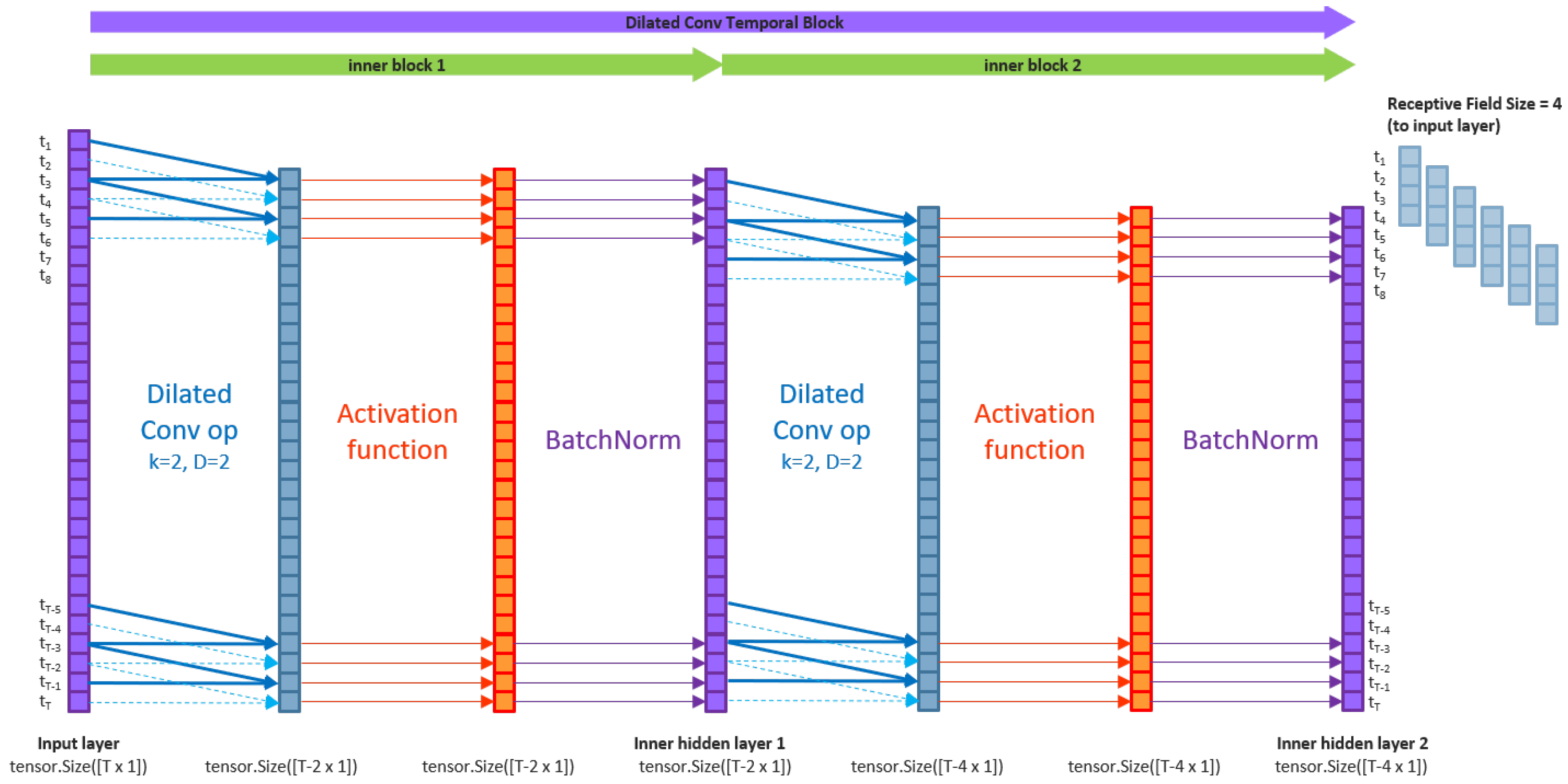
5.1.1. Temporal Convolutional Networks

Temporal convolutional networks (TCNs) are deep convolutional networks that use ‘dilated’ kernels (i.e., kernels that skip nodes in input or hidden layer tensors) in their convolution operations. A dilated kernel of dilation D and kernel size K inserts ‘gaps’ [63] of size $D-1$ between each of the K kernel nodes for convolution. Figure 3 below shows two examples of dilated convolutional operations. Both are dilated kernels of kernel size $K=2$ and convolved with stride $s=1$. The left shows a kernel of dilation $D=1$ over an input time series of size $T\in \mathbb{N}$ reducing the layer output to size $T-1$. The right shows a kernel of dilation $D=2$, reducing the layer output to size $T-2$. Dilated convolution operations are autoregressive.

Figure 3. Dilated convolutional layers. Left: k = 2, s = 1, D = 1. Right: k = 2, s = 1, D = 2.

A TCN $f(X\in {\mathbb{R}}^{N_0\times T_0};L,K,D,\theta )$, parameterised by $\theta$, consists of L hidden layers referred to as temporal blocks, which are composites of element-wise activation functions $\varphi$ and dilated convolution operations of dilation D and kernel size K. The input datum X is an $N_0$-variate tensor of time sequence length $T_0$. At layer $l\in L$ in the TCN, the input and output dimensions will be denoted $X^{l-1}\in {\mathbb{R}}^{N_{l-1}\times T_{l-1}}$ and $X^l\in {\mathbb{R}}^{N_l\times T_l}$, respectively.

Each temporal block for layer l, ${\psi }_l$ contains an element-wise activation function $\varphi$ applied after a dilated convolution operation. The basic temporal block contains an affine operation that convolves some kernel $W_{*D}^{\left(l\right)}$ of size K and dilation factor D striding over the input nodes $X^{l-1}$. This is said to be a dilated convolution of factor D. Kernel strides are convolved along the discrete-time dimension $t\in T,T\in \mathbb{N}$.

Figure 4 below demonstrates the application of the dilated convolution operation on input matrix $X\in {\mathbb{R}}^{N_{l-1}\times T_{l-1}}$ for $K=2,D=2$, and unit stride. This produces an activation tensor $A\in {\mathbb{R}}^{N_l\times T_l}$ where the time dimension $T_l=T_{l-1}-D(K-1)$ before element-wise activation function $\varphi$ is applied.

Figure 4. A dilated convolutional layer applied to a matrix X of data dimension 1. A dilated convolution operation is applied followed by an activation $\varphi$.

Figure 5 shows that temporal blocks may also contain stacks of ‘inner blocks’, each consisting of dilated convolution layers and activations.

Figure 5. An example of temporal block ${\psi }_l$ with two inner blocks of dilated convolutional layers with $k=2,D=2$. An example of topology implemented by Wiese et al. [12] that also included a batch normalisation [64] applied to the output of each activation layer.

Indeed, time series index $t\in \mathbb{N}$ of the output from a dilated convolution operation only incorporates the input from the receptive field of past time series indices $(t-s),s\ge 0,s\le t,s\in \mathbb{N}$. This yields a receptive field size (RFS) of $s+1$, inclusive of endpoints. Thus, only past information is propagated through the TCN network to learn time-lagged feature representations at different scale resolutions.

In the special case where the kernel size is constant for all TCN layers, l, and the dilation factor $D\ge 2$ at layer l is given by $D_l=D^l$, then the TCN is said to be a vanilla TCN.

Finally, the TCN network can include skip layers such as those used in the ResNet [47] architecture to mitigate vanishing gradient problems in learning through deep neural architectures. Figure 6 below explains the topology.

Figure 6. An example of deep temporal convolutional network such as that implemented by Wiese et al. [12]. The topology is L layers of temporal blocks, each with two inner blocks. Weight normalisation [65] is applied to all dilated convolutional operations. Skip connections [47] mitigate vanishing gradient problems for deep networks and enable gradient learning for each latent layer.

The skip temporal block layer ${\eta }_l$ transforms the input $X^{l-1}$ to an output $H_l$ that is accumulated to the final layer L such that:

$$Y=f(X;N_0,N_{L+1},K,B,D,\theta )=\sum _{l=1}^L{H}_l=\sum _{l=1}^L{\eta }_l\left(X^{l-1}\right)$$

(8)

where parameters for the skip layers ${\theta }_{{\eta }_l},l=\{L,L-1,\dots 1\}$ are found through recursion.

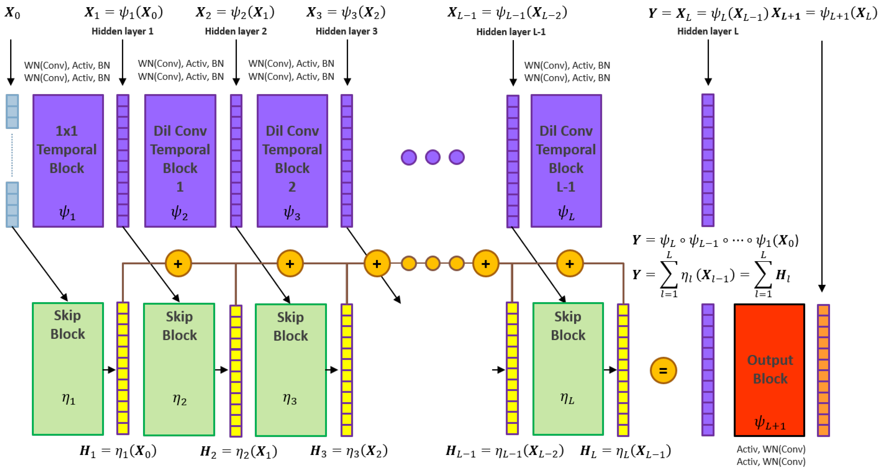
5.1.2. From TCN to Quant GAN

Quant GAN [12] is a generator TCN trained against a discriminator TCN. Detailed descriptions of the TCN, the Quant GAN model, and its training algorithm are provided in Appendix A.1, Appendix A.2 and Appendix A.3.

5.1.3. RSQGAN

RSQGAN is a conditional Quant GAN where conditional class labels correspond to ‘regimes’ of contiguous, non-overlapping time periods. Prior to training RSQGAN, regimes with defined structural breakpoints need to be identified and onehot encoded in preprocessing.

An approach to discovering the time indices ${\left\{{\tau }_j\right\}}_{j=1}^J$ to partition the input data is greedy Gaussian segmentation (GGS) [20]. This approach was chosen for preprocessing because it has a low time complexity and scales well with increasing dimensions $N_X$ and T.

Let $X\in {\mathbb{R}}^{N_X\times T},N_X,T\in \mathbb{N}$ be $N_X$-variate daily log-return time series data. Then, let ${\left\{X_t\right\}}_{t=0}^T$ be the t-indexed returns. Then, let ${\left\{{\tau }_j\right\}}_{j=0}^J,J\in \mathbb{N}$ be structural breakpoints that partition the time series ${\left\{X_t\right\}}_{t=0}^T$ into $J\in \mathbb{N}$ contiguous time periods of class label ${\mathcal{C}}_j$ such that ${\mathcal{C}}_j$ refers to ${\left\{X_t\right\}}_{t={\tau }_{j-1}}^{{\tau }_j},{\tau }_0=0,{\tau }_J=T$.

The J regimes can be used for cGAN training.

5.1.4. RSQGAN Model

RSQGAN is a cGAN learned by training a conditional generator TCN against a conditional discriminator TCN.

Let $J\in \mathbb{N}$ be the number of conditional class regimes for generation, $o_j\in {\mathbb{R}}^J$ be the onehot encoding vector for classes $j=1,\dots ,J$, and let ${\theta }_{E_d}$ and ${\theta }_{E_g}$ be learnable parameters for embedding weight tensors $E_d,E_g$.

Embedding weight tensors $E_d,E_g$ map onehot encodings $o_j$ to class embedding vectors $e_d,\in {\mathbb{R}}^{N_{e_d}},e_g\in {\mathbb{R}}^{N_{e_g}}$ as learnable class embeddings for the conditional discriminator and generator TCNs:

$$E_d:{\mathbb{R}}^J\to {\mathbb{R}}^{N_{E_d}};E_d(o_j;{\theta }_{E_d})\mapsto e_d$$

(9)

$$E_g:{\mathbb{R}}^J\to {\mathbb{R}}^{N_{E_g}};E_g(o_j;{\theta }_{E_g})\mapsto e_g$$

(10)

$cD$ and $cG$ are conditional discriminator and generator networks defined as follows:

$$cD:{\mathbb{R}}^{N_X\times T_{RFS\left(cD\right)}\times J}\to \mathbb{R};cD\left(X\right|{\mathcal{C}}_j)=cD\left(X\right|o_j,{\theta }_{E_d},{\theta }_d)\mapsto \left[0,1\right]$$

(11)

$$cG:{\mathbb{R}}^{N_Z\times T_{\left(RFS\right(cG)+RFS(cD)-1)}\times J}\to {\mathbb{R}}^{N_X\times T_{RFS\left(cD\right)}\times J};cG\left(Z\right|{\mathcal{C}}_j)=cG\left(Z\right|o_j,{\theta }_{E_g},{\theta }_g)\mapsto \tilde{X}|{\mathcal{C}}_j$$

(12)

where $N_X,N_Z$ are the dimensions of the input data and noise prior distributions; the input data distribution is an $N_X$-variate time series of RFS length $T_{RFS\left(cD\right)}$; the noise prior distribution is an $N_Z$-variate time series of RFS length $T_{\left(RFS\right(cG)+RFS(cD)-1)}$; the receptive field sizes of the conditional discriminator and generator are $T_{RFS\left(cD\right)}$ and $T_{RFS\left(cG\right)}$.

The required time dimension of the noise prior used as an input into $cG$ is $T_{\left(RFS\right(cG)+RFS(cD)-1)}$ so that the output of synthetic data $\tilde{X}|{\mathcal{C}}_j$ is of time dimensionality $T_{RFS\left(cD\right)}$ for discriminator evaluation.

The aim is to determine conditional generator ${\theta }_g$ and class embedding ${\theta }_{E_g}$ parameters such that ${\mathbb{P}}_g|{\mathcal{C}}_j={\mathbb{P}}_r|{\mathcal{C}}_j,\forall j=1,\dots ,J$, i.e., $\tilde{X}|{\mathcal{C}}_j\sim {\mathbb{P}}_g|{\mathcal{C}}_j,X|{\mathcal{C}}_j\sim {\mathbb{P}}_r|{\mathcal{C}}_j$, and that

$$cG\left(Z|{\mathcal{C}}_j;p_Z\left(z\right),{\theta }_{E_g},{\theta }_g\right)=p_{X|{\mathcal{C}}_j}(x,o_j)={\mathbb{P}}_r|{\mathcal{C}}_j$$

(13)

Parameters for ${\theta }_g,{\theta }_{E_g}$ can be learned through an alternating optimisation of generator and discriminator loss functions:

$$\underset{{\theta }_g,{\theta }_{E_g}}{min}{\mathbb{E}}_j\mathbb{E}\left[log\left(1-D_{{\widehat{\theta }}_d,{\widehat{\theta }}_{E_d}}\left(G_{{\theta }_g,{\theta }_{E_g}}\left(Z\right|{\mathcal{C}}_j)\right)\right)\right]$$

(14)

$$\underset{{\theta }_d,{\theta }_{E_d}}{max}{\mathbb{E}}_j\mathbb{E}\left[log{D}_{{\theta }_d,{\theta }_{E_d}}\left(X|{\mathcal{C}}_j\right)\right]+\mathbb{E}\left[log\left(1-D_{{\theta }_d,{\theta }_{E_d}}\left(G_{{\widehat{\theta }}_g,{\widehat{\theta }}_{E_g}}\left(Z\right|{\mathcal{C}}_j)\right)\right)\right]$$

(15)

This is equivalent to optimising the conditional vanilla GAN adversarial loss analogous to an unconditional vanilla GAN [6]:

$$\underset{{\theta }_g,{\theta }_{E_g}}{min}\underset{{\theta }_d,{\theta }_{E_d}}{max}{\mathbb{E}}_j\mathbb{E}\left[log{D}_{{\theta }_d,{\theta }_{E_d}}\left(X|{\mathcal{C}}_j\right)\right]+{\mathbb{E}}_j\mathbb{E}\left[log\left(1-D_{{\theta }_d,{\theta }_{E_d}}\left(G_{{\theta }_g,{\theta }_{E_g}}\left(Z\right|{\mathcal{C}}_j)\right)\right)\right]$$

(16)

Expectations are estimated by sampling a minibatch of size $M\in \mathbb{N}$ for all classes $j\in j=1,\dots ,J$.

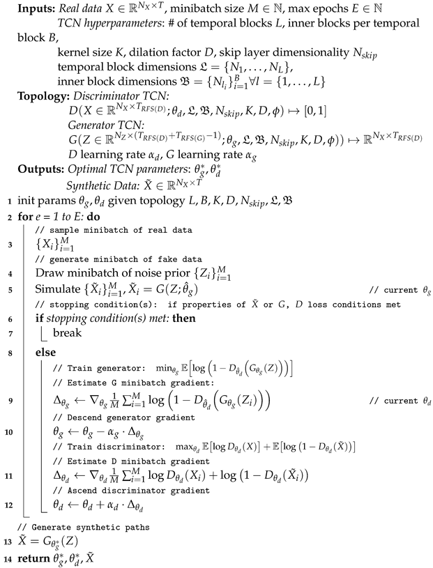
5.1.5. RSQGAN Training Procedure

The RSQGAN training procedure (Algorithm 1) extends the QGAN training procedure (see Appendix A.3) to the conditional case, as shown in Figure 7 below. This only involves minibatch sampling over all regime classes J and updating the class embedding parameters ${\theta }_{E_g},{\theta }_{E_d}$.

Figure 7. The training procedure for RSQGAN. Class regimes ${\mathcal{C}}_j,j\in J$ are input as onehot encoded vectors $o_j$. Embeddings ${\theta }_{E_g},{\theta }_{E_d}$ and network parameters ${\theta }_g,{\theta }_d$ are learned through training. The RSQGAN implementation concatenates the embedded representations $e_d,e_g$ with inputs in the first hidden layer and a fully connected network before forward propagation. This is a similar approach to Brock et al. [21] in the BigGAN architecture to allow for the generation of synthetic data of arbitrary size in the image domain. Adversarial training between $cD(X;{\theta }_d,{\theta }_{E_d})$ and $cG(Z;{\theta }_g,{\theta }_{E_g})$ continues until maximum epochs or stops early if synthetic data $\tilde{X}|{\mathcal{C}}_j$ meet required synthetic standards in training for all classes $j\in J$, e.g., when minibatch average test error metrics fall below certain thresholds.

The base RSQGAN implementation applies the class-conditional encoding $o_j$ for class ${\mathcal{C}}_j$ into the conditional TCN by a learnable embedding representation $e_j$ as an input into the second temporal block. This is a simplification to the ‘z-skip layer’ technique by Brock et al. [21], which suggested a joint noise and class encoding input at each hidden layer of the network. The effect of simplification is to allow for arbitrary size. Testing the efficacy of ‘z-skip layers’ at different time resolutions is expected to further improve the RSQGAN performance and is an area of future work.

Finally, during training experiments, cosine annealing of the learning rate [66] with a periodicity of eight epochs was implemented using the learning rate scheduler in pytorch.

Algorithm 1: RSQGAN training

5.2. Data

Data were collected using a Bloomberg Professional service and data license. Special permission was granted to store data locally for the purposes of this research paper.

At the latest time of data retrieval on 1 July 2020, the maximum daily time series history available for relevant Australian listed stocks was between 4 January 2000 and 30 June 2020 (5346 trading days). Price data were requested, preprocessed, and retrieved using BQL (Bloomberg Query Language) via MS Excel API.

Relevant Australian listed stocks were any stocks that ever attained membership in the top 50% of the market capitalisation of the MSCI Australia market capitalisation weighted index. This represented 19 constituents. There were five stocks that were not continuously listed over this period. These five delisted companies {BXB, FOX, FOXLV, SCG, WFD} were not included. This resulted in a sample universe of 14 Australian stocks {AMP, ANZ, BHP, CBA, CSL, MQG, NAB, QBE, RIO, TLS, WBC, WES, WOW, WPL}.

Stock prices were adjusted for corporate actions (splits and dividends). Stock prices were as at local market close. Where daily data were missing due to public holidays or trading halts, the last available daily closing price was used. All daily stock price time series were then converted to daily log-returns in preprocessing.

5.3. Experimental Design

To select stocks and time periods for designing experimental studies of the RSQGAN versus Quant GAN (QGAN) performance, sub baskets of stocks and time periods were chosen to highlight similarities and differences across the subgroup performance.

To select stocks for training and validation, cross-sectional hierarchical clustering was used to identify stocks from distinct clusters (high intercluster distance) but with near neighbours (close intracluster distance) using the scipy library. Clusters were determined using the complete linkage function under a correlation distance measure.

As expected, the cross-sectional hierarchical clustering of stocks over long time periods clustered into four easily identifiable subgroups: (1) Financials {CBA, WBC, ANZ, NAB, MQG, AMP}, (2) Resources {BHP, RIO, WPL}, (3) Acylicals {WOW, WES, TLS, CSL}, and (4) Globally exposed {QBE}—more similar to Financials and Commodities but less similar to Acyclicals.

Within three clusters with more than one member, the most closely related stocks were {WOW, WES}, {BHP, RIO} and {WBC, ANZ}. The dendrogram in Figure 8 below shows that the training set consists of stocks across each of these clusters: {WOW, BHP, WBC}. The validation set consists of their closest intra-cluster neighbours: {WES, RIO, ANZ}.

Figure 8. Cross-sectional hierarchical stock clusters by log-return correlation of selected Australian Equity stocks in the largest 50% of market cap and complete histories between 4 January 2000 and 30 June 2020. Training set: WOW, BHP, WBC. Corresponding validation set: WES, RIO, ANZ.

To identify time periods that could maximise contrast in generated data between normal and crisis environments, the full-time period was optimally segmented using the GGS algorithm [20].

The GGS algorithm found structural breakpoints that maximise the likelihood that the multivariate daily long returns data across all 14 Australian stocks can be explained by different i.i.d multivariate Gaussian distributions marked by these breakpoints. Key hyperparameters such as the optimal number of breakpoints to use and a regularisation hyperparameter $\lambda$ were found by grid search in 10-fold cross-validation. The open-source Python library ggs [20] was adapted for use for this project.

When GGS was applied ‘globally’ over the full-time period, this resulted in nine distinct regimes. The left chart in Figure 9 shows regime separation by vertical blue lines. The right chart shows the hierarchical clustering of regime similarity using pairwise Wasserstein-2 distances.

Figure 9. Left: GGS is used to segment multivariate daily log-returns optimally into 9 regimes. Right: Wasserstein-2 distance is used to determine a hierarchy of similarity between disjoint contiguous market regimes. Regimes 3, 8 are identified as ‘crisis’ regimes. ‘Non-crisis’ regimes 2, 4, 5, 6, 7 are remarkably similar to each other but dissimilar to pre-2003 and crisis regimes.

As expected, crisis regimes were discovered, such as the ‘GFC crisis regime’ (between 8 November 2007 and 26 August 2009) and the ‘COVID-19 crisis regime’ (from 28 February 2020 to 30 June 2020). These crisis regimes were more similar to each other but most dissimilar to all other regimes. Pre-2003 regimes (5 January 2000–4 September 2003) were notably dissimilar to everything that has been seen since. Five distinct regimes {2, 4, 5, 6, 7} were remarkably similar to each other in the post-2003 pre-COVID era but dissimilar to other regimes.

A ‘study period’ was chosen from the beginning of regime 2 (4 September 2003) until the end of regime 7 (28 February 2020). There was an insufficient length of training data in regime 8 (1 March 2020–30 June 2020) to train a sufficiently high-capacity RSQGAN for that regime.

Figure 10 below shows that long-term average correlation behaviour does not hold specifically for the given regimes. This suggests that not conditionally accounting for distinct regime modes may degrade the performance of unconditional models.

Figure 10. Left: Long-term log-return correlation distances. Right: Correlation heatmap for each of the 9 regimes. GFC regime—2nd row, 1st column; COVID-19 regime—3rd row, 3rd column.

Multivariate daily log-returns for the training set {WOW, BHP, WBC} in the study period were then ‘locally’ segmented by forcing two breakpoints (three regimes) using the GGS algorithm again. This is shown in Figure 11 below. Forcing two breakpoints to be discovered led to dates being recalibrated for the three distinct regimes: (1) a ‘normal’ pre-GFC regime (4 September 2003—9 January 2008); (2) a ‘crisis’ GFC regime (9 January 2008—9 June 2009); and (3) a ‘normal’ post-GFC, pre-COVID regime (9 June 2009–28 February 2020).

Figure 11. GGS is applied again locally to segment multivariate daily log-returns for only the study stocks WOW, BHP, and WBC. To form the study, the crisis regime was separated from normal regimes by forcing two breakpoints. Blue lines mark dates where structural breakpoints were optimally set. Left: historical stock prices for study stocks. Right: daily log-return scatter plots for study stocks.

The separate validation stock set {WES, RIO, ANZ} was not locally segmented using the GGS algorithm [20] as breakpoint dates found through GGS may not be identical to the study set. For validation stocks, the same breakpoints discovered through GGS on the training set were enforced, as the timing for regimes should be consistent across the market. The local application of GGS to discover breakpoints did not include validation stocks, so that information leakage from the behaviour of validation stocks would not influence the position of training set breakpoints.

5.4. Evaluation by Stylised Facts

For this report, the performance of the proposed conditional RSQGAN is compared to the unconditional QGAN performance, keeping the topology and training hyperparameters constant.

Denote $r_{i,t}$ as the log-return for asset i over time period $(t-1,t)$ given by $r_{i,t}:=log{S}_{i,t}-log{S}_{i,t-1}$, where $S_{i,t}$ is the price of asset $i=\{1,\dots ,N\}$ at time $t=\{0,\dots ,T\}$.

Table 1 summarises common univariate stylised facts (SFs) used and cited by Takahashi et al. [11], Wiese et al. [12]. The original source papers for these SFs are in the right column. Loss metrics used to evaluate the RSQGAN and QGAN performance are based on the mean absolute difference of synthetic data versus the real data for various SF metrics.

Table 1. Description of stylised facts.

Stylised Fact (SF)	Evaluation Metric
1. Linear unpredictability	$Corr(r_t,r_{t+k})=\frac{\mathbb{E}\left[(r_t-{\mu }_r)(r_{t+k}-{\mu }_r)\right]}{\widehat{{\sigma }_r^2}}$ $Corr(r_t,r_{t+k})\approx 0,k\ge 1$
2. Heavy-tailed distribution	$f_R\left(r\right)\propto r^{-\alpha }$ $f_R\left(r\right)$ is the p.d.f of R, $\alpha \in [3,5]$
3. Volatility clustering	$Corr\left(\right|r_t|,|r_{t+k}\left|\right)\propto k^{-\beta }$ up to large k, small $\beta$
4. Leverage effect	$L\left(k\right)=\frac{\mathbb{E}\left[r_t|r_{t+k}{|}^2-r_t{\left|r_t\right|}^2\right]}{\mathbb{E}{\left[|r_t^2|\right]}^2}$ $L\left(k\right)<0$ for $k\in [1,10]$
5. Coarse–fine vol correlation	$\Delta {\rho }_{cf}^{\tau }\left(k\right)={\rho }_{cf}^{\tau }\left(k\right)-{\rho }_{cf}^{\tau }(-k)$ ${\rho }_{cf}^{\tau }\left(k\right)=Corr\left(|{\sum }_{i=1}^{\tau }{r}_{t+k-i}|,{\sum }_{i=1}^{\tau }\left|r_{t-i}\right|\right)$ for some $k>0$ $\Delta {\rho }_{cf}^{\tau }\left(k\right)<0$
6. Gain/loss asymmetry	$T_{wait}^t\left(\theta \right)$ = $\left\{\begin{array}{c}{inf}_{t^{\prime }}{r}_{t+t^{\prime }}\ge \theta ,\theta >0\hfill \\ {inf}_{t^{\prime }}{r}_{t+t^{\prime }}\le \theta ,\theta <0\hfill \end{array}\right.$

A summary of properties of SFs 1–6 was provided by Takahashi et al. [11].

• Linear unpredictability [43] refers to the rapid decay of return autocorrelations even over small time lags, which reflects some evidence of market efficiency. This is captured by examining the autocorrelation function (ACF) of returns up to some maximum time lag.
• Heavy-tailed return distribution [43,53] refers to the phenomenon where the return distribution density fits a power, rather than exponential, law function. There is a tendency for very large positive returns for some stocks, which manifest as excess return kurtosis relative to a Gaussian distribution.
• Volatility clustering [42] refers to the phenomenon where periods of high volatility (temporal standard deviation of returns) tend to be autocorrelated with periods of high volatility. This can be observed by fitting the ACF of absolute log-returns to a power-law function with low decay parameter $\beta$.
• Leverage effect [54,55] refers to the observation that past price returns are negatively correlated with future volatility. It could be observed that the numerator of the lead-lag correlation expression $L\left(k\right)$, given by $\mathbb{E}\left[r_t|r_{t+k}{|}^2-r_t{\left|r_t\right|}^2\right]$, is negative if, for $r_t<0$, $|r_{t+k}{|}^2-{\left|r_t\right|}^2>0$, i.e., negative returns predict higher future volatility (and, vice-versa, that positive returns predict lower future volatility).
• Coarse–fine volatility correlation [56,57,58] is a measure of the correlation of the volatility structure observed over a historical period $\tau$ when looking at two different time resolutions. The lower-resolution volatility, coarse volatility, given by $|{\sum }_{i=1}^{\tau }{r}_{t-i}|$, measures the absolute historical returns between time $(t-\tau ,t)$. The fine volatility, measured by ${\sum }_{i=1}^{\tau }\left|r_{t-i}\right|$, is a measure of the absolute daily return variations between time $(t-\tau ,t)$. The coarse–fine volatility with lag k, ${\rho }_{cf}^{\tau }\left(k\right)=Corr\left(|{\sum }_{i=1}^{\tau }{r}_{t+k-i}|,{\sum }_{i=1}^{\tau }\left|r_{t-i}\right|\right)$, measures the time dependency between fine and k-lagged coarse volatility. The lead lag correlation given by $\Delta {\rho }_{cf}^{\tau }\left(k\right)={\rho }_{cf}^{\tau }\left(k\right)-{\rho }_{cf}^{\tau }(-k)$ would indicate if a higher historical lead-lag correlation is predictive of a lower lead-lag correlation in the future—a kind of regime-switching behaviour as measured by coarse and fine volatility at total lag $2k$.
• Gain/loss asymmetry [59] is the phenomenon where positive total returns take a longer time to accrue than negative absolute returns. In other words, the speed at which return drawdowns occur tends to be faster than the speed at which return accumulation occurs. This is measured by observing the empirical distribution of wait time random variable $T_{wait}^t\left(\theta \right)$ for upper and lower return threshold (barriers) $\pm \theta$ to be struck.

5.5. Hardware and Software

Only limited local resources were required to carry out this research due to the relatively low dimensionality of FTS data compared to other data domains (e.g., text, images, video). Further, the use of dilated kernels in QGAN and RSQGAN TCN architectures is efficient in terms of the number of parameters needed to cover a large effective receptive field size [63], enabling training to take place on a local GPU within a reasonable length of time.

The local hardware resources used were: i7-8750H @ 2.20 GHz, 16 Gb RAM, NVIDIA GTX 1060 GPU.

The key packages used were Python 3.7.7, Pytorch 1.4.0, Plotly 4.9.0, ggs [20], and stylefact [11].

6. Results

The performance was compared between a single RSQGAN model and multiple QGANs each trained on data from a single regime. This is a stringent benchmark test for RSQGAN as it competes against multiple QGAN models. The topology and training hyperparameters were varied but held constant between the two models, so the effect of regime conditional embedding and z-clipping hyperparameters could be observed in isolation.

The results suggest that RSQGAN could generate crisis regime synthetic data better than a QGAN trained only on crisis regime data. RSQGAN appears to benefit from both categorical class encoding and parameter sharing across a single network to benefit the minority ‘crisis’ regime (at the expense of a poorer performance in the majority ‘non-crisis’ regime).

6.1. Evaluation Metrics

The open-source stylefact library implemented by Takahashi et al. [11] was used and adapted to compare and evaluate the performance of RSQGAN versus QGAN.

Definitions for SF test metrics used to evaluate and compare the QGAN and RSQGAN performance are shown in Table 2 below.

Table 2. Stylised fact (SF) test losses.

SF Test Losses	Interpretation and Sources	Expression
acf	ST unpredictability Chakraborti et al. [43]	${\sum }_k|{\widehat{\gamma }}_R\left(k\right)-\frac{1}{M}{\sum }_{i=1}^M{\widehat{\gamma }}_{G_i}\left(k\right)|$ $\gamma \left(k\right)=\rho (r_t,r_{t+k}),k\in \mathbb{N}$
pdf	Return density Chakraborti et al. [43] Liu et al. [53]	$\int \parallel {\widehat{f}}_R\left(r\right)-\frac{1}{M}{\sum }_{i=1}^M{\widehat{f}}_{G_i}\left(r\right)\parallel dr$
vc_acf*	Volatility clustering Cont [42]	${\sum }_k|{\widehat{\nu }}_R\left(k\right)-\frac{1}{M}{\sum }_{i=1}^M{\widehat{\nu }}_{G_i}\left(k\right)|$ $\nu \left(k\right)=\rho \left(\right|r_t|,|r_{t+k}\left|\right),k\in \mathbb{N}$
vc_pdf	Abs. return density Cont [42]	$\int \parallel {\widehat{f}}_R\left(r\right)-\frac{1}{M}{\sum }_{i=1}^M{\widehat{f}}_{G_i}\left(r\right)\parallel dr$
leveff*	Loss future vol lag Bouchaud et al. [54] Qiu et al. [55]	${\sum }_k|{\widehat{L}}_R\left(k\right)-\frac{1}{M}{\sum }_{i=1}^M{\widehat{L}}_{G_i}\left(k\right)|$ $L\left(k\right)=\mathbb{E}\left[r_t|r_{t+k}{|}^2-r_t{\left|r_t\right|}^2\right]/\mathbb{E}{\left[|r_t^2|\right]}^2$
cfvol*	Coarse–fine vol lag Müller et al. [56] Rydberg [57] Gavrishchaka and Ganguli [58]	${\sum }_k|{\widehat{\rho }}_R^{\tau }\left(k\right))-\frac{1}{M}{\sum }_{i=1}^M{\widehat{\rho }}_{G_i}^{\tau }\left(k\right)|$ ${\rho }^{\tau }\left(k\right)=\rho \left(|{\sum }_{i=1}^{\tau }{r}_{t+k-i}|,{\sum }_{i=1}^{\tau }\left|r_{t-i}\right|\right)$
cfvol_diff	Coarse–fine vol skew Müller et al. [56] Rydberg [57] Gavrishchaka and Ganguli [58]	${\sum }_k|{\widehat{\Delta }}_R^{\tau }\left(k\right))-\frac{1}{M}{\sum }_{i=1}^M{\widehat{\Delta }}_{G_i}^{\tau }\left(k\right)|$ ${\Delta }^{\tau }\left(k\right)={\rho }^{\tau }\left(k\right)-{\rho }^{\tau }(-k)$
gain_cdf_$\theta$	Gain stoptime CDF Jensen et al. [59]	${\sum }_t|{\widehat{F}}_{T_R^{gain}}\left(t\right)-\frac{1}{M}{\sum }_{i=1}^M{\widehat{F}}_{T_{G_i}^{gain}}\left(t\right)|$ $T_{gain}^t(t;\theta )={inf}_{t^{\prime }}{r}_{t+t^{\prime }}\ge \theta ,\theta >0$
loss_cdf_$\theta$*	Loss stoptime CDF Jensen et al. [59]	${\sum }_t|{\widehat{F}}_{T_R^{loss}}\left(t\right)-\frac{1}{M}{\sum }_{i=1}^M{\widehat{F}}_{T_{G_i}^{loss}}\left(t\right)|$ $T_{loss}^t(t;\theta )={inf}_{t^{\prime }}{r}_{t+t^{\prime }}\le \theta ,\theta <0$

The model performance is measured for each SF loss metric. An SF loss metric is the mean absolute deviation between the SF metric for real and synthetic data, which are then mean averaged against overall stocks in the training or validation set. SF loss metrics can be used to compare the model performance for each regime but can also be averaged over all regimes to evaluate the general performance. The results are shown for training and validation stock sets.

For crisis risk management applications, the focus should be placed on four SF test metrics marked with asterisks in Table 2: {vc_acf, leveff, cfvol, loss_cdf_$\theta$}. This is because each of these ‘crisis-sensitive’ SF metrics is some measure of time or path-dependent (rather than distributional) behaviour and might be actionable in a real-world crisis scenario. The first three represent the ACF of returns and/or volatility given observations about recent returns and/or volatility. The fourth, loss_cdf_$\theta$, is the cumulative distribution function of stoptimes needed to reach a cumulative loss of $-\theta$ for some $\theta >0$. Knowledge of this distribution could help risk managers determine a time-duration-sensitive portfolio management strategy.

6.2. Key Results

The results indicate that RSQGAN learned a single joint representation of FTS behaviour over multiple regimes that is consistent with the performance of multiple QGAN representations each trained on data only from a single regime. RSQGAN outperformed QGAN for the minority ‘crisis’ regime class. Though RSQGAN SF test metrics in crisis environments show some improvement compared to QGAN trained only on ‘crisis’ data, it is not desirable to seek SF scores as close to zero as possible, which would indicate mode collapse.

Table 3 and Table 4 show the performance of RSQGAN versus QGAN across the range of SF test losses averaged over training stocks {WOW, BHP, WBC} and validation stocks {WES, RIO, ANZ}, respectively. In the first column, the SF test loss is bolded only if RSQGAN outperformed QGAN (lower is better). The second column shows in bold the outperforming model on that SF test loss. The third column shows the SF test loss averaged over all regimes for information purposes only. SF test losses are bolded for the crisis regime as the main class of interest.

Table 3. Single RSQGAN vs. multiple QGANs trained on single regime data. Training set. Hidden layer topology: 6 hidden layers and skip layers of 50 nodes each. Cosine annealing. $z^{clip}=2.5$ (train), $z^{clip}=2.3$ (generation).

		All Regimes	Crisis Regime
acf	rsqgan	2.135	2.757
	qgan	2.030	3.197
pdf	rsqgan	0.641	0.770
	qgan	0.588	0.671
vc_acf*	rsqgan	2.351	3.213
	qgan	2.566	3.111
vc_pdf	rsqgan	0.396	0.479
	qgan	0.347	0.502
leveff*	rsqgan	1924.233	1463.868
	qgan	1607.904	1835.097
cfvol*	rsqgan	4.749	6.202
	qgan	5.199	6.327
cfvol_diff	rsqgan	2.430	3.886
	qgan	2.386	3.840
gain_cdf_12_5	rsqgan	21.826	19.622
	qgan	23.052	19.119
loss_cdf_12_5*	rsqgan	24.968	20.450
	qgan	24.259	21.305

Table 4. Single RSQGAN vs. multiple QGANs trained on single regime data. Validation set. Hidden layer topology: 6 hidden layers and skip layers of 50 nodes each. Cosine annealing. $z^{clip}=2.5$ (train), $z^{clip}=2.3$ (generation).

		All Regimes	Crisis Regime
acf	rsqgan	1.824	2.619
	qgan	1.779	2.723
pdf	rsqgan	0.826	0.953
	qgan	0.712	0.838
vc_acf*	rsqgan	2.548	3.619
	qgan	2.794	3.685
vc_pdf	rsqgan	0.393	0.582
	qgan	0.375	0.503
leveff*	rsqgan	2091.035	2718.220
	qgan	1726.681	2139.719
cfvol*	rsqgan	4.743	6.181
	qgan	5.086	6.305
cfvol_diff	rsqgan	2.310	3.743
	qgan	2.311	3.735
gain_cdf_12_5	rsqgan	24.841	13.825
	qgan	24.338	12.592
loss_cdf_12_5*	rsqgan	31.333	15.159
	qgan	32.698	16.431

The key results demonstrated shown in this section suggest a choice of topology and training hyperparameters that may generalise well out of sample. Some other topological and training hyperparameter choices experimented on resulted in an extremely strong performance on the training stock set but relatively weaker results on the validation stock set.

However, some caution should be exercised when interpreting these results:

• Minimising crisis regime SF test losses toward zero is not desired.
  This outcome may be indicative of mode collapse. GANs are susceptible to mode collapse for reasons described in Section 2. High intra-class entropy (variability) is desirable and is a measure of GAN quality. The purpose of RSQGAN in risk management applications is to provide a rich, non-degenerate synthetic density distribution. Hence, hyperparameter choices should focus on the relative improvement over QGAN without aiming to drive crisis regime SF test losses to zero. An equivalent metric for Fréchet joint distance [40] in the image domain that balances fidelity versus variety does not yet exist for the FTS domain. The investigation will be left for future work.
• GAN training is notoriously unstable, leading to performance variations sensitive to the number of training epochs.
  SF test losses can be unstable due to the instability of learned generator representations during training. Potential approaches to dealing with this were discussed in Section 3.1. Hence, the results shown in these tables do not include RSQGAN improvements that could be captured through the use of improved GAN objective loss functions or research into the calibration of early stopping criteria. This has been left for future work.

Synthetic output samples for training and validation stocks are shown in Figure 12 and Figure 13 below.

Figure 12. Real versus synthetic stock price paths generated by QGAN and RSQGAN by stock and regime. Subplot rows: stocks WOW, BHP, and WBC, respectively. Subplot columns: regimes 0, 1, and 2, respectively. Regime ‘1’ is the crisis regime. Purple paths: 128 synthetic QGAN paths trained only on single-regime class data. Orange paths: 128 synthetic RSQGAN paths generated for each regime and a given stock from a single conditional GAN model. Black line: real stock price history.

Figure 13. Real versus synthetic stock price paths generated by QGAN and RSQGAN by stock and regime. Subplot rows: stocks WES, RIO, and ANZ, respectively. Subplot columns: regimes 0, 1, and 2, respectively. Regime ‘1’ is the crisis regime. Purple paths: 128 synthetic QGAN paths trained only on single-regime class data. Orange paths: 128 synthetic RSQGAN paths generated for each regime and a given stock from a single conditional GAN model. Black line: real stock price history.

Figure 14 and Figure 15 show the quality of RSQGAN and QGAN fit to ‘crisis-sensitive’ SF test metrics. Black, orange, and blue traces correspond to real, RSQGAN synthetic, and QGAN synthetic SF test metrics, respectively.

Figure 14. SF training losses by QGAN and RSQGAN by stock in crisis regime training over 256 epochs. In-sample stocks. Subplot order: WOW, BHP, and WBC. Top left panel: Volatility clustering ACF. Top right panel: Leverage effect. Bottom left: Coarse–fine volatility. Blue dots/traces: QGAN SF test metrics. Orange dots/traces: RSQGAN SF test metrics. Black dots/traces: Real data. Bottom right: Cumulative loss stoptime for $\theta =12.5$. Darkbrown trace: Real stoptime CDF. Gray traces: QGAN. Red traces: RSQGAN. Note that RSQGAN is simultaneously training on two other regimes.

Figure 15. SF training losses by QGAN and RSQGAN by stock in crisis regime training over 256 epochs. Validation stocks. Subplot order: WES, RIO, and ANZ. Top left panel: Volatility clustering ACF. Top right panel: Leverage effect. Bottom left: Coarse–fine volatility. Blue dots/traces: QGAN SF test metrics. Orange dots/traces: RSQGAN SF test metrics. Black dots/traces: Real data. Bottom right: Cumulative loss stoptime for $\theta =12.5$. Darkbrown trace: Real stoptime CDF. Gray traces: QGAN. Red traces: RSQGAN. Note that RSQGAN is simultaneously training on two other regimes.

7. Discussion

Various experiments were designed to explore how variations in RSQGAN topology and hyperparameter settings may impact its performance versus the QGAN benchmark. The general observations that could be made from these experiments were:

• The QGAN and RSQGAN performance can be highly variable between assets and regimes for fixed topology and hyperparameter settings. The baseline settings used were the same architectural and hyperparameter settings as the QGAN open-source implementation by Wiese et al. [12]. Unsurprisingly, these settings resulted in a mixed performance across all stocks and regimes. Baseline QGAN settings consisted of six hidden layers and skip layer connections of 50 nodes each while using fixed discriminator and generator learning rates of $0.0003$ and $0.0001$, respectively. On the training stock set, RSQGAN outperformed QGAN on all four crisis-sensitive SF test metrics. However, on the validation stock set, RSQGAN only outperformed on the loss CDF stoptime distribution. By construction, the conditional RSQGAN, which is trained by learning from average class losses, performs similarly to the average of multiple QGANs each trained on single-regime datasets. But due to regime class imbalance, it outperforms the minority crisis regime class at the expense of the performance on the ‘normal’ regime classes. However, as the performance was observed to be highly variable across stock and regime conditions, this suggests that additional model flexibility is required to deal with different regime lengths or stock-specific behaviour. Choosing an appropriate receptive field size (and hence network depth) is an important hyperparameter for simulating different regime lengths in a single model. Selecting an RFS that is too short could lead to longer-term time independence in simulations than is justifiable. Selecting an RFS that is too long would reduce the effective training dataset while increasing learnable parameters. The receptive field size should be consistent with the intended simulation horizon. Despite selecting training and validation stock sets from the same long-term correlation cluster, the mixed performance between stocks and regimes highlights that the same RSQGAN topology was not sufficiently rich to learn stock-specific features that could be applied from one stock (e.g., BHP) and to expect a similarly strong performance in a highly correlated stock (e.g., RIO). Thus, a richer topology such as a joint drift and volatility GAN, such as the stochastic volatility neural network (SVNN) model by Wiese et al. [12], could be extended to the conditional case in the future. A single-drift topology in isolation will underperform in simulating stocks that show strong momentum characteristics (i.e., a negative leverage effect) where high returns predict lower future volatility. An additional approach to potentially learning stock-specific features and improving the RSQGAN performance is to jointly condition regime categorical classes with continuous variables such as rolling volatility, correlation, or recent historical time series such as that demonstrated by Koshiyama et al. [13], de Meer Pardo [14], Fu et al. [15].
• A higher-capacity topology appears to further improve the RSQGAN performance relative to QGAN.
  A larger-capacity RSQGAN/QGAN network with seven hidden layers and skip layer connections of 60 nodes each led to RSQGAN outperforming in nine out of nine SF test metrics for the training stock set. However, RSQGAN outperformed in only two out of nine SF test metrics for the validation stock set. An examination of training losses indicates that this was partially due to training instability, which could be rectified by improved objective loss functions and early stopping criteria. This is left for future investigation. A poor performance on the validation stock set could also be due to the RSQGAN topology not being flexible enough to learn necessary stock-specific features (see the point above).
• The choice of early stopping criteria for training QGAN and RSQGAN is a significant area for further improvement.
  The original early stopping criteria in the open-source implementation by Wiese et al. [12] was used. The early stopping of QGAN and RSQGAN training occurred if the mean absolute deviation of the ACF of log-returns and the ACF of absolute returns both fell below preset thresholds.
  Figure 16 below shows that, during training for a given regime, none of the six possible stopping criteria uniformly converge for any of the three training stocks. This could be due to a number of causes—a topology without the sufficient capacity to simultaneously learn all SF behaviours and/or unstable training. Further, it is not necessarily desirable for convergence over all SF behaviours, as it may suggest mode collapse. No experiments were conducted to explore if there were reliable heuristics for setting early stopping conditions and understanding trade-offs between individual SF test metrics. This remains an open problem and is left for future work.
  

  Figure 16. SF losses by QGAN and RSQGAN by stock for crisis regime training over 256 epochs. Subplot rows: stocks WOW, BHP, and WBC, respectively. Subplot columns: SF training losses for log-return pdf, kurtosis, skewness, ACF of log-returns, ACF of absolute log-returns, leverage effect. Blue dots: QGAN SF training losses. Orange dots: RSQGAN SF training losses. Note that RSQGAN is simultaneously training on two other regimes.
• A modest z-clipping of noise prior to $z^{clip}=2.5$ in training and $z^{clip}=2.3$ in generation appeared to improve the performance further.
  Experiments with a ‘crude’ implementation of z-clipping and skip-z layers from the BigGAN paper by Brock et al. [21] showed that modest z-clipping could produce synthetic data with higher initial fidelity to real data.
  The ‘crude’ RSQGAN implementation only applied skip-z layers to the first hidden layer of the generator and discriminator networks rather than learnable embeddings at all hidden layers. Further, it did not include the authors’ suggestion to implement an orthogonal regularisation of the generator. Despite the crude implementation, modest but mixed performance improvements were observed across SF test losses when a modest z-clipping of $z^{clip}=2.5$ in training and $z^{clip}=2.3$ in generation were applied.
  However, an experiment that used a more extreme clipping parameter $z^{clip}=1.5$ in training and $z^{clip}=1.25$ in generation appeared to degrade the relative performance of RSQGAN relative to QGAN. A full implementation of z-clipping and skip-z layers and further experiments are left to future work.
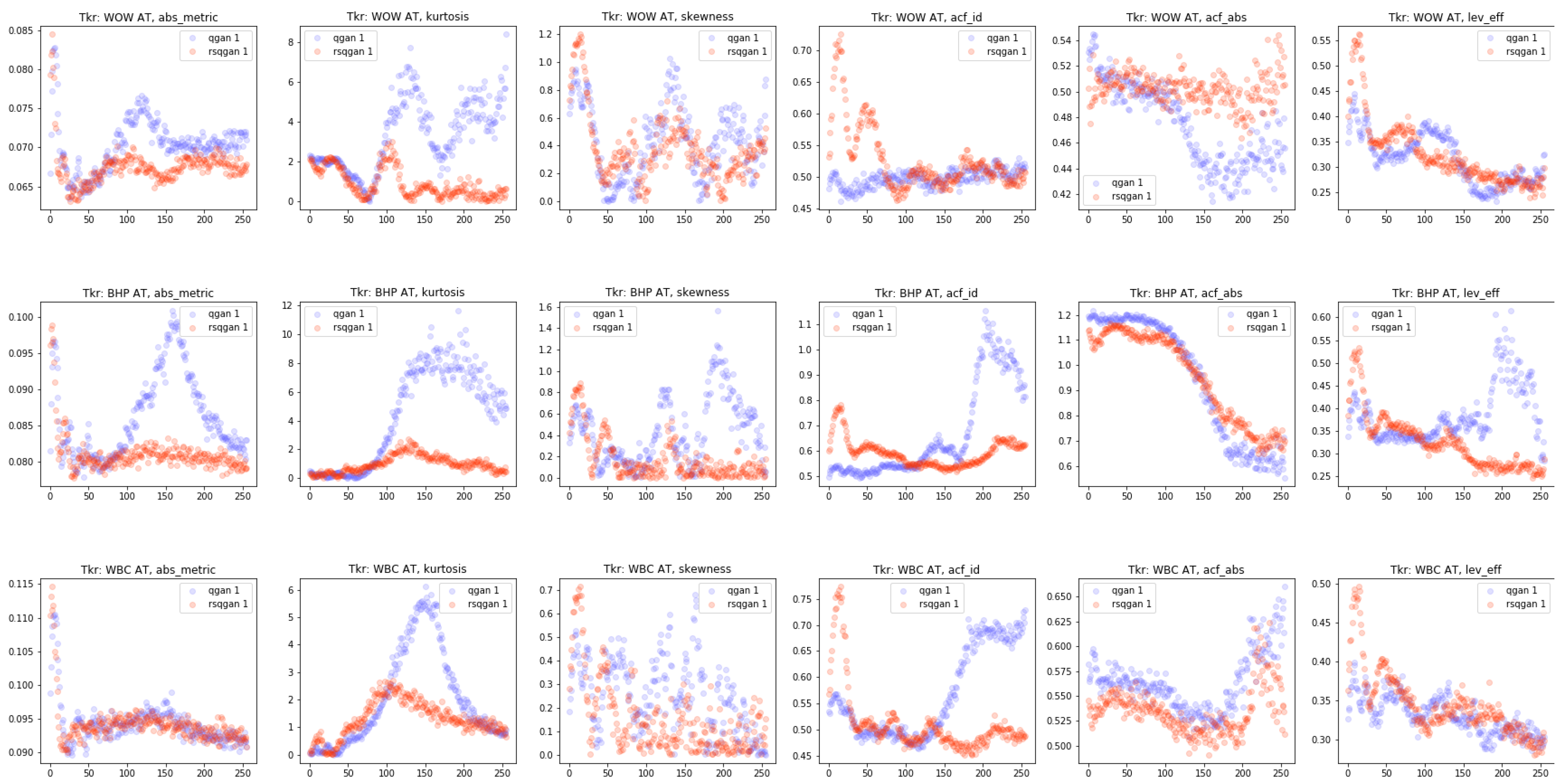
• RSQGAN produced synthetic data from crisis regimes with improved SF evaluation measures.
  It is reasonable to expect an RSQGAN outperformance for the minority crisis regime, as the RSQGAN training procedure corrects for regime class imbalance and enables shared parameter learning across all classes in a single model representation. This is a useful property for crisis risk management applications where fewer historical crisis data are observable.
  Improving simulations for the expected decay of the ACF of absolute returns or volatility could be useful for assessing the value of options instruments. By similar arguments, an improved simulation of expected future volatility based on recent returns or simulating multiperiod (coarse) or intraday (fine) volatility with a lag given observed coarse or fine volatility could assist with risk decision making. Further knowledge of the time distribution for different loss thresholds could assist with a trading strategy. SF test metrics corresponding to these actionable concepts are volatility clustering ACF, leverage effect, coarse–fine volatility lag, and loss stoptime CDF.

8. Future Work

Promising areas for future research to improve RSQGAN model and synthetic data quality include: (1) a richer joint conditioning of regime classes and continuous variables such as volatility or a short historical time series; (2) topological enhancements such as a higher RSQGAN capacity, full implementation of skip-z and z-clipping [21], and joint drift and volatility networks [12]; (3) training and stability improvements such as early stopping experimentation, or using alternative loss functions such as WGAN [34], WGAN-GP [35], or RaGAN [52]; and (4) investigating the relationship between satisfying multiple SFs as indicators of synthetic quality and its potential correlation with a single measure of quality analogous to the Fréchet joint distance [40] in the image domain.

9. Conclusions

For risk management applications, the task of modelling FTS behaviour and densities in crisis regimes is of greater cost-sensitive importance than normal regimes. Though the value at stake is considerably higher during crisis regimes, historical experiences of crisis regimes are sparse.

RSQGAN is a new approach for generating regime-specific synthetic data by extending the unconditional Quant GAN [12]. RSQGAN is a conditional FTS GAN that benefits from learning time-dependent features of minority ‘crisis’ regime classes through class embedding and parameter sharing with majority ‘normal’ regime classes. Initial experiments suggest that RSQGAN appears to perform well in learning crisis regime behavior, even when only using categorical class embedding by labels applied from GGS preprocessing [20].

Though many measures of stylised facts are good for assessing the quality of an FTS GAN, some have larger implications for decision making in a crisis environment because path-dependent behaviour could be acted upon. Four particular evaluation SF test metrics have been identified.

The further development of RSQGAN could provide additional input for making more robust risk management decisions in a time of market crisis.

Appendix A.1. Temporal Convolutional Networks

Temporal convolutional networks (TCNs) are deep convolutional networks that use ‘dilated’ kernels (i.e., kernels that skip nodes in input or hidden layer tensors) in their convolution operations. A dilated kernel of dilation D and kernel size K inserts ‘gaps’ [63] of size $D-1$ between each of the K kernel nodes for convolution. See Figure A1 below.

Figure A1. Dilated convolutional layers. Left: k = 2, s = 1, D = 1. Right: k = 2, s = 1, D = 2.

It is demonstrated below (see Equation (A10)) that kernel dilations increase effective receptive field sizes, which allows TCNs to discover representations for longer-term time dependencies using a relatively lower number of shared parameters.

Appendix A.1.1. Multilayer Perceptron

First, let $f\left(N_0,N_{L+1};\theta \right)$ be a multilayer perceptron (MLP) that is a non-linear mapping of ${\mathbb{R}}^{N_0}\to {\mathbb{R}}^{N_{L+1}}$ over $L\in \mathbb{N}$ hidden layers such that:

$$f(X;X\in {\mathbb{R}}^{N_0},\theta \in \Theta )=a_{L+1}\circ f_L\circ ...\circ f_1\left(X\right)$$

(A1)

where ∘ are function compositions and the affine transformation $a_l$ is given by

$$a_l:{\mathbb{R}}^{N_{l-1}}\to {\mathbb{R}}^{N_l},a_l\left(X_{l-1}\right)=W^{\left(l\right)}{X}_{l-1}+b^{\left(l\right)},\forall l\in L,N_l\in \mathbb{N}$$

(A2)

where each layer l is parameterised by ${\theta }_l=\left(W^l,b^{\left(l\right)}\right)$ and $X_{l-1}$ is the input to layer l.

Each hidden layer l is a non-linear mapping expressed as a composite activation and affine operation:

$$f_l:{\mathbb{R}}^{N_{l-1}}\to {\mathbb{R}}^{N_l},f_l=\varphi \left(a_l\right)$$

(A3)

where $\varphi :\mathbb{R}\to \mathbb{R}$, $\varphi \left(0\right)=0$ is a non-linear, Lipschitz continuous activation function applied element-wise to $a_l$.

Thus, the learnable parameters of the MLP of L hidden layers are $\theta :=\left({\theta }_1,\dots ,{\theta }_{L+1}\right)$.

Appendix A.1.2. TCN Model Definition

Analogous to an MLP $f(X\in {\mathbb{R}}^{N_0};L,\theta )$, a TCN $f(X\in {\mathbb{R}}^{N_0\times T_0};L,K,D,\theta )$ consists of L hidden layers referred to as temporal blocks, which are composites of element-wise activation functions $\varphi$ and dilated convolution operations as explained below. The input datum X is an $N_0$-variate tensor of time sequence length $T_0$.

Each temporal block composite function ${\psi }_l$ contains an element-wise activation function $\varphi$ applied after a convolution operation. The basic temporal block contains an affine operation that convolves some kernel W of size K and dilation factor D striding over the input nodes $X_{l-1}$. This is said to be a dilated convolution of factor D. Kernel strides are convolved along the discrete-time dimension $t\in T,T\in \mathbb{N}$. Temporal blocks may also contain stacks of inner blocks consisting of dilated convolution and activation operations (see Figure A3 below).

The diagram below shows two examples of dilated convolutional operations. Both are dilated kernels of kernel size $K=2$ and convolved with stride $s=1$. The left shows a kernel of dilation $D=1$ over an input time series of size $T\in \mathbb{N}$ reducing the layer output to size $T-1$. The right shows a kernel of dilation $D=2$, reducing the layer output to size $T-2$. Dilated convolution operations are autoregressive.

Let $W_{*D}^{\left(l\right)}$ be a dilated kernel of size K and dilation factor D in some TCN layer l. Then, the output of a dilated convolution operation ${}_{*D}$ [12] applied on $X\in {\mathbb{R}}^{N_{l-1}}\times T_{l-1}$ across input dimension index $m=1,\dots ,N_{l-1}$ yielded at time index $t\le T$ is given by:

$${\left(W_{*D}^{\left(l\right)}X\right)}_{m,t}:=\sum _{i=1}^K\sum _{j=1}^{N^{(l-1)}}{W}_{i,j,m}·X_{j,t-D(K-i)}$$

(A4)

Figure A2 below demonstrates the application of the dilated convolution operation of kernel $W_{*D}$ on input matrix $X\in {\mathbb{R}}^{N_{l-1}\times T_{l-1}}$ applied for $K=2,D=2$, and unit stride. This produces an activation tensor $A\in {\mathbb{R}}^{N_l\times T_l}$ where the time dimension $T_l=T_{l-1}-D(K-1)$ before element-wise activation function $\varphi$ is applied.

Figure A2. A dilated convolutional layer applied to a matrix X of data dimension 1. A dilated convolution operation is applied followed by an activation $\varphi$.

Indeed, time series index $t\in \mathbb{N}$ of the output from a dilated convolution operation only incorporates the input from the receptive field of past time series indices $(t-s),s\ge 0,s\le t,s\in \mathbb{N}$. This yields a receptive field size (RFS) of $s+1$, inclusive of endpoints. Thus, only past information is propagated through the TCN network to learn time-lagged feature representations at different scale resolutions.

A temporal block may contain one or more ‘inner blocks’ of composite activation and dilated convolution layers. Define a temporal block function for layer l, ${\psi }_l$ with parameters $(N_{l-1},N_l,S_l)$. It contains an arbitrary number of inner blocks $i,i\in \mathbb{N}$ and own parameters $(N_{l_{i-1}},N_{l_i},S_{l_i})$ such that the temporal block is a mapping:

$${\psi }_l:{\mathbb{R}}^{N_{l-1}\times T_{l-1}}\to {\mathbb{R}}^{N_l\times T_{l-1}-S_l}$$

(A5)

and

$$\sum _{i=1}^I{S}_{l_i}=S_l$$

(A6)

for some $S_l\ge 0$. Parameters ${\theta }_l$ for the temporal block layer l are the kernel weight tensors $W_{l_i}$ and biases $b_{l_i}$ corresponding to all inner blocks i. After forward propagating an input tensor of input dimension $N_{l-1}$ and time dimension $T_{l-1}$ through the temporal block, an output dimension of $N_l$ and output time dimension $T_l=T_{l-1}-S_l$ are yielded.

Figure A3. An example of temporal block ${\psi }_l$ with two inner blocks of dilated convolutional layers with $k=2,D=2$. An example of topology implemented by Wiese et al. [12] that also includes a batch normalisation [64] applied to the output of each activation layer.

A temporal convolution network $f(X,\theta )$ is a composite of L layers of temporal blocks parameterised by $\theta :=\left({\theta }_1,\dots {\theta }_L\right)$. Propagating an original input tensor X of time dimension $T_0$ through all temporal block layers l requires an output time dimension $T_L$ of an L-layered TCN to be at least 1:

$$T_L=T_0-\sum _{l=1}^L{S}_l;T_L\ge 1$$

(A7)

Finally, let $f\left(X;N_0,N_{L+1},K,D,\theta \right)$ be a temporal convolution network, a non-linear mapping through a network of temporal blocks ${\psi }_l,l=\{1,\dots ,L\}$

$$f:{\mathbb{R}}^{N_0\times T_0}\to {\mathbb{R}}^{N_{L+1}\times T_L},f(X,\theta )=w_{L+1}\circ {\psi }_L\circ ...\circ \psi 1\left(X\right)$$

(A8)

where $w_{L+1}\in {\mathbb{R}}^{N_L\times T_L}\to {\mathbb{R}}^{N_{L+1}\times T_{L+1}}$ is a weight tensor used to apply a final 1 × 1 (i.e., K = 1, D = 1) convolution layer.

The receptive field size for the TCN is given by:

$$RFS\left(f(X;N_0,N_{L+1},L,D,K)\right)=1+T_L=1+\sum _{l=1}^L{S}_l$$

(A9)

In the special case where the kernel size for temporal block layer l, $K_l$ is constant, $K_l=K,\forall l=1,\dots ,L$, and the dilation factor $D\ge 2$ at layer l is given by $D_l=D^l$, then the TCN is said to be a vanilla TCN.

For a vanilla TCN with growing dilation factor $D^l$ for temporal block l and constant B inner blocks for each temporal block,

$$RFS\left(f(X;N_0,N_{L+1},L,D,K)\right)=1+\left(K-1\right)·\left(\frac{B·(D^L-1)}{D-1}\right)$$

(A10)

Finally, the TCN network can include skip layers such as those used in the ResNet [47] architecture to mitigate vanishing gradient problems in learning through deep neural architectures. Figure A4 below explains the topology.

Figure A4. An example of deep temporal convolutional network such as that implemented by Wiese et al. [12]. The topology is L layers of temporal blocks, each with two inner blocks. Weight normalisation [65] is applied to all dilated convolutional operations. Skip connections [47] mitigate vanishing gradient problems for deep networks and enable gradient learning for each latent layer.

Let $N_{skip}\in \mathbb{N}$ be the number of neurons in a skip connection.

Define the joint mapping ${\gamma }_l$ from the input of temporal block l to the output of temporal block ${\psi }_l$ and skip temporal block output ${\eta }_l$ such that:

$${\gamma }_l:{\mathbb{R}}^{N_{l-1}\times T_{l-1}}\to {\mathbb{R}}^{N_l\times T_l}\times {\mathbb{R}}^{N_{skip}\times T_L}$$

(A11)

$${\gamma }_l\left(X_{l-1}\right)=\left({\psi }_l\left(X_{l-1}\right),{\eta }_l\left(X_{l-1}\right)\right)=\left(X_l,H_l\right)$$

(A12)

where $X_{l-1}$ are inputs to layer l, ${\psi }_l$ is the temporal block for layer l such that $X_l={\psi }_l\left(X_{l-1}\right)$, and $H_l={\eta }_l\left(X_{l-1}\right)$ is the skip connection for layer l accumulated to the final layer L such that:

$$Y=f(X_0;N_0,N_{L+1},K,B,D,\theta )=\sum _{l=1}^L{H}_l=\sum _{l=1}^L{\eta }_l\left(X_{l-1}\right)$$

(A13)

Parameters for the skip layers ${\theta }_{{\eta }_l},l=\{L,L-1,\dots 1\}$ are found through recursion.

Appendix A.2. Quant GAN

The QGAN model [12] uses a TCN for the discriminator and generator networks. This section describes training for the unconditional QGAN model using notation and conventions from the original paper where possible. The RSQGAN model in Section 5.1.3 and Section 5.1.4 uses the same notation for consistency.

Quant GAN Model

QGAN adversarially trains a generator TCN against a discriminator TCN:

$$D:{\mathbb{R}}^{N_X\times T_{RFS\left(D\right)}}\to \mathbb{R};D(X;{\theta }_d)\mapsto \left[0,1\right]$$

(A14)

$$G:{\mathbb{R}}^{N_Z\times T_{\left(RFS\right(G)+RFS(D)-1)}}\to {\mathbb{R}}^{N_X\times T_{RFS\left(D\right)}};G(Z;{\theta }_g)\mapsto \tilde{X}$$

(A15)

where $N_X,N_Z$ are the dimensions of the input data and noise prior distributions; the input data distribution is an $N_X$-variate time series of RFS length $T_{RFS\left(D\right)}$; the noise prior distribution is an $N_Z$-variate time series of RFS length $T_{\left(RFS\right(G)+RFS(D)-1)}$; the receptive field sizes of the discriminator and generator are $T_{RFS\left(D\right)}$ and $T_{RFS\left(G\right)}$. The required time dimension of the noise prior used as the input into G is $T_{\left(RFS\right(G)+RFS(D)-1)}$, so that the output of synthetic data $\tilde{X}$ is of time dimensionality $T_{RFS\left(D\right)}$ for discriminator evaluation.

The aim is to determine ${\theta }_g$ such that ${\mathbb{P}}_g={\mathbb{P}}_r$, i.e., $\tilde{X}\sim {\mathbb{P}}_g,X\sim {\mathbb{P}}_r$, and that

$$G\left(Z;p_Z\left(z\right),{\theta }_g\right)=p_X\left(x\right)={\mathbb{P}}_r$$

(A16)

Parameters for ${\theta }_g$ can be learned through an alternating optimisation of generator and discriminator loss functions:

$$\underset{{\theta }_g}{min}\mathbb{E}\left[log\left(1-D_{{\widehat{\theta }}_d}\left(G_{{\theta }_g}\left(Z\right)\right)\right)\right]$$

(A17)

$$\underset{{\theta }_d}{max}\mathbb{E}\left[log{D}_{{\theta }_d}\left(X\right)\right]+\mathbb{E}\left[log\left(1-D_{{\theta }_d}\left(G_{{\widehat{\theta }}_g}\left(Z\right)\right)\right)\right]$$

(A18)

This is equivalent to optimising the vanilla GAN adversarial loss as originally described in Goodfellow et al. [6]:

$$\underset{{\theta }_g}{min}\underset{{\theta }_d}{max}\mathbb{E}\left[log{D}_{{\theta }_d}\left(X\right)\right]+\mathbb{E}\left[log\left(1-D_{{\theta }_d}\left(G_{{\widehat{\theta }}_g}\left(Z\right)\right)\right)\right]$$

(A19)

Expectations are estimated by sampling a minibatch of size $M\in \mathbb{N}$.

Appendix A.3. Quant GAN Training Procedure

The QGAN training pseudocode in Algorithm A1 below is based on open-source code from Wiese et al. [12] retrieved on 8 August 2020 at https://www.techatbloomberg.com/machine-learning-finance-workshop-2020/. Figure 6 shows the implemented topology. Figure A5 and Algorithm A1 below demonstrate the QGAN training procedure.

Figure A5. The training procedure for QGAN as implemented by Wiese et al. [12]. Adversarial training between $D(X;{\theta }_d)$ and $G(Z;{\theta }_g)$ continues until maximum epochs or stops early if synthetic data $\tilde{X}$ meet synthetic standards in training, e.g., when minibatch average test error metrics fall below certain thresholds.

It was noted that the open-source implementation in pytorch promotes training convergence by using batch normalisation [64] to reduce the covariate shift in hidden layers and spectral weight normalisation [65] to stabilise network training by rescaling weight tensors by their spectral norms. The Adam optimisation algorithm [67] was used to optimise the TCNs.    

Algorithm A1: Quant GAN training [12]

Appendix A.4. Greedy Gaussian Segmentation

Regime Classes—Greedy Gaussian Segmentation

GGS separates regimes by maximising the loglikelihood that cross-sectional samples $X_t$ indexed at time t are treated as independent samples and that samples from regimes before and after a structural breakpoint ${\tau }_j$ are from different multivariate Gaussian distributions. Estimated covariance parameters are estimated with regularisation. For derivations and further details, please refer to the original paper by Hallac et al. [20].

The GGS algorithm aims to segment the $N_X$-variate time series ${\left\{X_t\right\}}_{t=0}^T$ into J optimal segments marked by time-indexed breakpoints ${\left\{{\tau }_j\right\}}_{j=0}^J,{\tau }_0=0,{\tau }_J=T$. The key subroutine for carrying this out is to insert a new breakpoint $\tau$ to optimally split an existing segment $X_{{\tau }_{j-1}},X_{{\tau }_j}$ into two segments.    

Algorithm A2: Split interval [20]

Algorithm A3: Greedy Gaussian Segmentation [20]

Let ${\tau }^{*}\in \mathbb{N}$ be the time index such that the expression:

$${\xi }^{increase}=\xi ({\tau }_{j-1},{\tau }^{*})+\xi ({\tau }^{*},{\tau }_j)-\xi ({\tau }_{j-1},{\tau }_j)$$

(A20)

is maximised for ${\tau }^{*}\in \left({\tau }_{j-1},{\tau }_j\right)$, where $\xi (r,s)$ is a contributing term to the overall loglikelihood for inserting J breakpoints in the time interval $[0,T]$.

Hallac et al. [20] show that the expression for $\xi ({\tau }_{j-1},{\tau }_j)$ is given by:

$$\xi ({\tau }_{j-1},{\tau }_j)=-\frac{1}{2}\left(({\tau }_j-{\tau }_{j-1})logdet\left[S^j+\frac{\lambda }{{\tau }_j-{\tau }_{j-1}}\mathbb{I}\right]-\lambda Tr{\left[S^j+\frac{\lambda }{{\tau }_j-{\tau }_{j-1}}\mathbb{I}\right]}^{-1}\right)$$

(A21)

where $\lambda$ is a regularisation hyperparameter, $\mathbb{I}$ is the identity matrix, and $S^j$ is the empirical covariance over the segment j marked by time indices $\left[{\tau }_{j-1},{\tau }_j\right]$:

$$S^j=\frac{1}{{\tau }_j-{\tau }_{j-1}}\sum _{t={\tau }_{j-1}}^{{\tau }_j-1}(X_t-{\mu }^j){(X_t-{\mu }^j)}^T$$

(A22)

The GGS algorithm then returns, for any desired number of breakpoints $J,\{J=1,\dots ,J^{max}\}$, the optimal breakpoint locations ${\left\{{\tau }_j\right\}}_{j=1}^{J-1}$ that segment ${\left\{X_t\right\}}_{t=1}^T$ into J regimes.

References

1. Hu, Z.; Zhao, Y.; Khushi, M. A Survey of Forex and Stock Price Prediction Using Deep Learning. Appl. Syst. Innov. 2021, 4, 9. [Google Scholar] [CrossRef]
2. Gu, S.; Kelly, B.; Xiu, D. Empirical Asset Pricing via Machine Learning; Technical report; National Bureau of Economic Research: Cambridge, MA, USA, 2018. [Google Scholar]
3. De Prado, M.L. Tactical Investment Algorithms. 2019. Available online: https://ssrn.com/abstract=3459866 (accessed on 1 August 2023).
4. Kingma, D.P.; Welling, M. Auto-encoding variational bayes. arXiv 2013, arXiv:1312.6114. [Google Scholar]
5. Vincent, P.; Larochelle, H.; Bengio, Y.; Manzagol, P.A. Extracting and composing robust features with denoising autoencoders. In Proceedings of the 25th International Conference on Machine Learning, Helsinki, Finland, 5–9 July 2008; pp. 1096–1103. [Google Scholar]
6. Goodfellow, I.; Pouget-Abadie, J.; Mirza, M.; Xu, B.; Warde-Farley, D.; Ozair, S.; Courville, A.; Bengio, Y. Generative adversarial nets. In Proceedings of the Advances in Neural Information Processing Systems, Montreal, QC, Canada, 8–13 December 2014; pp. 2672–2680. [Google Scholar]
7. Larsen, A.B.L.; Sønderby, S.K.; Larochelle, H.; Winther, O. Autoencoding beyond pixels using a learned similarity metric. In Proceedings of the International Conference on Machine Learning, PMLR, New York, NY, USA, 20–22 June 2016; pp. 1558–1566. [Google Scholar]
8. Huang, H.; Li, Z.; He, R.; Sun, Z.; Tan, T. Introvae: Introspective variational autoencoders for photographic image synthesis. arXiv 2018, arXiv:1807.06358. [Google Scholar]
9. Zhou, X.; Pan, Z.; Hu, G.; Tang, S.; Zhao, C. Stock market prediction on high-frequency data using generative adversarial nets. Math. Probl. Eng. 2018, 2018, 4907423. [Google Scholar] [CrossRef]
10. Zhang, K.; Zhong, G.; Dong, J.; Wang, S.; Wang, Y. Stock Market Prediction Based on Generative Adversarial Network. Procedia Comput. Sci. 2019, 147, 400–406. [Google Scholar] [CrossRef]
11. Takahashi, S.; Chen, Y.; Tanaka-Ishii, K. Modeling financial time-series with generative adversarial networks. Phys. A Stat. Mech. Its Appl. 2019, 527, 121261. [Google Scholar] [CrossRef]
12. Wiese, M.; Knobloch, R.; Korn, R.; Kretschmer, P. Quant GANs: Deep generation of financial time series. Quant. Financ. 2020, 20, 1419–1440. [Google Scholar] [CrossRef]
13. Koshiyama, A.; Firoozye, N.; Treleaven, P. Generative Adversarial Networks for Financial Trading Strategies Fine-Tuning and Combination. arXiv 2019, arXiv:1901.01751. [Google Scholar] [CrossRef]
14. de Meer Pardo, F. Enriching Financial Datasets with Generative Adversarial Networks. 2019. Working Paper. Available online: http://resolver.tudelft.nl/uuid:51d69925-fb7b-4e82-9ba6-f8295f96705c (accessed on 1 August 2023).
15. Fu, R.; Chen, J.; Zeng, S.; Zhuang, Y.; Sudjianto, A. Time Series Simulation by Conditional Generative Adversarial Net. arXiv 2019, arXiv:1904.11419. [Google Scholar] [CrossRef]
16. Marti, G. CorrGAN: Sampling Realistic Financial Correlation Matrices Using Generative Adversarial Networks. In Proceedings of the ICASSP 2020–2020 IEEE International Conference on Acoustics, Speech and Signal Processing (ICASSP), Barcelona, Spain, 4–8 May 2020; pp. 8459–8463. [Google Scholar]
17. Kondratyev, A.; Schwarz, C. The Market Generator. 2019. Available online: https://ssrn.com/abstract=3384948 (accessed on 1 August 2023).
18. Mirza, M.; Osindero, S. Conditional generative adversarial nets. arXiv 2014, arXiv:1411.1784. [Google Scholar]
19. Esteban, C.; Hyland, S.L.; Rätsch, G. Real-valued (medical) time series generation with recurrent conditional gans. arXiv 2017, arXiv:1706.02633. [Google Scholar]
20. Hallac, D.; Nystrup, P.; Boyd, S. Greedy Gaussian segmentation of multivariate time series. Adv. Data Anal. Classif. 2019, 13, 727–751. [Google Scholar] [CrossRef]
21. Brock, A.; Donahue, J.; Simonyan, K. Large scale gan training for high fidelity natural image synthesis. arXiv 2018, arXiv:1809.11096. [Google Scholar]
22. Mohamed, S.; Lakshminarayanan, B. Learning in implicit generative models. arXiv 2016, arXiv:1610.03483. [Google Scholar]
23. Manisha, P.; Gujar, S. Generative Adversarial Networks (GANs): What it can generate and What it cannot? arXiv 2018, arXiv:1804.00140. [Google Scholar]
24. Radford, A.; Metz, L.; Chintala, S. Unsupervised representation learning with deep convolutional generative adversarial networks. arXiv 2015, arXiv:1511.06434. [Google Scholar]
25. Karras, T.; Aila, T.; Laine, S.; Lehtinen, J. Progressive growing of gans for improved quality, stability, and variation. arXiv 2017, arXiv:1710.10196. [Google Scholar]
26. Oord, A.v.d.; Dieleman, S.; Zen, H.; Simonyan, K.; Vinyals, O.; Graves, A.; Kalchbrenner, N.; Senior, A.; Kavukcuoglu, K. Wavenet: A generative model for raw audio. arXiv 2016, arXiv:1609.03499. [Google Scholar]
27. Zhang, Y.; Gan, Z.; Carin, L. Generating text via adversarial training. In Proceedings of the NIPS Workshop on Adversarial Training, Online, 25 November 2016; Volume 21. [Google Scholar]
28. d’Autume, C.d.M.; Rosca, M.; Rae, J.; Mohamed, S. Training language gans from scratch. arXiv 2019, arXiv:1905.09922. [Google Scholar]
29. Choi, E.; Biswal, S.; Malin, B.; Duke, J.; Stewart, W.F.; Sun, J. Generating multi-label discrete patient records using generative adversarial networks. arXiv 2017, arXiv:1703.06490. [Google Scholar]
30. Acharya, D.; Huang, Z.; Paudel, D.P.; Van Gool, L. Towards high resolution video generation with progressive growing of sliced Wasserstein GANs. arXiv 2018, arXiv:1810.02419. [Google Scholar]
31. Clark, A.; Donahue, J.; Simonyan, K. Efficient video generation on complex datasets. arXiv 2019, arXiv:1907.06571. [Google Scholar]
32. Roth, K.; Lucchi, A.; Nowozin, S.; Hofmann, T. Stabilizing training of generative adversarial networks through regularization. In Proceedings of the Advances in Neural Information Processing Systems, Long Beach, CA, USA, 4–9 December 2017; pp. 2018–2028. [Google Scholar]
33. Arjovsky, M.; Bottou, L. Towards principled methods for training generative adversarial networks. arXiv 2017, arXiv:1701.04862. [Google Scholar]
34. Arjovsky, M.; Chintala, S.; Bottou, L. Wasserstein gan. arXiv 2017, arXiv:1701.07875. [Google Scholar]
35. Gulrajani, I.; Ahmed, F.; Arjovsky, M.; Dumoulin, V.; Courville, A.C. Improved training of wasserstein gans. In Proceedings of the Advances in Neural Information Processing Systems, Long Beach, CA, USA, 4–9 December 2017; pp. 5767–5777. [Google Scholar]
36. Mescheder, L.; Geiger, A.; Nowozin, S. Which training methods for GANs do actually converge? arXiv 2018, arXiv:1801.04406. [Google Scholar]
37. Theis, L.; Oord, A.v.d.; Bethge, M. A note on the evaluation of generative models. arXiv 2015, arXiv:1511.01844. [Google Scholar]
38. Salimans, T.; Goodfellow, I.; Zaremba, W.; Cheung, V.; Radford, A.; Chen, X. Improved Techniques for Training Gans. In Proceedings of the Advances in Neural Information Processing Systems, Barcelona, Spain, 5–10 December 2016; pp. 2234–2242. [Google Scholar]
39. Heusel, M.; Ramsauer, H.; Unterthiner, T.; Nessler, B.; Hochreiter, S. Gans trained by a two time-scale update rule converge to a local nash equilibrium. In Proceedings of the Advances in Neural Information Processing Systems, Long Beach, CA, USA, 4–9 December 2017; pp. 6626–6637. [Google Scholar]
40. DeVries, T.; Romero, A.; Pineda, L.; Taylor, G.W.; Drozdzal, M. On the evaluation of conditional gans. arXiv 2019, arXiv:1907.08175. [Google Scholar]
41. Cont, R. Empirical properties of asset returns: Stylized facts and statistical issues. J. Quant. Financ. 2001, 1, 223. [Google Scholar] [CrossRef]
42. Cont, R. Volatility clustering in financial markets: Empirical facts and agent-based models. In Long Memory in Economics; Springer: Berlin/Heidelberg, Germany, 2007; pp. 289–309. [Google Scholar]
43. Chakraborti, A.; Toke, I.M.; Patriarca, M.; Abergel, F. Econophysics review: I. Empirical facts. Quant. Financ. 2011, 11, 991–1012. [Google Scholar] [CrossRef]
44. Villani, C. Optimal Transport: Old and New; Springer Science & Business Media; Springer: Berlin/Heidelberg, Germany, 2008; Volume 338. [Google Scholar]
45. Szegedy, C.; Vanhoucke, V.; Ioffe, S.; Shlens, J.; Wojna, Z. Rethinking the inception architecture for computer vision. In Proceedings of the IEEE Conference on Computer Vision and Pattern Recognition, Las Vegas, NV, USA, 26 June–1 July 2016; pp. 2818–2826. [Google Scholar]
46. Bai, S.; Kolter, J.Z.; Koltun, V. An empirical evaluation of generic convolutional and recurrent networks for sequence modeling. arXiv 2018, arXiv:1803.01271. [Google Scholar]
47. He, K.; Zhang, X.; Ren, S.; Sun, J. Deep residual learning for image recognition. In Proceedings of the IEEE Conference on Computer Vision and Pattern Recognition, Las Vegas, NV, USA, 26 June–1 July 2016; pp. 770–778. [Google Scholar]
48. Brock, A.; Lim, T.; Ritchie, J.M.; Weston, N. Neural photo editing with introspective adversarial networks. arXiv 2016, arXiv:1609.07093. [Google Scholar]
49. Smolensky, P. Information Processing in Dynamical Systems: Foundations of Harmony Theory; Technical report; Colorado Univ at Boulder Dept of Computer Science: Boulder, CO, USA, 1986. [Google Scholar]
50. Da Silva, B.; Shi, S.S. Towards Improved Generalization in Financial Markets with Synthetic Data Generation. arXiv 2019, arXiv:1906.03232. [Google Scholar]
51. Franco-Pedroso, J.; Gonzalez-Rodriguez, J.; Cubero, J.; Planas, M.; Cobo, R.; Pablos, F. Generating virtual scenarios of multivariate financial data for quantitative trading applications. J. Financ. Data Sci. 2019, 1, 55–77. [Google Scholar] [CrossRef]
52. Jolicoeur-Martineau, A. The relativistic discriminator: A key element missing from standard GAN. arXiv 2018, arXiv:1807.00734. [Google Scholar]
53. Liu, Y.; Gopikrishnan, P.; Stanley, H.E. Statistical properties of the volatility of price fluctuations. Phys. Rev. E 1999, 60, 1390. [Google Scholar] [CrossRef] [PubMed]
54. Bouchaud, J.P.; Matacz, A.; Potters, M. Leverage effect in financial markets: The retarded volatility model. Phys. Rev. Lett. 2001, 87, 228701. [Google Scholar] [CrossRef]
55. Qiu, T.; Zheng, B.; Ren, F.; Trimper, S. Return-volatility correlation in financial dynamics. Phys. Rev. E 2006, 73, 065103. [Google Scholar] [CrossRef]
56. Müller, U.A.; Dacorogna, M.M.; Davé, R.D.; Olsen, R.B.; Pictet, O.V.; Von Weizsäcker, J.E. Volatilities of different time resolutions—Analyzing the dynamics of market components. J. Empir. Financ. 1997, 4, 213–239. [Google Scholar] [CrossRef]
57. Rydberg, T.H. Realistic statistical modelling of financial data. Int. Stat. Rev. 2000, 68, 233–258. [Google Scholar] [CrossRef]
58. Gavrishchaka, V.V.; Ganguli, S.B. Volatility forecasting from multiscale and high-dimensional market data. Neurocomputing 2003, 55, 285–305. [Google Scholar] [CrossRef]
59. Jensen, M.H.; Johansen, A.; Simonsen, I. Inverse statistics in economics: The gain–loss asymmetry. Phys. A Stat. Mech. Its Appl. 2003, 324, 338–343. [Google Scholar] [CrossRef]
60. Box, G.E.; Jenkins, G.M.; Reinsel, G.C.; Ljung, G.M. Time Series Analysis: Forecasting and Control; John Wiley & Sons: London, UK, 2015. [Google Scholar]
61. Bollerslev, T. Generalized autoregressive conditional heteroskedasticity. J. Econom. 1986, 31, 307–327. [Google Scholar] [CrossRef]
62. Engle, R.F.; Granger, C.W. Co-integration and error correction: Representation, estimation, and testing. Econom. J. Econom. Soc. 1987, 55, 251–276. [Google Scholar] [CrossRef]
63. Dumoulin, V.; Visin, F. A guide to convolution arithmetic for deep learning. arXiv 2016, arXiv:1603.07285. [Google Scholar]
64. Ioffe, S.; Szegedy, C. Batch normalization: Accelerating deep network training by reducing internal covariate shift. arXiv 2015, arXiv:1502.03167. [Google Scholar]
65. Miyato, T.; Kataoka, T.; Koyama, M.; Yoshida, Y. Spectral normalization for generative adversarial networks. arXiv 2018, arXiv:1802.05957. [Google Scholar]
66. Loshchilov, I.; Hutter, F. Sgdr: Stochastic gradient descent with warm restarts. arXiv 2016, arXiv:1608.03983. [Google Scholar]
67. Kingma, D.P.; Ba, J. Adam: A method for stochastic optimization. arXiv 2014, arXiv:1412.6980. [Google Scholar]
Disclaimer/Publisher’s Note: The statements, opinions and data contained in all publications are solely those of the individual author(s) and contributor(s) and not of MDPI and/or the editor(s). MDPI and/or the editor(s) disclaim responsibility for any injury to people or property resulting from any ideas, methods, instructions or products referred to in the content.
Article Metrics
Citations
Article Access Statistics
Multiple requests from the same IP address are counted as one view.