Article

Development of Fragility and Vulnerability Functions for Reinforced Masonry Structures in Mexico: A Case Study

by
Francisco-Damián Díaz
1,*,
Mario González-Durán
2,
Dora-Luz Flores
1,
Alvaro López-Lambraño
1,
Ulises Mena-Hernández
3 and
Mariana Villada-Canela
4
1
Facultad de Ingeniería, Arquitectura y Diseño, Universidad Autónoma de Baja California, Ensenada 21100, Mexico
2
Facultad de Ciencias de la Ingeniería y Tecnología, Universidad Autónoma de Baja California, Unidad Valle Las Palmas, Tijuana 21500, Mexico
3
Instituto Nacional de Electricidad y Energías Limpias, Cuernavaca 62490, Mexico
4
Instituto de Investigaciones Oceanológicas, Universidad Autónoma de Baja California, Ensenada 22860, Mexico
*
Author to whom correspondence should be addressed.
Appl. Sci. 2023, 13(19), 10634; https://doi.org/10.3390/app131910634
Submission received: 4 August 2023 / Revised: 12 September 2023 / Accepted: 20 September 2023 / Published: 24 September 2023
(This article belongs to the Section Civil Engineering)

Abstract

:
The north of the state of Baja California (BC) is located in one of the regions of Mexico with a high seismic risk. The predominant infrastructure in the city of Tijuana consists of reinforced masonry housing structures, making it crucial to understand the dynamic behavior of this type of structure. Using the “Vulnerability Modeller’sToolKit” (VMTK), fragility functions were obtained for low, medium, and high levels of seismic design. It was found that the probability of achieving or surpassing the different damage states (light, moderate, extensive, and complete) is high in low-height housing (1–3 floors) for an expected value of 0.50 g of PGA and in medium-height housing (4–7 floors) for an expected value of 0.5 g of SA (T = 0.5 s).Vulnerability functions were derived, and it was determined that, for a low seismic design level, low-height and medium-height structures, respectively presented loss probability rates of 30% and 44% for an expected value of 0.50 g of PGA and SA (T = 0.5 s). These fragility and vulnerability functions can be used to estimate damage and losses in future risk scenarios, thereby reducing uncertainty in the risk analysis calculations for the city of Tijuana.

1. Introduction

The vast majority of economic and human losses resulting from earthquakes are a product of poor construction efforts carried out by humans [1,2,3,4]. In this context, vulnerability assessment provides an essential tool for understanding the geographical distribution of seismic risk and for the development and implementation of risk mitigation strategies [5].
One of the main components considered inthe majority of risk assessment methodologies is the relationship between the danger intensity parameter and the level of damage or loss for a specific building classification [6,7]. Generally, two different approaches are employed, one of which is based on fragility functions, and the other on vulnerability functions.
In order to advance in the formulation of fragility and vulnerability functions, methods have been developed that encompass empirical and analytical approaches. Empirical methods are based on research conducted in laboratory tests [7] and data collected from observations of actual damages that occurred after previous earthquakes. These methods involve statistical data analysis for calibration [3]. However, they present certain limitations, such as subjectivity in assigning each building to a damage state and a lack of precision in determining the ground motion impacting the region [8].
Among the empirical methods, several stand out, such as the Damage Probability Matrix (DPM) method [9] for vulnerability assessment, the Vulnerability Index Method (VIM), which is like the Italian method developed by Benedetti et al. [10], and the macroseismic method [11]; these are used to establish fragility and vulnerability functions. Additionally, there are methods, like the Agibilità e Dannonell’EmergenzaSismica (AeDES) method [12] and the Rapid Visual Assessment (RVS) method described in FEMA [13], both of which are used to determine damage levels in structures.
Recently, a study on unreinforced masonry residential buildings was conducted by Rosti et al. [14], in which they presented an empirically derived fragility model. This model was obtained through statistical data processing of damage data collected following previous seismic events in the municipalities of Irpinia and L’Aquila in Italy. The described methodology includes an explanation of seismic vulnerability in terms of fragility curves and the classification of vulnerability for exposed buildings, based on the building attributes from the national census.
Analytical methods are applied to both individual structures representing categories of buildings and sets of randomly generated buildings. These models are created through structural analysis techniques and are subjected to specific lateral load patterns or accelerograms [6]. Among the analytical approaches for assessing seismic vulnerability of masonry structures, the following stand out [15]: FaMIVE (Failure Mechanism Identification and Vulnerability Evaluation), which defines fragility functions and conducts vulnerability assessments [16,17]; SP-BELA (Simplified-Pushover-Based Earthquake Loss Assessment), which is focused on vulnerability functions [18]; CSBM (Capacity-Spectrum-Based Methods), which obtains fragility functions and addresses structural and economic damage [19]; SELENA (SEimic Loss EstimatioN using a logic tree Approach), which determines structural and economic damage as well as the number of casualties [20]; HAZUS (HAZard U.S), which determines fragility functions and evaluates damage from both structural and economic perspectives [21]; and RMTK (Risk Modellers’ Toolkit), which is focused on fragility and vulnerability functions, as well as seismic risk assessment [22].
META-FORMA-XL [3] is an automated processing tool that was recently used in a case study in Foggia, Puglia, in southern Italy. This methodology was used to estimate seismic fragility curves for masonry aggregates in historic centers by combining data from multiple sources and automated typological-mechanical modeling of archetype buildings. These analytical methodologies provide a diverse range of tools for addressing seismic vulnerability assessment in masonry structures from various perspectives. An important limitation is that currently, this automated processing is only applicable to row buildings.
The lack of reliable or applicable vulnerability models for a significant number of building classes worldwide has led the Global Earthquake Model (GEM) Foundation to develop databases of vulnerability and fragility models in recent years for the most common building classes globally. The GEM Foundation has also published the tools, datasets, and models used so that other researchers can adapt them to their own needs, including the selection of ground motion records for specific locations [23,24]. One such tool is the VMTK (Vulnerability Modeller’sToolKit), which is a comprehensive platform for developing fragility and vulnerability models and also offers flexibility in terms of seismic motion, structural capacity, damage criteria, and damage-to-loss conversion [24].
In the literature review conducted in the northwestern region of Mexico for buildings with up to five floors constructed with both reinforced and unreinforced masonry, there is no publicly available information that is considered in the complementary technical standards [25]. This information pertains to behaviors in terms of generated displacements, maximum shear, damage states, or distortion values based on earthquake records in the region. Such studies are scarce in the Baja California region, and among those documented are the following.
The project called “Risk Assessment Tools for Diagnosis of Urban Areas against Seismic Disasters” (RADIUS), developed by Rosquillas and Mendoza [26], had as its main objectives the creation of tools to estimate the assessment and mitigation of seismic risk in the city of Tijuana. To achieve this, a damage scenario was generated using damage matrices previously calibrated for Quito andEcuador and adapted for Tijuana. The results of this assessment led to a coordinated action plan by the authorities.
Using geospatial techniques within a Geographic Information System (GIS) environment, Garatachia, Baro, and Huerta [27] conducted a seismic risk assessment in the city of Tijuana. They performed geological and geotechnical characterization, estimated socioeconomic vulnerability, and identified critical structures. They proposed the following structural vulnerability ranges: low, medium, and high, with the high range encompassing vibration periods from 0.7 to 1.2 s. These values were primarily found in the Centro, Centenario, Cerro Colorado, La Mesa, Mesa de Otay, and parts of Playas de Tijuana districts.
In terms of physical losses to buildings in the cities of Tijuana and Mexicali, González assessed the socioeconomic impact. Their study focused on one- and two-floor residential buildings and examined the impact on the people who inhabit them in terms of structural damage or loss of life resulting from seismic events.
Using the Comprehensive Approach to Probabilistic Risk Assessment (CAPRA) platform [28], González calculated the socioeconomic impact through a probabilistic risk analysis. This analysis required the integration of seismic hazard data as well as an inventory of exposed elements, particularly residential buildings [29].
Using the OpenQuake Engine tool, Romero conducted a seismic risk scenario assessment in the city of Tijuana, considering residential, industrial, and commercial buildings. The seismic hazard used was developed by the Earthquake Engineering Research Institute (EERI) for the “San Diego Earthquake Planning Scenario, Magnitude 6.9 (Mw) on the Rose Canyon Fault.” The inventory of exposed elements was based on the 2015 National Intercensal Survey conducted by the National Institute of Statistics and Geography (INEGI).
Vulnerability functions for the predominant construction systems in the region, including masonry, steel, concrete, and wood, were obtained from the Global Earthquake Model (GEM) Foundation for Latin America [30].
In some of the studies mentioned earlier, vulnerability functions or data from other countries were used for seismic risk assessment in the city of Tijuana. This is why the fragility and vulnerability curvesproposed in this article, specifically for reinforced masonry structures in the city of Tijuana, were developed using the VMTK methodology and the criteria suggested by FEMA.

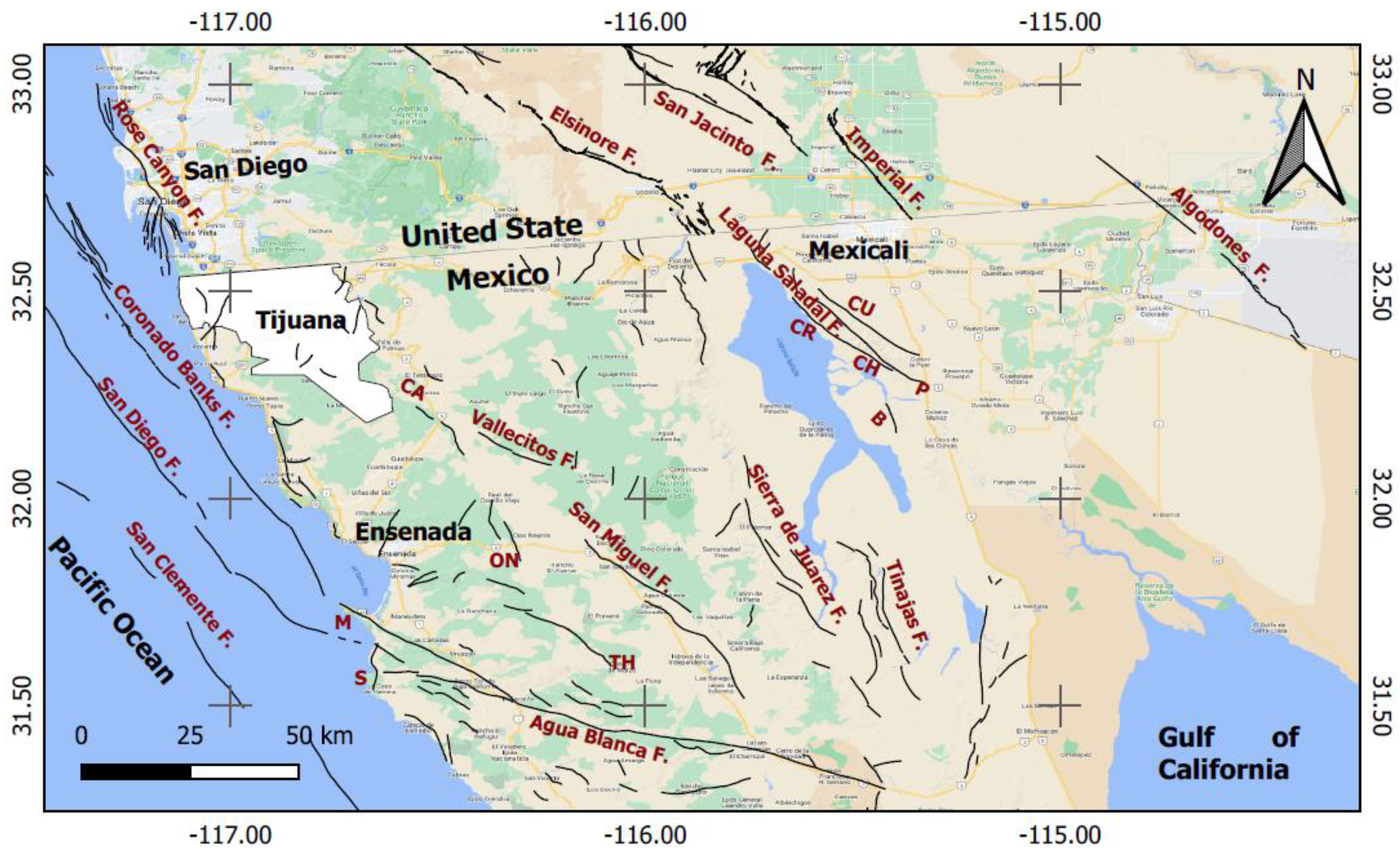
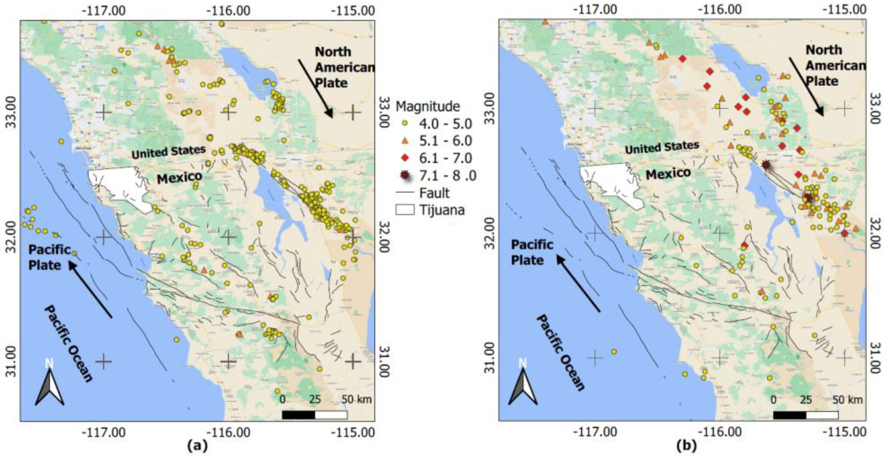
2. Seismicity of Baja California

The state of BC is located in a tectonically active zone. The region is subject to high seismic activitydue to its proximity to seismogenic zones associated with the interaction of the Pacific and North American plates [2,31]. BC is the eleventh most populous state in Mexico and is located in the northwest of the country. Baja California is divided into six municipalities.
The seismotectonic framework affecting the northwest of BC is composed of the following fault systems (Figure 1): Agua Blanca, the San Miguel–Vallecitos system, Ojos Negros, Tres Hermanos, Sierra Juárez, San Pedro Mártir, Calabazas, Maximinos, Pescaderos, and Bahía Soledad, the Rose Canyon–Newport system, Coronado Bank, San Diego, San Clemente, and Elsinore [31,32].
Regardingthe seismicity background in the region, a noteworthy earthquake occurred in the Mayor–Cucapah region in the Mexicali Valley on 4 April 2010, with a magnitude of 7.2. Additionally, in the central region of northern BC, the 1944 Guadalupe earthquake (M = 5.7) and the 1956 San Miguel earthquakes (M = 6.8, 6.4, and 6.3), located in the San Miguel–Vallecitos system, stand out, as does the 1934 earthquake (M = 5.9) associated with the San Clemente Fault on the continental edge. These seismic precedents indicate that anearthquake of significant magnitude should not be ruled out in the vicinity of the Pacific coastal strip in northern BC [31].
Figure 2 depicts the distribution of historical seismic events from 1800 to 2021 with magnitudes greater than 4.0 (Mw) in Southern California, Tijuana, and its surrounding areas in Mexico, as well as the activity of faults near the area of interest. Instrumental and historical events were extracted from the National Seismological Service [SSN] [33] and the United States Geological Survey [USGS] [34].

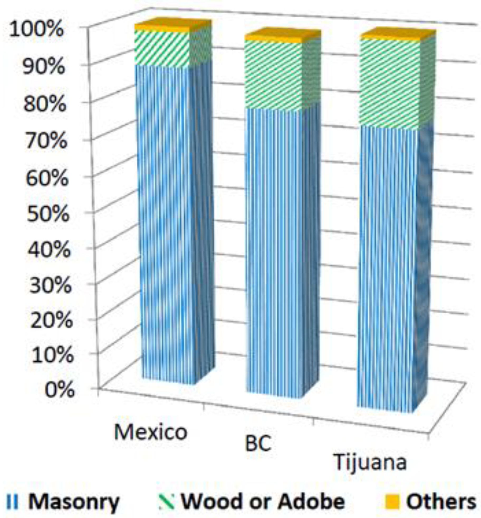
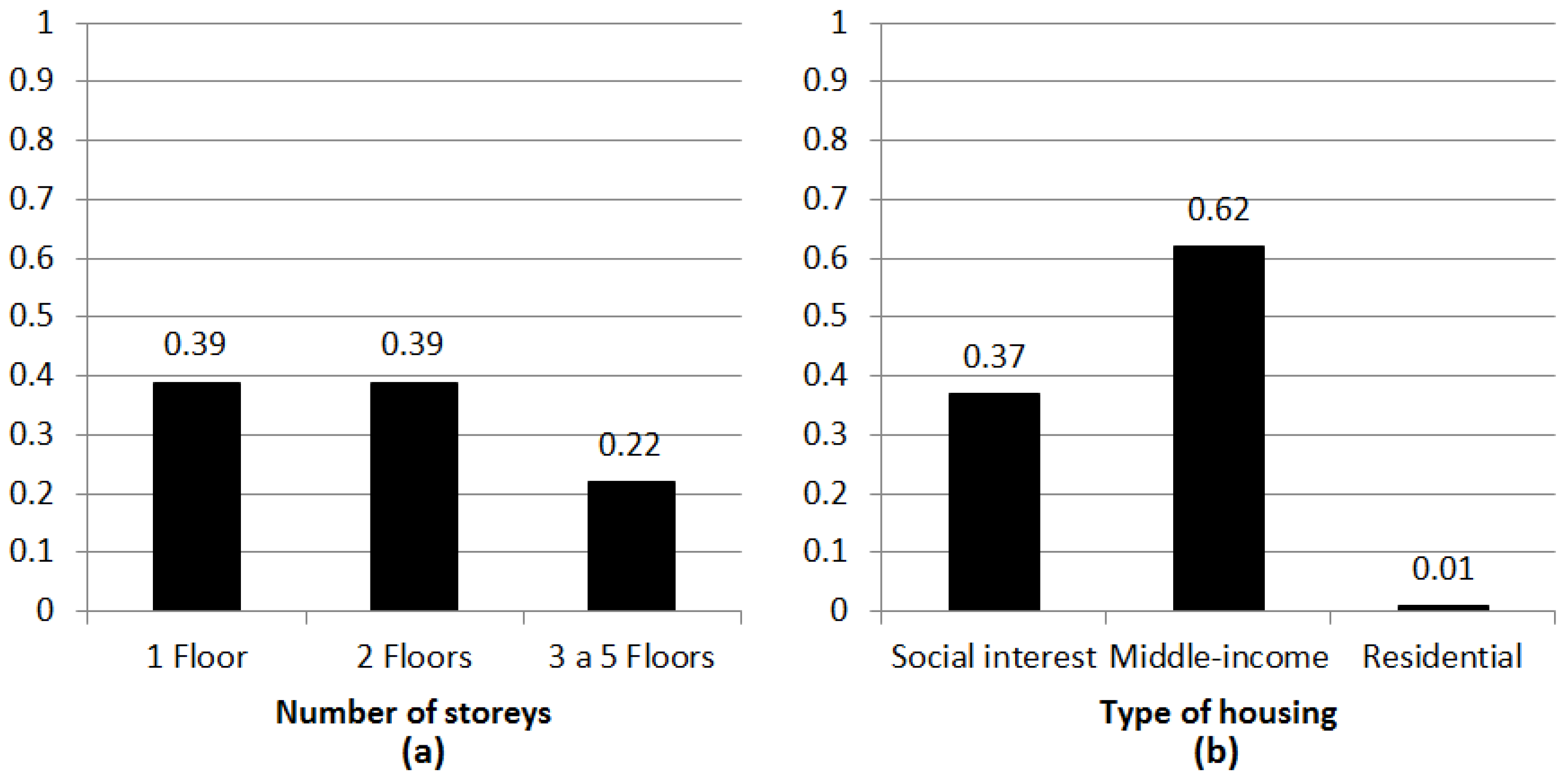
3. Identification of Common Housing Types in Tijuana

Baja California has a total of 1,148,913 housings, which accounts for 3.3% of the national total. Over 50% of the total housings in the city of Tijuana are concentratedwithin an area of 1074.1 km2 [35]. Based on the Intercensal Housing Survey conducted in the city of Tijuana in 2015, which aimed at collecting data on the city’s housing inventory, the following aspects are included: construction system, type of housing, number of levels, year of construction, and replacement value.
Regarding the construction system, at the national, state, and municipal levels, the most common construction materials, according to the distribution of the housing inventory, include masonry (brick, block, stone, and concrete), wood or adobe, and other materials (such as waste materials, cardboard, wattle and daub, asbestos or metal sheets, reeds, and unspecified materials). This is clearly evident in Figure 3, which highlights that over 75% of housings in the city of Tijuana are constructed using masonry materials [36]. Therefore, from an urban modeling perspective in the city, it is essential to pay special attention to homes that use masonry as a construction material.
In the census, type of housing is classified into five categories: house, apartment in a building, dwelling in a tenement, other types of dwellings, and unspecified dwellings, with houses being the dominant category with over 88% representation [36]. To determine the number of floors, as this information was not available in the census, a virtual survey was conducted, which involved taking a representative sample of housings from a total of 573 block clusters in the city of Tijuana. This was achieved using images available on the Google Street View application and the digital map of Mexico (http://gaia.inegi.org.mx/) (accessed on 15 February 2022). Each housing was classified into one of the following categories based on the number of floors: 1 floor, 2 floors, and 3 to 5 floors. Furthermore, housings were categorized into three types: social interest, middle-income, and residential (Figure 4). This last distinction is of paramount importance in a model, as it contributes to making accurate predictions of economic losses.
The year of construction was based on data provided by censuses conducted by the INEGI, covering a period from 1950 to 2020, as shown in Figure 5. This information is of great importance when assessing the vulnerability of existing buildings, as the year of construction can be used to determine the structural design code that was in effect at the time of construction. However, it is relevant to note that in the Tijuana region, many houses have been informally constructed, without adhering to the corresponding design codes.
The cost of housing is not reflected in the censuses conducted every ten years, so it was defined based on the construction area taken from virtual surveys. Regardless of the structural system, the following replacement costs were considered: for social interest houses, MXN 6413.03 (USD 320) per square meter;for medium-level houses, MXN 8680.40 (USD 434) per square meter;and for residential houses, MXN 13,478.89 (USD 673) per square meter. These values were defined based on the expert judgment of the College of Appraisers of Baja California A.C. in 2018.
The previous exposure model provides guidelines for categorizing masonry houses in the city of Tijuana. These categorizations have been subdivided considering their expected level of ductility, the number of floors, and the respective seismic design levels.
Table 1 presents a summary of the classification of masonry houses from 1 to 5 floors in the city of Tijuana. In this classification, vertical walls constitute the lateral force resistance system and can be either confined or reinforced masonry, designed for both ductile and non-ductile conditions, covering different seismic design levels in each taxonomy.
For each construction taxonomic rank, the seismic design level is defined and assigned. The following categories are considered [37]: a high level ofseismic design, H: the structure complies with all seismic requirements of national and international standards regarding load-bearing capacity and horizontal deformation capacity or ductility in high-seismic-hazard areas; a moderate level ofseismic design, M: the seismic-resistant specifications of the structure are associated with a medium level of compliance; and a low level of seismic design, L: the structure generally does not meet the minimum requirements for seismic-resistant design.

4. Vulnerability Modeller’sToolKit (VMTK)

The VMTK is a publicly accessible open-source toolkit available through a GitHub repository (https://github.com/GEMScienceTools/VMTK-Vulnerability-Modellers-ToolKit) (accesses on 14 March 2022). It was developed using the Python programming language with theaim to facilitate integration with other software that also utilizes this language, such as OpenQuake and OpenSees, for instance. The toolkit includes a graphical user interface (GUI) with graphic capabilities. The VMTK’s unique feature lies in its ability to integrate all stages of seismic vulnerability assessment within a single environment [24].
It is divided into six modules (a more detailed explanation of each module is available in Martins et al. 2021): (i) selection of ground motion records, (ii) definition of structural capacity, (iii) nonlinear dynamic analysis in single-degree-of-freedom (SDOF) oscillators to estimate the building’s response to seismic loads, (iv) conversion of dynamic analysis results into fragility functions, (v) derivation of vulnerability functions, and (vi) validation of results through the calculation of annual average losses and other common risk metrics.

4.1. Demand Module

This module is designed to assist the vulnerability modeler in the selection of appropriate ground motion records. In the current version of the VMTK, three options are presented for the selection and adjustment of these records.
The first alternative is to use all records provided by the user. The second option involves using a list of intensity levels, and the graphical user interface (GUI) includes a predefined list (PGA, SA (0.2 s), SA (0.3 s), SA (0.5 s), SA (0.6 s), SA (1.0 s), or SA (2.0 s)). The third option is based on the Conditional Spectrum Method (CSM).
It is essential to underline that the user must choose a set of ground motion records that meet the requirements of the vulnerability analysis. Regarding the list of intensities, the modeler can choose to select from the predefined list, but also has the flexibility to add custom intensities as needed. As for the CSM, this method involves conducting seismic risk disaggregation to understand the distribution of magnitude, distance, and epsilon at a specific location.

4.2. Capacity Module

In the VMTK, the capacity of structures is defined using bilinear, trilinear, or quadrilinear backbones. The capacity module processes capacity curves in the format of Acceleration Displacement Response Spectra (ADRS). The coordinates of the capacity curves can be input using the graphical user interface (GUI).

4.3. Structural Response Module

To calculate the nonlinear response of single-degree-of-freedom (SDOF) oscillators, the VMTK has been integrated with the open-source finite element modeling software OpenSees [38] through its Python implementation. Nonlinear behavior is introduced into numerical models through the uniaxial Pinching4 material and the capacity curves previously input by the user.

4.4. Fragility Module

The fourth module of the VMTK is dedicated to deriving fragility functions. After defining the relationship between structural response and ground shaking intensity, fragility functions are derived using the cloud analysis approach proposed by Jalayer et al. [39].
At this point, it is essential to have a damage model consisting of four damage states (DS): slight damage (DS1), moderate damage (DS2), extensive damage (DS3), and complete damage (DS4). Damage thresholds are defined using the yield (Sdy) and ultimate (Sdu) displacements from the capacity curves.

4.5. Vulnerability Module

For deriving vulnerability functions, two methodologies are implemented in the VMTK. In the first approach, the probability distribution of the loss rate is calculated using the resulting fragility model and a damage-to-loss model (i.e., the relationship between each damage state and the corresponding loss ratio).
The second methodology included in the tool follows the procedure described in Silva (2019) [40], in which loss rates (LR|IM) are directly calculated from the results of nonlinear dynamic analyses using a relationship between the engineering demand parameter and the expected loss rate.

4.6. Comparison and Results Verification Module

The last two modules of the VMTK provide the opportunity to compare the results with other available models, estimate risk metrics that can be compared with results from other models, or assess relative risk among different building categories. The GUI includes a comprehensive set of fragility and vulnerability functions extracted from the GEM vulnerability database. Users can also compare the results of fragility or vulnerability matrices from other models. Furthermore, the toolkit allows for the calculation of common risk metrics using the resulting fragility or vulnerability functions and seismic hazard curves defined in the OpenQuake format.

5. Case Study

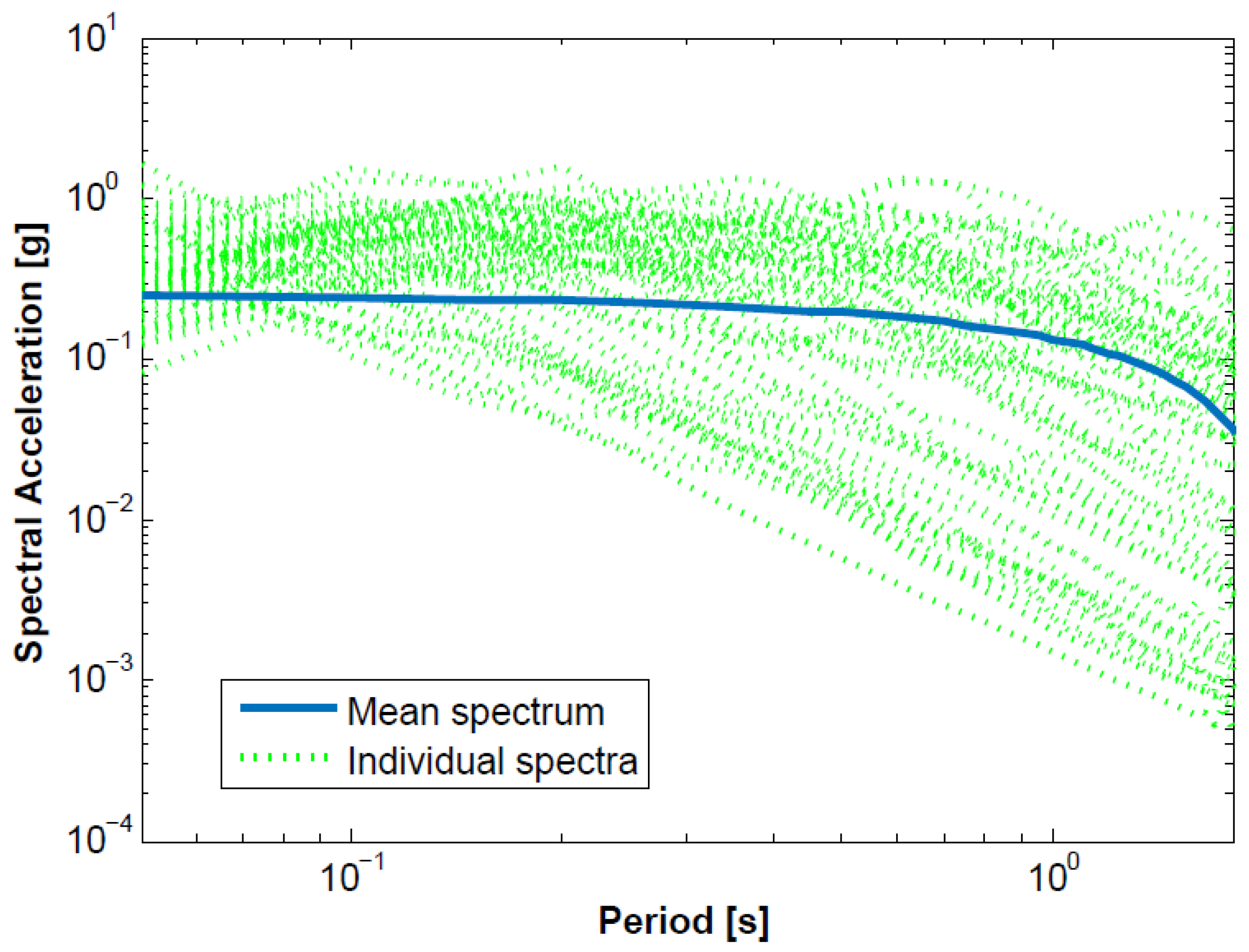
5.1. Selection of Ground Motion Records

The probabilistic method defined by Cornell was used to calculate seismic hazard in the city of Tijuana [41]. Data processing was carried out using the EPPS14 program [31,42], which wasdeveloped in the Matlab language. The linear sources used in the EPPS14 program represent faults or fault segments in the region based on the segmentation proposed by Anderson et al. and Munguía [42,43]. These correspond to active faults with the potential to generate significant magnitude earthquakes that could affect civil structures. The points of interest where this method was applied were within the city of Tijuana, specifically at the locations of stations that make up the Tijuana Strong-Motion Network. The stations include PR = Presa Abelardo L. Rodríguez, TUN = Tanque Aguaje de la Tuna, COL = Tanque Cerro Colorado, PLA = Planta de Tratamiento Playas, PCI = TerrenoProtección Civil, and CCC = Centro Control, Comando y Computo de la Policía (Table 2).
Using EPPS14, seismic hazard disaggregation was determined for each site of interest. A summary of the results for each of the sites is presented in Table 3. The results obtained, considering the linear sources and the calculation of the uniform hazard spectrum at each specific site, were used for the selection of records based on tectonic setting, magnitude, and distance.
The seismic demand requested by the VMTK was integrated using the accelerometer records for our study area that met the aforementioned characteristics (Figure 6). The following ground motion databases were selected for the records: the Center for Engineering Strong Motion (CESMD) [45] (Table 4) and the Northwestern Mexico Accelerograph Network (RANM) [46] (Table 5).

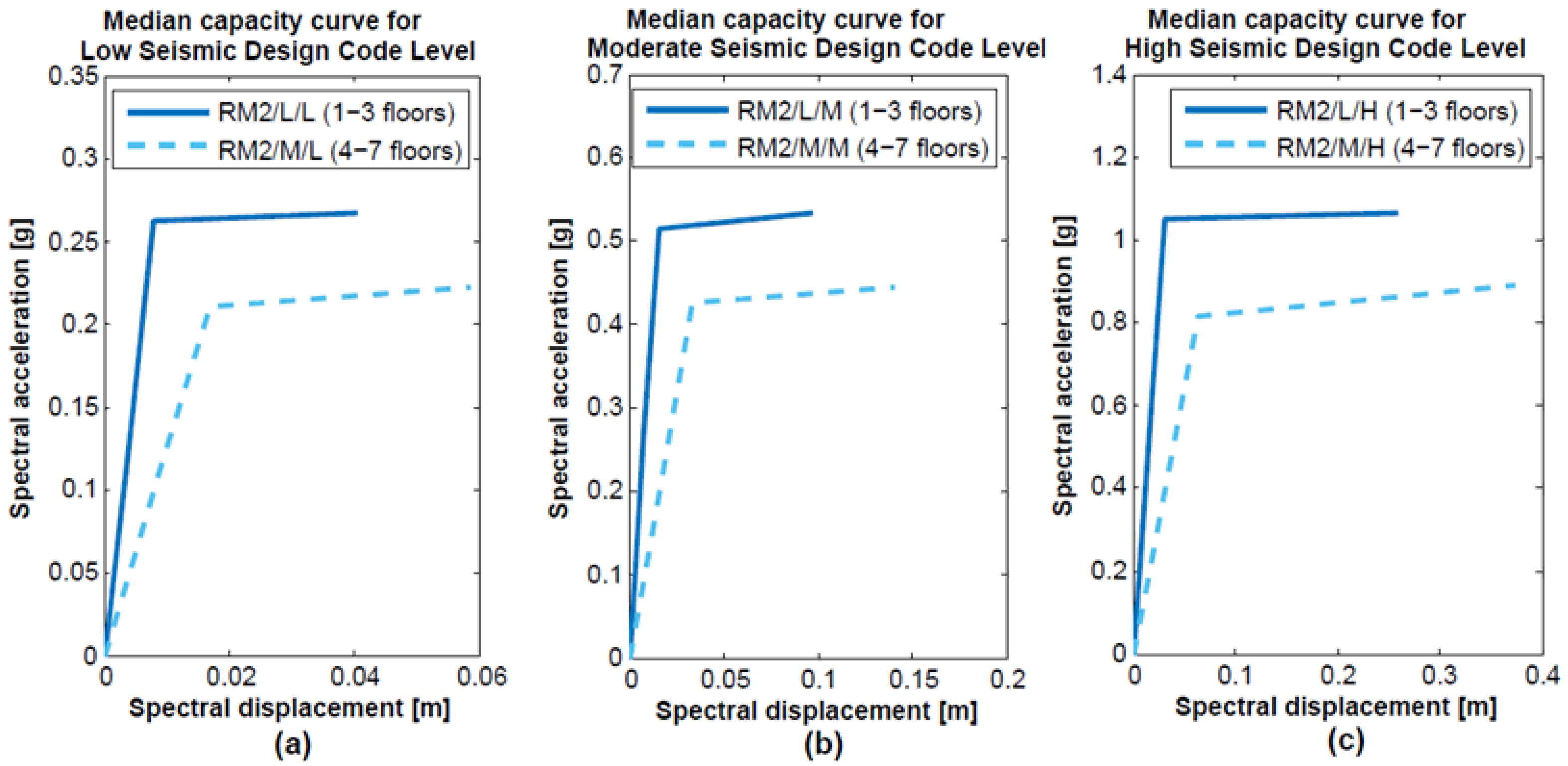
5.2. Capacity Curves

ConsideringTijuana’s status as a border city with the United States, typologies with capacity curves and similar characteristics developed in the HAZUS manual [21] were sought, with the closest match being typologies RM2/L and RM2/M, corresponding to masonry shear wall buildings with low (1–3 stories) and medium (4–7 stories) concrete diaphragms, respectively (Table 6). Each HAZUS capacity curve for buildings is a graph that shows the lateral resistance of a building as a function of a characteristic lateral displacement. It is derived from a graph of the equivalent static base shear versus the building’s displacement. To make it easier to compare it to earthquake force (i.e., by overlaying the capacity curve with a response spectrum), we transformed the axis representing force into one that shows spectral acceleration and the axis representing displacement into one indicating spectral displacement.
The capacity curves defined by HAZUS are given by the yield point (Dy, Ay) and the maximum capacity point (Du, Au). The yield capacity represents the true lateral resistance of the building, considering redundancies in design, conservatism in code requirements, and actual material strength. The maximum capacity represents the maximum strength of the building when the overall structural system has reached a fully plastic state. HAZUS provides only the values of these two points, so the curves were reconstructed using a fourth-degree polynomial while ensuring the following conditions are met: (1) the curve passes through the yield point (Dy, Ay); (2) the curve passes through the maximum capacity point (Du, Au); (3) the curve is linear from the origin to the yield point; (4) the curve retains the initial slope at the yield point; and (5) the curve is horizontal at the maximum capacity point.
The capacity curve was transformed into a bilinear capacity curve to obtain an idealized representation, following the ATC-40 procedure [47], where a yield point A with coordinates (dy, ay) and an assumed performance point B with coordinates (Du, Au) are defined, and the area designated as A1 is approximately equal to the area designated as A2 [48].
Figure 7 shows the idealized bilinear HAZUS capacity curves for buildings with reinforced masonry low-rise (RM2/L) and medium-rise (RM2/M)load-bearing walls, with low (L), moderate (M), and high (H) seismic design code levels.

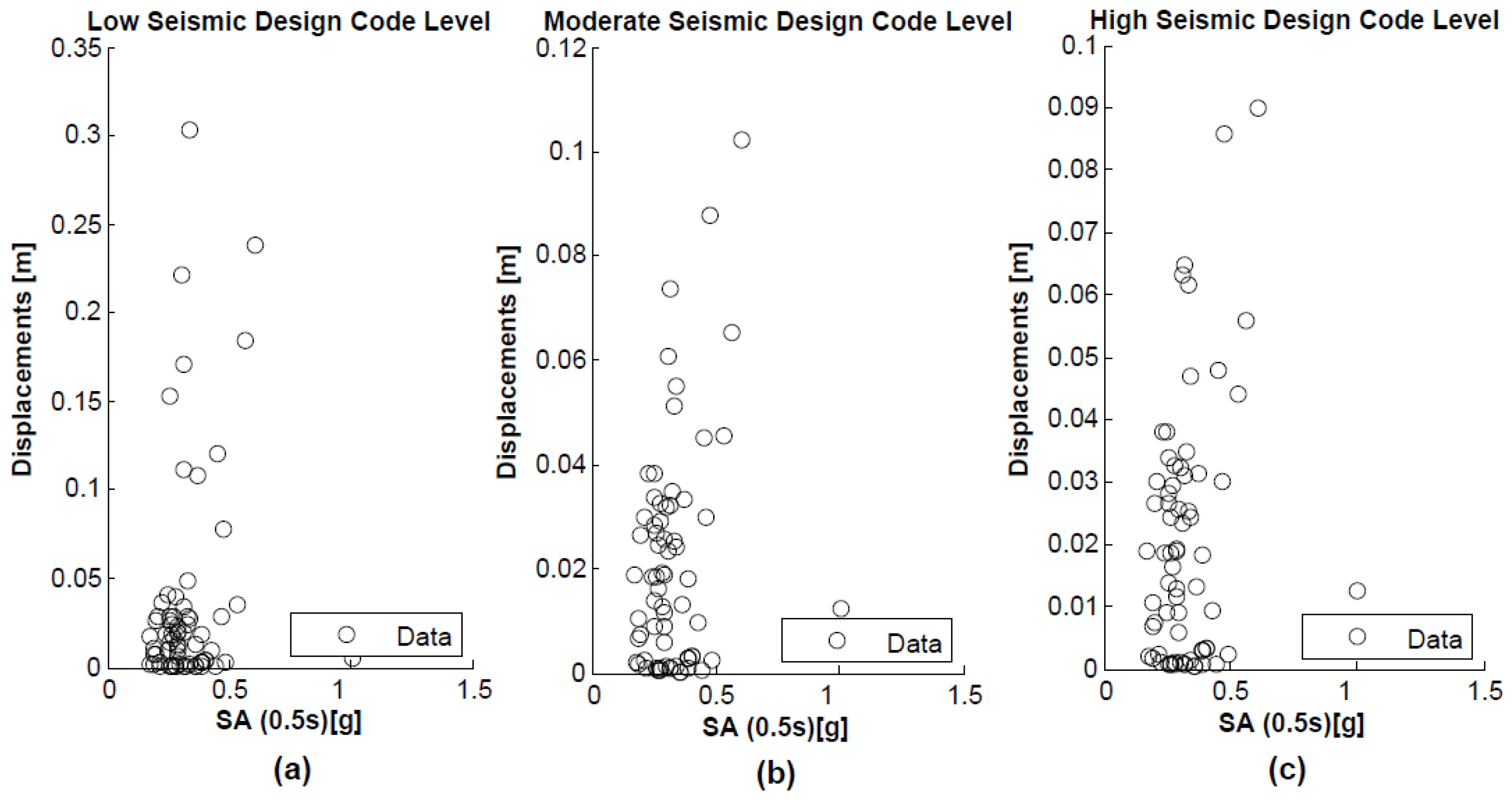
5.3. Structural Response

After conducting the structural analyses, thedistribution of engineering demand parameters (EDPs) against intensity measure (IM) levels wasgenerated with the VMTK, which wasthen used for the derivation of fragility functions. Two types of IM were defined as representative of the dynamic characteristics for building classes: peak ground acceleration (PGA) for housing (one to three floors) (Figure 8) and spectral acceleration (Sa) of 0.5 s for a housing with four to seven floors (Figure 9). The selection of 0.5 s was based on the elongated period to account for the effect of structural damage on the dynamic properties of the housing census [49].

5.4. Definition of Damage Criterion

Four potential damage states were considered, ranging from minor (DS1) to moderate (DS2), extensive (DS3), and complete (DS4). This study closely followedthe proposal ofLagomarsinoandGiovinazzi [11]. Minor damage occurs when 70% of the spectrum exceeds the displacement at the yield point (i.e., 0.70 Sdy); the threshold for moderate damage, which is higher than that for extensive damage, is defined as (0.75 Sdy + 0.25 Sdu). The threshold for extensive damage is defined as the average between the spectral yield point displacement and ultimate displacement (i.e., (Sdy + Sdu)/2), and it is considered complete when the ultimate displacement is exceeded (i.e., Sdu) [50].

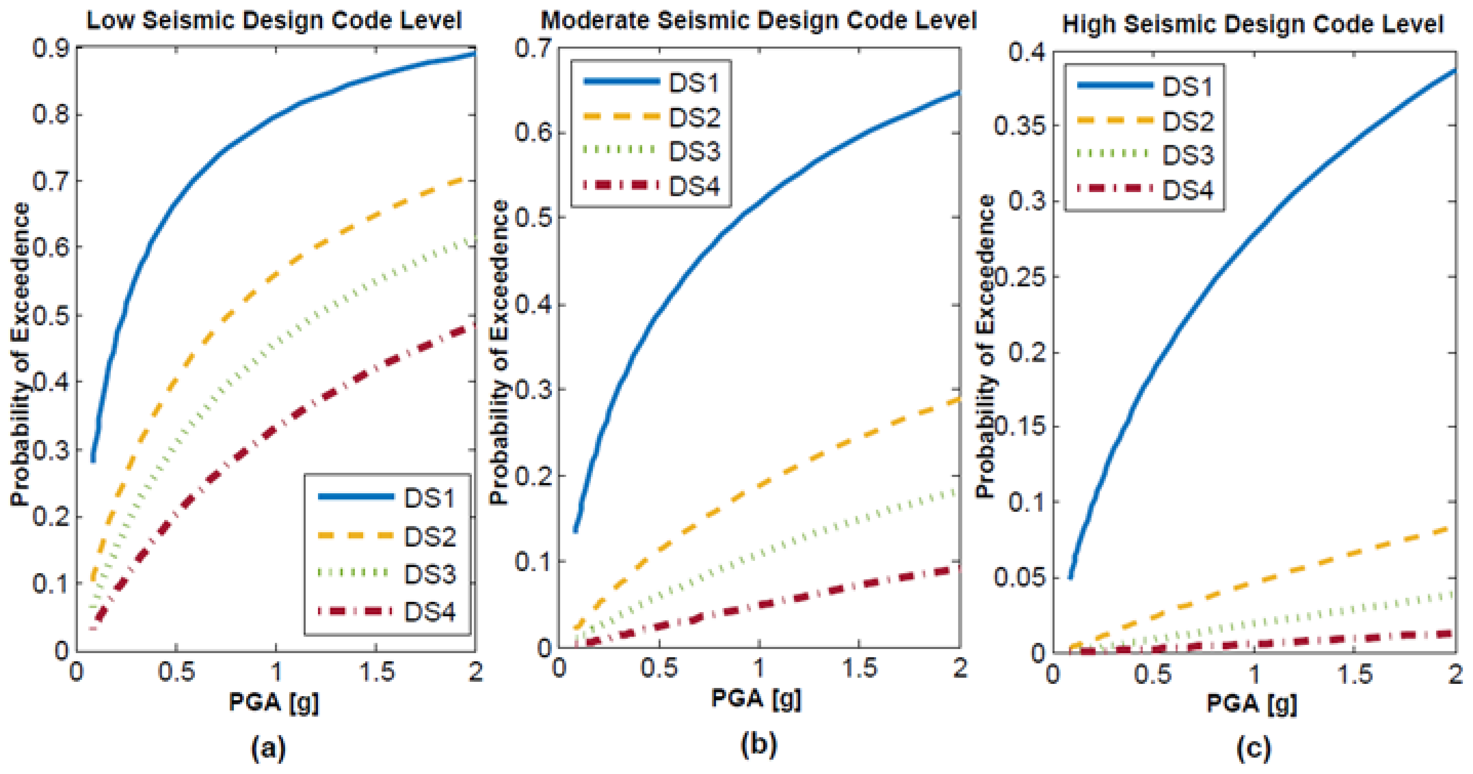
5.5. Derivation of Fragility Functions

The cloud analysis [39] requires defining a best-fit curve between an intensity measure (IM) and an engineering demand parameter (EDP) in the logarithmic space.
The regression algorithm was implemented in the toolkit, where excessively high displacements are treated differently through censored regression analysis [51]. This regression method is based on the fact that numerical analyses can achieve convergence for displacement levels that are incompatible with structural stability. This mainly occurs due to limitations in numerical modeling and can introduce biases into the best-fit curve. Censored regression analysis requires defining a threshold (i.e., maximum displacement or acceleration), beyond which data points are assumed to be affected by numerical errors. This threshold is defined by a censoring factor, which is defined as the ratio between the maximum allowable EDP and the threshold for the last considered damage state (e.g., complete damage). In this case, a censoring factor of 1.5 was used, meaning that EDPs 1.5 times above the threshold for the last damage state will be treated differently [23,24].
As explicit consideration of building-to-building variability was not accounted for (i.e., only one capacity curve was provided per building class), it waspossible to increase uncertainty to account for this source of variability. In the VMTK, this adjustment wasmade by adding to the dispersion of variability from record to record (σrec-to-rec) [24]. In other words, two records with the exact same IM can result in different structural responses due to the contribution of building-to-building variability (σbld-to-bld). For simplicity’s sake, we chose to directly increase the standard deviation around the best-fit curve by a factor of 0.30, as described in Equation (1) [23].
σ t o t a l = σ r e c t o r e c 2 + σ b l d t o b l d 2
The resulting fragility functions are defined using cumulative log-normal functions, as shown in Figure 10 and Figure 11 for the aforementioned structure classes.
The fragility functions derived from low- and medium-rise masonry houses werecompared for different seismic design levels. Table 7 provides a summary of the probability of reaching or exceeding various damage states for low-rise houses (RM2/L) at an expected value of 0.50 g of PGA and for medium-rise houses (RM2/M) at an expected value of 0.5 g of SA (T = 0.5 s). For example, it can be observed that the probability of damage decreasedfor low-rise houses (RM2/L) with moderate and high levels of seismic design, especially for damage states DS3 and DS4, and the probability of damage waszero for medium-rise houses (RM2/M) in damage state DS4 for moderate and high levels of seismic design.

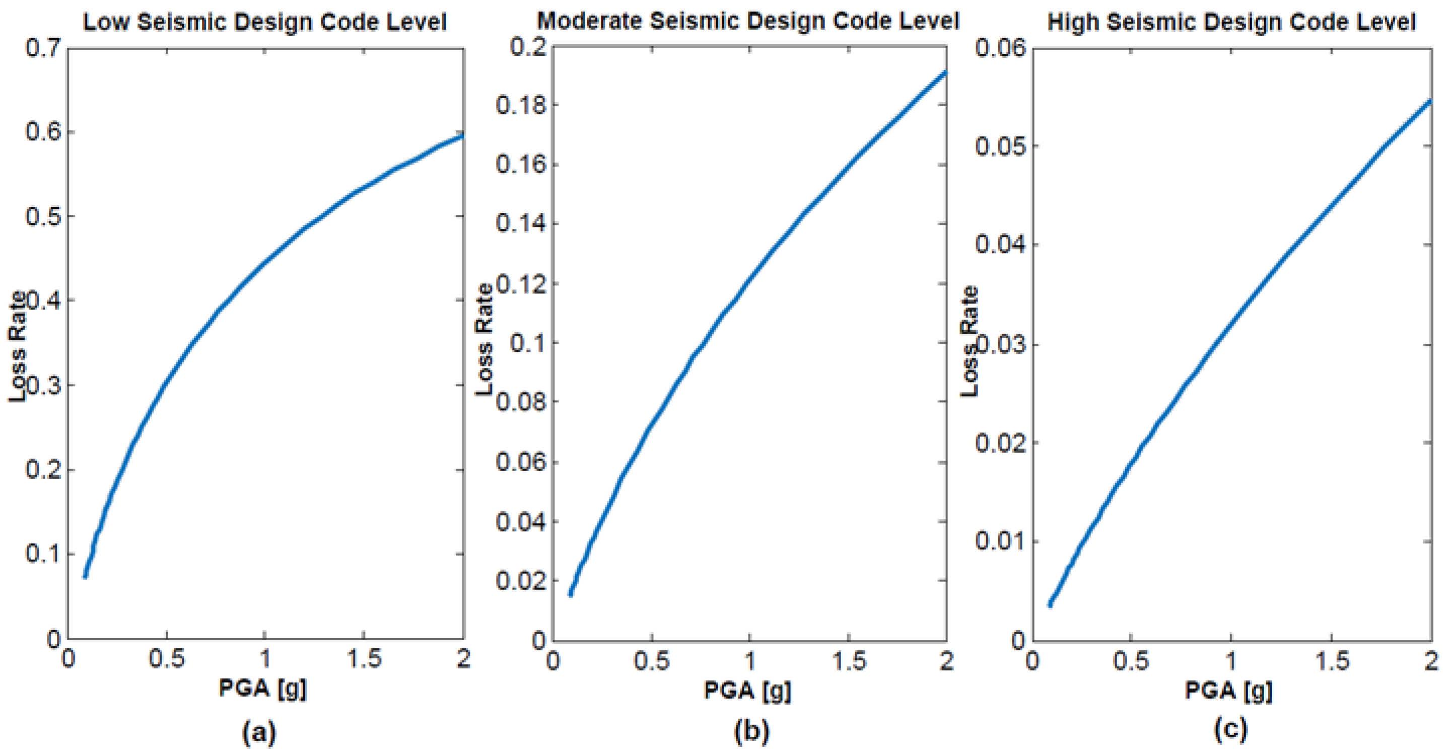
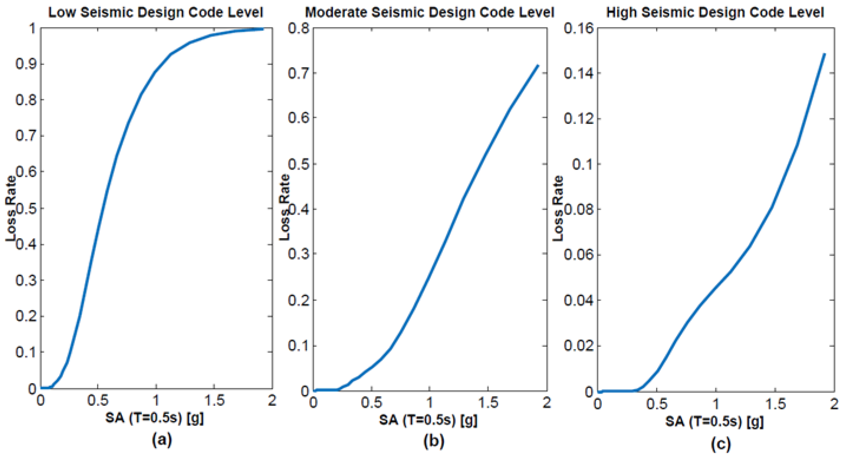
5.6. Vulnerability Functions

Fragility functions are often transformed into vulnerability functions that can be subsequently used in loss assessment [52]. The VMTK wasalso employed in deriving these curves by calculating the probability distribution of the loss rate using the resulting fragility model and a damage-to-loss relationship model (i.e., the relationship between each damage state and the corresponding loss rate).
The damage-to-loss model used is the one described in FEMA [53], where the expected loss rates for each damage state are as follows: slight damage (LR) = 0.05, moderate damage (LR) = 0.25, extensive damage (LR) = 0.60, and complete damage (LR) = 1.00.
The average loss rate of the vulnerability functions at each level of intensity measurement (LR|IM) is equal to the result of multiplying the probability of each damage state (P [DS = dsi|IM]) by the associated average loss rate (LRdsi), as described in Equation (2) [24].
L R | I M = i = 1 n D S P D S = d s i | I M × L R d s i
Following this procedure and utilizing the fragility functions and the damage-to-loss model presented earlier, the vulnerability functions were obtained, as depicted in Figure 12 and Figure 13.
Table 8 presents a summary of the probability of loss ratio in low-rise (RM2/L) and mid-rise (RM2/M) buildings for an expected value of 0.50 g of PGA and 0.50 g of SA (T = 0.5 s), respectively. For example, it can be observed that the loss ratio wasminimal for low-rise (RM2/L) and mid-rise (RM2/M) buildings with a moderate and high seismic design. For a low seismic design, both low-rise and mid-rise structures hada 30% and 44% probability of loss ratio, respectively.

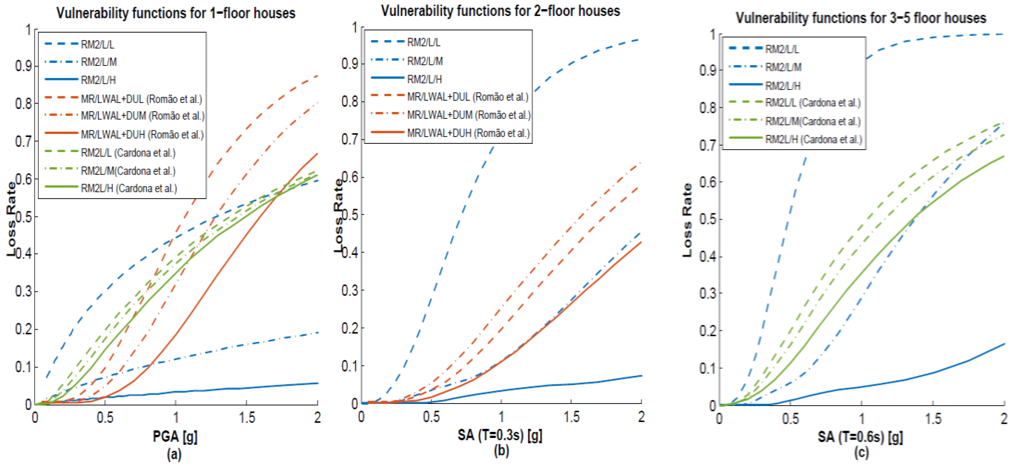
5.7. Comparison of Results

In the case of single-floor houses constructed with reinforced masonry, the damage assessment is closely related to the maximum ground acceleration (PGA). On the other hand, for two-floor and three-tofive-floor houses, the damage assessment is directly related to spectral acceleration, specifically SA (T = 0.3 s) and SA (T = 0.6 s), respectively. This allows us to more accurately assess the vulnerability of different types of houses to seismic events. Furthermore, to compare our results with other studies, we calculated vulnerability functions using the previously mentioned procedures for two spectral acceleration values: SA (T = 0.3 s) and SA (T = 0.6 s).
Figure 14 presents vulnerability functions specifically designed for reinforced masonry structures, developed by severalauthors. Among these, Romão et al. created functions for European houses, classifying them into three ductility levels: low (DUL), moderate (DUM), and high (DUH) [54]. Likewise, Cardona contributed functions with global applicability, suitable for various seismic threats, following the HAZUS methodology [37]. The functions presented in this article, like those of Cardona et al., are divided into three categories corresponding to low (L), moderate (M), and high (H) seismic levels.
Table 9 presents a summary reflecting the probabilities of loss rates in different types of houses, including one-floor, two-floor, and three-tofive-floor reinforced masonry houses. These probabilities werecalculated considering a spectral acceleration of 0.5 g and compared with historical accelerations recorded in the study area, which can vary in the range of 0.20 to 0.50 g [29].
When analyzing the loss rates in vulnerability functions proposed by various authors for one-floor houses, considering a low seismic design level, significant differences can be observed. In particular, Romão et al. present a loss rate of 9.7%, while Cardona et al. and the results of this article show significantly higher figures, at19.7% and 30%, respectively.
For these same one-floor houses, when considering moderate and high seismic design levels, Romão et al. reported loss rates of 4.7% and 1.8%, respectively. These values show similarity with the results obtained in this article, at 7% and 1%, respectively.
The vulnerability functions proposed in this article were compared with the Romão et al. functions, considering two-floor houses and their three seismic design levels: low, moderate, and high. In the case of houses with a low seismic design level, this article reveals a 30% higher loss rate compared to the loss rate presented by Romão et al., which is 5.3%. However, a similarity wasobserved in the loss rate in cases of moderate and high seismic design.
A comparison was made between the vulnerability functions presented in this study and those developed by Cardona et al. for three-to-five-floor houses in three seismic design levels: low, moderate, and high. In all cases, it is evident that the loss rate is lower than what is presented in this work.

6. Conclusions

Some researchers have developed fragility and vulnerability functions for various building classes in different parts of the world, achieving promising results through open-access programs [5,23,24,49,50]. In the preceding sections, the probability of damage and loss was determined using a set of ground motion records characteristic of the region [45,46]. The analysis was conducted on masonry houses in the city of Tijuana, BC, which, according to data from [35], represents over 432,000 housings. The open-source platform VMTK was employed, offering a viable option for determining fragility and vulnerability functions for various types of structures in the region and around the world. Before using it, it is essential to review its limitations and necessary features to ensure it can be easily adapted.
The fragility models were developed following the cloud analysis method proposed by [39] and nonlinear time history analysis in equivalent SDOF oscillators. The derived fragility functions for low- and medium-rise masonry houses were compared for different seismic design levels. It was observed that the probability of damage decreases in low-rise houses for all damage states with moderate and high seismic design levels. Additionally, there is a 20% probability of reaching damage state DS4 for low-rise houses with a low seismic design level, considering an expected value of 0.50 g of PGA. For medium-rise houses, there is no damage in DS2, DS3, and DS4 with a high seismic design level. Furthermore, there is a 16% probability of reaching damage state DS4 for medium-rise houses with a low level of seismic design, considering an expected value of 0.50 g of SA (T = 0.5 s).
In BC, over 50% of housings exhibit structural damage [35], stemming from a substantial portion of informal construction carried out over the years with low or nonexistent design standards, resulting in increased vulnerability of housings in the event of an earthquake. When deriving vulnerability functions, it was determined that for a low seismic design level, structures with 1–3 stories and 4–7 stories in height have a higher probability of loss indices, at 30% and 44%, respectively, for an expected value of 0.50 g of PGA and SA (T = 0.5 s).
When comparing vulnerability functions for single-floor and two-floor houses with a low seismic design level, it is noteworthy that the results of this article reveal a significantly higher loss index, reaching 30%, surpassing that found by other authors. Similarly, for three- to five-floor houses, the loss index also significantly increases to 52%, positioning it above values obtained by other researchers.
For single-floor houses with a moderate and high seismic design level, it can beobserved that the loss indices obtained in this study, which are 7% and 1.8%, respectively, are lower than those presented by Cardona et al. [37]. Conversely, these results show similarities with the values obtained by Romão et al. [54].
In the case of two-floor houses with a moderate seismic design level, a notable similarity can beobserved between the results presented by Romão et al. [54] and those of this study. On the other hand, for three- to five-floor houses with a moderate and high seismic design level, the values obtained in this study, which are 6% and 1%, respectively, are lower than those presented by Cardona et al. [37].
A comparison has been made between the vulnerability functions obtained in this article and those developed by other authors in different regions around the world, revealing significant discrepancies. These disparities could introduce greater uncertainty in damage and loss estimation in risk scenarios.
In the specific case of the city of Tijuana, which is located in a high-seismic-activity zone, there areno available data regarding the damage caused by earthquakes prior to the generation of these vulnerability functions. Furthermore, there is no regulatory section addressing the specific use of vulnerability functions for masonry houses. This has led other authors, such as Gonzales, Rodríguez, and Romero [2,29,30], to utilize vulnerability functions from other parts of the world for their risk assessments.
This work introduces a procedure grounded in open-access methodologies, providing the opportunity for other users, especially those with limited access to data and information, to develop their own vulnerability functions tailored to their study area and various types of structures. These functions can be employed to estimate damage and losses in risk situations, playing a crucial role in reducing uncertainty in risk analysis calculations.

Author Contributions

Conceptualization and methodology, F.-D.D. and M.G.-D.; software, F.-D.D. and D.-L.F.; validation, formal analysis, investigation, resources, data curation and writing—original draft preparation, F.-D.D.; writing—review and editing, F.-D.D., M.G.-D., D.-L.F., A.L.-L., U.M.-H. and M.V.-C.; supervision, M.G.-D. All authors have read and agreed to the published version of the manuscript.

Funding

Francisco Diaz is a doctoral student in the ProgramaMaestría y DoctoradoenCiencias e Ingeniería, Universidad Autónoma de Baja California (UABC) and received a fellowship, 229426, from CONACyT.

Institutional Review Board Statement

Not applicable.

Informed Consent Statement

Not applicable.

Data Availability Statement

The data presented in this study are available on request from the corresponding author.

Conflicts of Interest

The authors declare no conflict of interest.

References

  1. Imjai, T.; Setkit, M.; Garcia, R.; Sukontasukkul, P.; Limkatanyu, S. Seismic strengthening of low strength concrete columns using high ductile metal strap confinement: A case study of kindergarten school in Northern Thailand. Walailak J. Sci. Technol. 2020, 17, 1335–1347. [Google Scholar] [CrossRef]
  2. Rodríguez-Valenzuela, L.M.; Mungaray-Moctezuma, A.; González-Durán, M.; Mena-Hernández, U. Structural damage to housing and effects on users due to seismic risk: A case study. Proc. Inst. Civ. Eng.-Munic. Eng. 2020, 174, 120–135. [Google Scholar] [CrossRef]
  3. Ruggieri, S.; Liguori, F.S.; Leggieri, V.; Bilotta, A.; Madeo, A.; Casolo, S.; Uva, G. An archetype-based automated procedure to derive global-local seismic fragility of masonry building aggregates: META-FORMA-XL. Int. J. Disaster RiskReduct. 2023, 95, 103903. [Google Scholar] [CrossRef]
  4. Cardinali, V.; Tanganelli, M.; Bento, R. A hybrid approach for the seismic vulnerability assessment of the modern residential masonry buildings. Int. J. Disaster Risk Reduct. 2022, 79, 103193. [Google Scholar] [CrossRef]
  5. Martins, L.; Silva, V. A global database of vulnerability models for seismic risk assessment. In Proceedings of the 16th European Conference on Earthquake Engineering, Thessaloniki, Greece, 18–21 June 2018. [Google Scholar]
  6. Silva, V.; Crowley, H.; Varum, H.; Pinho, R.; Sousa, R. Evaluation of analytical methodologies used to derive vulnerability functions. Earthq. Eng. Struct. Dyn. 2014, 43, 181–204. [Google Scholar] [CrossRef]
  7. Yamin, L.E.; Hurtado, A.; Rincon, R.; Dorado, J.F.; Reyes, J.C. Probabilistic seismic vulnerability assessment of buildings in terms of economic losses. Eng. Struct. 2017, 138, 308–323. [Google Scholar] [CrossRef]
  8. Kassem, M.; Mohamed Nazri, F.; NoroozinejadFarsangi, E. The seismic vulnerability assessment methodologies: A state-of-the-art review. Ain Shams Eng. J. 2020, 11, 849–864. [Google Scholar] [CrossRef]
  9. Whitman, R.; Reed, J.; Hong, S.-T. Earthquake Damage Probability Matrices. In Proceedings of the Fifth World Conference on Earthquake Engineering, Rome, Italy, 25–29 June 1974; pp. 2531–2540. [Google Scholar]
  10. Benedetti, D.; Benzoni, G.; Parisi, M.A. Seismic vulnerability and risk evaluation for old urban nuclei. Earthq. Eng. Struct. Dyn. 1988, 16, 183–201. [Google Scholar] [CrossRef]
  11. Lagomarsino, S.; Giovinazzi, S. Macroseismic and mechanical models for the vulnerability and damage assessment of current buildings. Bull. Earthq. Eng. 2006, 4, 415–443. [Google Scholar] [CrossRef]
  12. Baggio, C.; Bernardini, A.; Colozza, R.; Corazza, L.; Della Bella, M.; Di Pasquale, G.; Dolce, M.; Goretti, A.; Martinelli, A.; Orsini, G.; et al. Manuale per la Compilazionedellascheda di Primo Livello di Rilevamentodanno, Pronto Intervento e Agibilità per Edificiordinarinell’emergenzapost-sismica (AEDES), Italy. 2014. Available online: https://www.protezionecivile.gov.it/it/pubblicazione/manuale-la-compilazione-della-scheda-di-primo-livello-di-rilevamento-di-danno-pronto-intervento-e-agibilita-edifici-ordinari-nellemergenza-post/ (accessed on 5 September 2023).
  13. FEMA P-155; FEMA-155: Rapid Visual Screening of Buildings for Potential Seismic Hazards: Supporting Documentation. Federal Emergency Management Agency: Washington, DC, USA, 2015.
  14. Rosti, A.; Rota, M.; Penna, A. Empirical fragility curves for Italian URM buildings. Bull. Earthq. Eng. 2021, 19, 3057–3076. [Google Scholar] [CrossRef]
  15. D’Ayala, D. Assessing the seismic vulnerability of masonry buildings. In Handbook of Seismic Risk Analysis and Management of Civil Infrastructure Systems; Elsevier: Amsterdam, The Netherlands, 2013. [Google Scholar] [CrossRef]
  16. D’Ayala, D.; Speranza, E. Definition of Collapse Mechanisms and Seismic Vulnerability of Historic Masonry Buildings. Earthq. Spectra. 2003, 19, 479–509. [Google Scholar] [CrossRef]
  17. D’Ayala, D. Force and displacement based vulnerability assessment for traditional buildings. Bull. Earthq. Eng. 2005, 3, 235–265. [Google Scholar] [CrossRef]
  18. Borzi, B.; Crowley, H.; Pinho, R. Simplified pushover-based earthquake loss assessment (SP-BELA) method for masonry buildings. Int. J. Archit. Herit. 2008, 2, 353–376. [Google Scholar] [CrossRef]
  19. Kappos, A.; Panagopoulos, G.; Penelis, G. Development of a seismic damage and loss scenario for contemporary and historical buildings in Thessaloniki, Greece. Soil Dyn. Earthq. Eng. 2008, 28, 836–850. [Google Scholar] [CrossRef]
  20. Molina, S.; Lang, D.; Lindholm, C. SELENA—An open-source tool for seismic risk and loss assessment using a logic tree computation procedure. Comput. Geosci. 2010, 36, 257–269. [Google Scholar] [CrossRef]
  21. FEMA. Hazus–MH 2.1: Technical Manual; Federal Emergency Management Agency: Washington, DC, USA, 2012. [Google Scholar]
  22. Silva, V.; Casotto, C.; Rao, A.; Villar, M.; Crowley, H.; Vamvatsikos, D. OpenQuake Risk Modeller’s Toolkit—User Guide. Glob. Earthq. Model (GEM) Tech. Rep. 2015, 9, 97. [Google Scholar]
  23. Martins, L.; Silva, V. Development of a fragility and vulnerability model for global seismic risk analyses. Bull. Earthq. Eng. 2020, 19, 6719–6745. [Google Scholar] [CrossRef]
  24. Martins, L.; Silva, V.; Crowley, H.; Cavalieri, F. Vulnerability modellers toolkit, an open-source platform for vulnerability analysis. Bull. Earthq. Eng. 2021, 19, 5691–5709. [Google Scholar] [CrossRef]
  25. NTCBC. Normas Técnicas Complementarias de la Ley de Edificaciones del Estado de Baja California, de Seguridad Estructural en Materia de “Diseño y Construccion de Mamposteria”; NTCBC: Mexico City, Mexico, 2017. [Google Scholar]
  26. Rosquillas, A.; Mendoza, L. Proyecto RADIUS Case Tijuana (Risk Assessment Tools for Diagnosis of Urban Areas against Seismic Disasters), 2nd ed.; CICESE and XVI District Council of Tijuana: Tijuana, Mexico, 2000; pp. 27–28. [Google Scholar]
  27. Garatachia, J.C.; Baró Suárez, J.E.; Huerta López, C.I. Chapter 1. Book: Aproximación a la vulnerabilidad estructural y socioeconómica en el marco de un estudio de riesgo sísmico en la zona urbana de Tijuana, Baja California. In Vulnerabilidad Territorial ante la Expansión Urbana; Universidad of Mexico: Mexico City, Mexico, 2016. [Google Scholar]
  28. Cardona, O.; Ordaz, M.; Reinoso, E. CAPRA–comprehensive approach to probabilistic risk assessment: International initiative for risk management effectiveness. In Proceedings of the 15th World Conference on Earthquake Engineering, Lisbon, Portugal, 24–28 September 2012; Volume 1, p. 10. Available online: http://www.iitk.ac.in/nicee/wcee/article/WCEE2012_0726.pdf (accessed on 21 August 2023).
  29. González, M. Impacto Socioeconómico del Daño Estructural por Sismo en Viviendas de 1 y 2 Niveles en las Ciudades de Baja California, México. Ph.D. Thesis, Universidad Autónoma de Baja California, Mexicali, Mexico, 2016. [Google Scholar]
  30. Romero, P. Escenario de Riesgo Sísmico en la Ciudad de Tijuana, Baja California, México. Master’s Thesis, Universidad Autónoma de Baja California, Mexicali, Mexico, 2020. [Google Scholar]
  31. Arce, R. Estimación de Peligro Sísmico en el Norte de BC, con Aplicación en el Cálculo de la Respuesta Dinámica de dos Edificios. Master’s Thesis, Centro de Investigación Científica y de Educación Superior de Ensenada, Ensenada, Mexico, 2016. Available online: http://cicese.repositorioinstitucional.mx/jspui/handle/1007/956 (accessed on 15 February 2022).
  32. Soares, J. Aplicación de la microzonación sísmica a la seguridad de estructuras críticas en la ciudad de Ensenada. Master’s Thesis, Centro de Investigación Científica y de Educación Superior de Ensenada, Ensenada, Mexico, 2003. [Google Scholar]
  33. Servicio Sismológico Nacional (SSN). EarthquakeCatalog. Available online: http://www.ssn.unam.mx/ (accessed on 1 March 2022).
  34. United States Geological Survey (USGS). Earthquake Catalog. Available online: https://www.usgs.gov/programs/earthquake-hazards/earthquakes (accessed on 1 March 2022).
  35. INEGI. Panorama Sociodemográfico de Baja California, Mexico, 2021, INEGI (Instituto Nacional de Estadística y Geografía). Available online: https://www.inegi.org.mx/contenidos/productos/prod_serv/contenidos/espanol/bvinegi/productos/nueva_estruc/702825197735.pdf (accessed on 15 February 2022).
  36. INEGI. Anuario Estadístico y Geográfico de Baja California, Mexico, 2017, INEGI (Instituto Nacional de Estadística y Geografía). Available online: https://www.inegi.org.mx/contenido/productos/prod_serv/contenidos/espanol/bvinegi/productos/nueva_estruc/anuarios_2017/702825094874.pdf (accessed on 15 February 2022).
  37. Cardona, O.D.; Ordaz, M.; Yamin, L.E.; Singh, S.; Barbat, A.H.; Bernal, G.A.; Salgado, M.A.; Mora, M.G.; Velásquez, C.A.; Olaya, J.C.; et al. Modelación Probabilista de Riesgos Naturales en el Nivel Global: El Modelo Global de Riesgo. Modelos Globales de Terremoto y Ciclón y Evaluación de Riesgo de Desastres de los Países para las Amenazas de Terremoto, Ciclón e Inundaciones; Consorcio CINME, INGENIAR, ITEC, EAI: Geneva, Switzerland, 2013. [Google Scholar]
  38. McKenna, F. OpenSees: A framework for earthquake engineering simulation. Comput. Sci. Eng. 2011, 13, 58–66. [Google Scholar] [CrossRef]
  39. Jalayer, F.; De Risi, R.; Manfredi, G. Bayesian Cloud Analysis: Efficient structural fragility assessment using linear regression. Bull. Earthq. Eng. 2015, 13, 1183–1203. [Google Scholar] [CrossRef]
  40. Silva, V. Uncertainty and correlation in seismic vulnerability functions of building classes. Earthq. Spectra. 2019, 4, 1515–1539. [Google Scholar] [CrossRef]
  41. Cornell, C.A. Engineering Seismic Risk Analysis. Bull. Seismol. Soc. Am. 1968, 58, 1583–1606. [Google Scholar] [CrossRef]
  42. Munguia, L. Result of a preliminary earthquake hazard study in north Baja California, Mexico. SSA 2014 Annual Meeting Announcement. Seismol. Res. Lett. 2014, 85, 365–558. [Google Scholar] [CrossRef]
  43. Anderson, J.; Rockwell, T.; Agnew, D. Past and Possible Future Earthquakes of Significance to the San Diego Region. Earthq. Spectra. 1989, 5, 299–335. [Google Scholar] [CrossRef]
  44. Acosta, J.; Arellano, G.; Ruiz, E.; Mendoza, L.; Reyes, R.; Rocha, E. Microzonificación Sísmica de Tijuana; National Fund for the Prevention of Natural Disasters: Tijuana, Mexico, 2009. [Google Scholar]
  45. CESMD. Center for Engineering Strong Motion (CESMD): U.S. Structural and Ground Response Data. Available online: http://www.strongmotioncenter.org (accessed on 15 February 2022).
  46. CICESE. Centro de Investigación Científica y de Educación Superior de Ensenada (CICESE): Red Sísmica del Noroeste de México. Available online: https://resnom.cicese.mx/sitio/CatalogoAceleracion?i= (accessed on 1 March 2022).
  47. ATC-40; ATC-40: Seismic Evaluation and Retrofit of Concrete Buildings. Applied Technology Council: Redwood City, CA, USA, 1996.
  48. Vargas, Y.F.; Barbat, A.H.; Pujades, L.G.; Hurtado, J.E. Probabilistic seismic risk evaluation of reinforced concrete buildings. Proc. Inst. Civ. Eng.-Struct. Build. 2014, 167, 327–336. [Google Scholar] [CrossRef]
  49. Acevedo, A.B.; Jaramillo, J.D.; Yepes, C.; Silva, V.; Osorio, F.A.; Villar, M. Evaluation of the seismic risk of the unreinforced masonry building stock in Antioquia, Colombia. Nat. Hazards 2017, 86, 31–54. [Google Scholar] [CrossRef]
  50. Villar-Vega, M.; Silva, V.; Crowley, H.; Yepes, C.; Tarque, N.; Acevedo, A.B.; Hube, M.A.; Gustavo, C.D.; Santa Maria, H. Development of a fragility model for the residential building stock in South America. Earthq. Spectra 2017, 33, 581–604. [Google Scholar] [CrossRef]
  51. Stafford, P.J. Conditional prediction of absolute durations. Bull. Seismol. Soc. Am. 2008, 98, 1588–1594. [Google Scholar] [CrossRef]
  52. Silva, V.; Crowley, H.; Pinho, R.; Varum, H. Extending displacement-based earthquake loss assessment (DBELA) for the computation of fragility curves. Eng. Struct. 2013, 56, 343–356. [Google Scholar] [CrossRef]
  53. FEMA. Technical and User’s Manual of Advanced Engineering Building Module (AEBM) “Hazus MH 2.1.”; Federal Emergency Management Agency: Washington, DC, USA, 2015. [Google Scholar]
  54. Romão, X.; Pereira, N.; Castro, M.; De Maio, F.; Crowley, H.; Silva, V.; Martins, L. European_Building_Vulnerability_Database. 2022. Available online: https://gitlab.seismo.ethz.ch/efehr/esrm20_vulnerability/-/blob/master/European_Building_Vulnerability_Database.xlsx (accessed on 5 September 2023).
Figure 1. Tectonic framework of the northern region of Baja California and major faults associated with plate relative motion. B = Borrego Fault, CA = Calabazas Fault, CH = Chupamirtos Fault, CR = CañónRojo Fault, CU = Cucapah Fault, M = Maximinos Fault, ON = Ojos Negros Fault, P = Pescaderos Fault, S = Bahía Soledad Fault, and TH = Tres Hermanos Fault.
Applsci 13 10634 g001
Figure 2. Seismic events and faults in the south of California and the northwest of Mexico. (a) Instrumental events. (b) Historical events.
Applsci 13 10634 g002
Figure 3. Housing record distribution according to the most common structures.
Applsci 13 10634 g003
Figure 4. Classification of masonry houses based on (a) number of floors and (b) type of housing.
Applsci 13 10634 g004
Figure 5. Percentage of homes in terms of construction years in Tijuana.
Applsci 13 10634 g005
Figure 6. Response spectra for ground movement registrations selected for the city of Tijuana.
Applsci 13 10634 g006
Figure 7. Bilinear capacity curves for masonry buildings of low height (RM2L) and medium height (RM2M). (a) Low seismic design code level, (b) moderate seismic design code level, and (c) high seismic design code level.
Applsci 13 10634 g007
Figure 8. EDP distributions vs. IML for RM2/L low-height masonry housing (1 to 3 floors). (a) Low seismic design code level, (b) moderate seismic design code level, and (c) high seismic design code level.
Applsci 13 10634 g008
Figure 9. EDP distributions vs. IML for RM2/M medium-height masonry housing (4 to 7 floors). (a) Low seismic design code level, (b) moderate seismic design code level, and (c) high seismic design code level.
Applsci 13 10634 g009
Figure 10. Fragility functions for low-height masonry structures (RM2/L) with PGA spectral accelerations. (a) Low seismic design code level, (b) moderate seismic design code level, and (c) high seismic design code level.
Applsci 13 10634 g010
Figure 11. Fragility functions for medium-height masonry structures (RM2/M) with spectral accelerations of SA (0.5 s). (a) Low seismic design code level, (b) moderate seismic design code level, and (c) high seismic design code level.
Applsci 13 10634 g011
Figure 12. Vulnerability functions for low-height masonry structures (RM2/L) with spectral accelerations of PGA. (a) Low seismic design code level, (b) moderate seismic design code level, and (c) high seismic design code level.
Applsci 13 10634 g012
Figure 13. Vulnerability functions for medium-height masonry structures (RM2/M) with spectral accelerations of SA (0.5 s). (a) Low seismic design code level, (b) moderate seismic design code level, and (c) high seismic design code level.
Applsci 13 10634 g013
Figure 14. Comparison of vulnerability functions for reinforced masonry structures: (a) 1-floor houses with peak ground acceleration (PGA) [37,54], (b) 2-floor houses with spectral acceleration (SA = 0.3 s) [54], and (c) 3–5-floor houses with spectral acceleration (SA = 0.6 s) [37].
Applsci 13 10634 g014
Table 1. Classification of masonry construction in the city of Tijuana.
Taxonomy (1)Description Typology
MCF/LWAL/DUC/H:1-5/L-M-HConfined masonry, ductile, 1–5 floors
MCF/LWAL/DNO/H:1-5/L-M-HConfined masonry, non-ductile, 1–5 floors
MR/LWAL/DUC/H:1-5/L-M-HReinforced masonry, ductile, 1–5 floors
MR/LWAL/DNO/H:1-5/L-M-HReinforced masonry, non-ductile, 1–5 floors
(1) (Explanation of abbreviations); MCF: confined masonry, MR: reinforced masonry, LWAL: vertical walls in thelateral force-resisting system, DUC: ductile, DNO: non-ductile, H: number of floors, seismic design level L: low, M: moderate, and H: high.
Table 2. Shear wave velocity average values in the top 30 m of subsurface (Vs30) at the points of interest in the city of Tijuana [44].
SiteLongitudeLatitudeVs30
(m/s)
Settlement SiteClassification According to IBC 2006
PR−116.90666732.445000646Volcanic RockC (Very dense soil and soft rock)
TUN−117.00672732.480516487Sandstone–ConglomerateC (Very dense soil and soft rock)
COL−116.87875532.503136368Sandstone–ConglomerateC (Very dense soil and soft rock)
PCI−117.05422732.515075348ConglomerateD (Stiff soil profile)
CCC−116.99259032.532390250ConglomerateD (Stiff soil profile)
PLA−117.12269332.518990175Siltstone–SandstoneE (Soft soil profile)
Table 3. Seismic hazard disaggregation values for each site of interest.
SiteMost Contributing Fault PGAProbability of Exceedance in 50 Years (%)Magnitude RangeDistance Range (km)
PRSan Miguel–Vallecitos Fault (Northern) 360.201.475.0–7.015–30
TUNRose Canyon–Newport Inglewood Fault (multiple) 370.265.355.5–7.015–30
COLFalla San Migue–Vallecitos Fault (Northern) 360.264.085.0–6.515–30
PCIRose Canyon Newport Inglewood Fault(multiple) 370.3413.835.0–6.50–15
CCCFalla Rose Canyon–Newport Inglewood Fault (La Nación) 390.3821.794.5–6.50–15
PLARose Canyon–Newport Inglewood Fault(multiple)370.5460.874.5–6.50–30
Table 4. Ground movement registrations from the CESDM database, considered in the city of Tijuana in similar tectonic environments.
Station NameEarthquakeOrigin DateMagnitudeDistance (km)PGA (g)Vs30
WRC2SearlesValley5/07/20195.0 Mw26.20.355686
13879La Habra28/03/20145.1 Mw8.30.307283
36138Parkfield28/09/20046.0 Ml10.70.308270
68150 (Chn 1)South Napa24/08/20146.0 Mw6.40.339300
68150 (Chn 3)South Napa24/08/20146.0 Mw6.40.370300
57191MorganHill8424/04/19846.2 Ml3.90.314282
24643Northridge17/01/19946.4 Ml20.10.320258
36431Parkfield20/12/19944.9 Mw7.50.433297
WMDWestmorland30/09/20204.9 Mw2.10.538301
CLCSearles Valley5/07/20195.0 Mw10.80.5111464
11369Westmorland27/04/19815.7 Mw6.90.480194
36228Parkfield28/09/20046.0 Ml11.90.600173
36410Parkfield28/09/20046.0 Ml12.30.570231
24386Northridge17/01/19946.4 Ml6.60.450284
14125Inglewood17/05/20094.7 Mw21.80.290334
57187Livemore80B26/01/19805.8 Ml20.40.280378
36445Parkfield28/09/20046.0 Ml15.20.141308
24283Northridge17/01/19946.4 Ml32.50.290342
24592Northridge17/01/19946.4 Ml38.20.260365
13068Chino Hills29/07/20085.4 Mw10.40.270485
13873Chino Hills29/07/20085.4 Mw12.40.260396
CCCSearles Valley3/06/20205.5 Mw11.50.260432
89101Petrolia22/06/20195.6 Mw5.80.300422
KCOPetrolia22/06/20195.6 Mw3.80.270--
12204PalmSprings8608/07/19866.0 Mw33.70.240447
36520 (Chn 1)Parkfield28/09/20046.0 Ml7.70.29 0467
36520 (Chn 3)Parkfield28/09/20046.0 Ml7.70.290467
24464Northridge17/01/19946.4 Ml18.50.320464
57217CoyoteLake6/08/19795.7 Ml2.10.250561
36437 (Chn 1)Parkfield28/09/20046.0 Ml9.50.192565
36437 (Chn 3)Parkfield28/09/20046.0 Ml9.50.199565
54171 (Chn 1)ChalfantValley21/07/19866.4 Ml210.170522
54171 (Chn 3)ChalfantValley21/07/19866.4 Ml210.250522
CLCRidgecrest4/07/20196.4 Mw14.80.1921464
57562Loma Prieta17/10/19896.9 Ml20.50.160648
57563 (Chn 1)Loma Prieta17/10/19896.9 Ml20.30.270648
57563 (Chn 3)Loma Prieta17/10/19896.9 Ml20.30.230648
Table 5. Ground movement registrations from the RANM database, considered in the city of Tijuana in similar tectonic environments.
Station NameOrigin DateMagnitudeDistance (km)PGA (g)Vs30
Aguascalientes19/11/20184.9 Ml11.80.360188
Aguascalientes19/11/20184.9 Ml11.80.267188
Chihuahua9/02/20085.5 Ml10.30.221181
Chihuahua9/02/20085.5 Ml10.30.299181
Chihuahua11/02/20085.1 Ml11.20.389181
Chihuahua11/02/20085.1 Ml11.20.488181
Chihuahua4/04/20107.2 Mw20.320.389181
Chihuahua4/04/20107.2 Mw20.320.249181
Planta Geotérmica22/02/20025.8 Ml7.460.403205
Planta Geotérmica22/02/20025.8 Ml7.460.238205
Planta Geotérmica13/02/20035.2 Ml6.20.220205
Planta Geotérmica13/01/20035.2 Ml6.20.192205
Planta Geotérmica22/08/20045.1 Ml2.290.360205
Planta Geotérmica22/08/20045.1 Ml2.290.267205
Planta Geotérmica24/05/20065.4 Mw3.750.430205
Planta Geotérmica24/05/20065.4 Mw3.750.366205
Planta Geotérmica19/09/20095.3 Ml3.020.316205
Planta Geotérmica19/09/20095.3 Ml3.020.342205
Planta Geotérmica30/12/20096.0 Ml7.930.216205
Planta Geotérmica30/12/20096.0 Ml7.930.178205
Planta Geotérmica4/04/20107.2 Mw12.270.286205
Planta Geotérmica4/04/20107.2 Mw12.270.288205
Tamaulipas9/02/20085.5 Ml13.830.258217
Tamaulipas9/02/20085.5 Ml13.830.279217
Tamaulipas12/02/20085.2 Ml15.330.442217
Tamaulipas12/02/20085.2 Ml15.330.390217
Tamaulipas19/02/20085.0 Ml14.570.320217
Tamaulipas19/02/20085.0 Ml14.570.278217
Volcán Cerro Prieto22/02/20025.8 Ml7.811.003437
Table 6. Comparison of masonry housing classification in the city of Tijuana and HAZUS manual.
Housing Classification in TijuanaHAZUS Housing Classification
TaxonomyDescription TypologyTaxonomy (1)Description Typology
MCF/LWAL/DUC/H:1–3Confined masonry, ductile, 1–3 floorsRM2/LWAL/L(H:1–3)Reinforced brick or block masonry, 1–3 floors
MCF/LWAL/DNO/H:1–3Confined masonry, non-ductile, 1–3 floors
MR/LWAL/DUC/H:1–3Reinforced masonry, ductile, 1–3 floors
MR/LWAL/DNO/H:1–3Reinforced masonry, non-ductile, 1–3 floors
MCF/LWAL/DUC/H:4–5Confined masonry, ductile, 4–5 floorsRM2/LWAL/M(H:4–7)Reinforced brick or block masonry, 4–7 floors
MCF/LWAL/DNO/H:4–5Confined masonry, non-ductile, 4–5 floors
MR/LWAL/DUC/H:4–5Reinforced masonry, ductile, 4–5 floors
MR/LWAL/DNO/H:4–5Reinforced masonry, non-ductile, 4–5 floors
(1) RM2: reinforced masonry with concrete diaphragms, LWAL: vertical walls in the lateral force-resisting system, L: low rise, M: medium rise, and H: number of floors.
Table 7. Probability of damage in low- and medium-rise houses at different seismic design levels.
HousingExpected ValueDamage StateProbability of Exceedance for Code Seismic Design Level (%)
LowModerateHigh
RM2/L
(1–3 floors)
0.5 g of PGADS1663818
DS240112
DS33060.8
DS42020.2
RM2/M
(4–7 floors)
0.5 g of SA (T = 0.5 s)DS11008018
DS27740
DS3500.30
DS41600
Table 8. Loss rate for low- and medium-height housing structures at different levels of seismic design.
HousingExpected Value
IM
Loss Rate for Code Seismic Design Level (%)
LowModerateHigh
RM2/L
(1–3 floors)
0.5 g of PGA3071.8
RM2/M
(4–7 floors)
0.5 g of SA (T = 0.5 s)4450.9
Table 9. Comparison of results for1-, 2-, and 3–5-floor houses.
Número de Pisos Number of FloorsExpected Value
IM
Masonry HouseLoss Rate (%)
1 floor0.5 g of PGARM2/L/L30
RM2/L/M7
RM2/L/H1.8
RM2L/L (Cardona et al.) [37]19.7
RM2L/M (Cardona et al.) [37]17.4
RM2L/H (Cardona et al.) [37]14.4
MR/LWAL + DUL (Romão et al.) [54] 9.7
MR/LWAL + DUM (Romão et al.) [54] 4.7
MR/LWAL + DUH (Romão et al.) [54] 1.8
2 floors0.5 g of SA (T = 0.30 s)RM2/L/L30
RM2/L/M3.4
RM2/L/H0.3
MR/LWAL + DUL (Romão et al.) [54]5.3
MR/LWAL + DUM (Romão et al.) [54]3.5
MR/LWAL + DUH (Romão et al.) [54]1.5
3–5 floors0.5 g of SA (T = 0.60 s)RM2/M/L52
RM2/M/M6
RM2/M/H1
RM2M/L (Cardona et al.) [37]20.1
RM2M/M (Cardona et al.) [37]16.4
RM2M/H (Cardona et al.) [37]11.2
Disclaimer/Publisher’s Note: The statements, opinions and data contained in all publications are solely those of the individual author(s) and contributor(s) and not of MDPI and/or the editor(s). MDPI and/or the editor(s) disclaim responsibility for any injury to people or property resulting from any ideas, methods, instructions or products referred to in the content.

