Exploring Arterial Wave Frequency Features for Vascular Age Assessment through Supervised Learning with Risk Factor Insights

Abstract

With aging being a major non-reversible risk factor for cardiovascular disease, the concept of Vascular Age (VA) emerges as a promising alternate measure to assess an individual’s cardiovascular risk and overall health. This study investigated the use of frequency features and Supervised Learning (SL) models for estimating a VA Age-Group (VAAG), as a surrogate of Chronological Age (CHA). Frequency features offer an accessible alternative to temporal and amplitude features, reducing reliance on high sampling frequencies and complex algorithms. Simulated subjects from One-dimensional models were employed to train SL algorithms, complemented with healthy in vivo subjects. Validation with real-world subject data was emphasized to ensure model applicability, using well-known risk factors as a form of cardiovascular health analysis and verification. Random Forest (RF) proved to be the best-performing model, achieving an accuracy/AUC score of 66.5%/0.59 for the in vivo test dataset, and 97.5%/0.99 for the in silico one. This research contributed to preventive medicine strategies, supporting early detection and personalized risk assessment for improved cardiovascular health outcomes across diverse populations.

1. Introduction

Vascular age (VA) has emerged as a crucial concept in cardiovascular health research [1], offering valuable insights regarding the individuals’ physiological age of blood vessels, which may differ from their Chronological age (CHA). While CHA simply quantifies the number of years since birth, VA takes into account the vascular health status. Subjects with compromised health may have a higher VA than CHA [2], and vice versa for those with good health. This distinction underscores the importance of healthy lifestyle habits in maintaining a more favorable VA. Several risk factors, such as hypertension, smoking, sedentary behavior and diabetes, are closely related to an increased VA [3]. For this reason, understanding VA becomes particularly relevant for young adults, as it can serve as an early indicator of potential cardiovascular issues and facilitate targeted interventions, making young adults a crucial target group for VA inspection.

Arterial stiffness (AS) stands out as a hallmark marker of VA. AS is intricately related to the morphology of the Arterial pulse waveform (APW), and its evolution is influenced by age and lifestyle habits [3]. Moreover, AS is directly associated with Pulse wave velocity (PWV) [4], a gold standard measure of vascular function [5], which, in turn, is linked to VA. Exploring the relationship between AS and VA provides a deeper comprehension of vascular health and aging processes, thereby aiding in the early identification of cardiovascular risk factors.

Supervised learning (SL) techniques have opened new avenues for assessing VA in cardiovascular health research [6]. SL offers valuable tools for accurate classification and risk prediction to train models and make informed decisions [7]. However, a downside of this algorithm is the amount of information needed to obtain satisfactory results. In this sense, One-dimensional (1D) cardiovascular models have developed an important role in relation to this techniques [8,9]. These models are able to simulate a complete cardiovascular system under different conditions, and could eventually be extended to pathological conditions. Nevertheless, some limitations arise, as 1D models might not entirely capture the physiological variability observed in real individuals, emphasizing the requirement to integrate real-world data into the simulated database for ensuring robustness. Often, in open-access databases, a subject’s age is grouped to ensure privacy. This practice leads to the concept of VA age group (VAAG), where individuals of similar physiological age are clustered together based on their measurements.

SL models require labeled data or features to enable accurate assessment of the desired target. While conventional amplitude and temporal-based features have historically prevailed, their limitations become evident when compared to the advantage of frequency features. Notably, one key advantage is their independence of a high sampling frequency to accurately obtain important points. For instance, Brachial artery pulse wave (BAPW) amplitude-based features, such as Augmentation index (AI), require a sampling frequency of 500 Hz or more to carry out an adequate calculation. Another valuable characteristic is the absence of need of sophisticated algorithms to obtain specific salient features from the input data. It is worth noting that if a specific point necessitates a strict sampling frequency to be accurately observed, it stands to reason that detecting such a point would likely entail the use of a more complex algorithm. Under this premise, a more accurate and representative set of features could be obtained, enhancing the precision of VAAG estimation.

The aim of this study is to develop a SL-based method for estimating the VAAG of different individuals by using frequency features extracted from the BAPW and both in silico and in vivo data as a potential surrogate of CHA. The motivation behind this research is to explore the plausibility of quantifying representative cardiovascular parameters in terms of the impact of aging and its related risk factors. It is well known that early detection of cardiovascular abnormalities is pivotal in preventive medicine, since the existing methods for assessing cardiovascular health often lack individualization and rely on conventional risk factors. The proposed method aims to provide valuable insights into cardiovascular health and enable personalized VA assessments by harnessing SL techniques and leveraging frequency features, thereby facilitating the implementation of preventive strategies for improved cardiovascular well-being, ultimately contributing to the reduction of the cardiovascular disease burden.

2. Materials and Methods

In order to address VAAG estimation, a classification approach was utilized. The aim was to predict VAAG based on frequency features derived from the BAPW. To achieve this, different SL models were tested to identify the most suitable approach.

The evaluation process involved two distinct case studies. In Case Study 1, an in silico dataset [8], derived from a One-dimensional simulated model, was exclusively used for model training, and subsequently, the models were tested on two different in vivo datasets. One in vivo dataset contained information of healthy subjects, while the other one had a combination of healthy and pathological subjects. This approach aimed to assess the model performance when exposed to real-world data obtained from different sources.

To ensure robustness of the SL models, an alternative strategy to Case Study 1 was proposed. Case Study 2 offered a different perspective which comprised the combination of the in silico and in vivo datasets to train SL models. The in vivo dataset used for training was the one composed exclusively of healthy subjects. Each dataset provided their 80% part for training, and the remaining 20% for testing. Testing subjects were not combined as a whole so as to evaluate metrics from each dataset separately. The resulting models were validated against the healthy and pathological in vivo dataset named “local clinical in vivo Dataset”. For this study, it was assumed that healthy subjects should have the same VAAG as their CHA group or even lower, while pathological subjects should have a higher VAAG. For that reason, the local clinical in vivo dataset was used as a form of validation since information about each subject’s risk factors was provided.

2.1. In Silico Dataset

In this study, an in silico dataset published by Charlton et al. [8] was used. Said dataset consists of 4374 adults, aged between 25 and 75 years old, each exhibiting unique cardiac, vascular and arterial blood properties. The hemodynamic features of the simulated pulse waves show tendencies that align with those observed in the existing literature, with concurrence in terms of both values and morphology [8]. Non-invasive BAPW, available within this dataset, was used for feature extraction, calibrated in (mmHg). Subjects were already categorized into 6 different age groups, each spanning a 10-year interval from 25 to 75 years old. This group approach was extended to the other datasets to ensure a consistent age distribution.

2.2. In Vivo Dataset

In addition to the in silico dataset, an in vivo one was used as well, published by Schumann and Bär [10]. The study corresponding to this dataset was conducted by the Jena University Hospital. Electrocardiography (ECG) and non-invasive BAPW recordings from 1121 volunteers were provided. The dataset providers reported that all volunteers were healthy and measurements were taken in a calm and comfortable environment. The dataset included the age of each participant in age groups with a 4-year gap difference. In order to be consistent with the in silico dataset, said group categories were carefully merged to form the previously mentioned 10-year interval from 25- to 75-year-old age groups.

Signal processing was carried out due to the varying lengths of recordings, typically ranging from 10 to 30 min, and non-consistent signal quality. Each signal was divided into 10-s non-overlapping segments. Subsequently, each segment underwent individual assessment to determine its inclusion or exclusion. Since the provided signals were calibrated, a Savitzky–Golay filter was used to avoid amplitude distortion when removing baseline wander and noise. Each segment was required to fall within a narrow safety margin around the normal values of blood pressure, setting the upper and lower limits in 160 and 60 mmHg, respectively. In addition to this, the skewness of the segment was used as a Signal quality index (SQI). The segments meeting a skewness value of 0 or higher were included for analysis [11]. Finally, a delineator tool [12] was used to partition each segment beat by beat, enabling a beat-wise signal analysis. As a result of the filters and conditions previously mentioned, the dataset was reduced to 1057 subjects. Age distribution is shown in Figure 1.

2.3. Local Clinical In Vivo Dataset

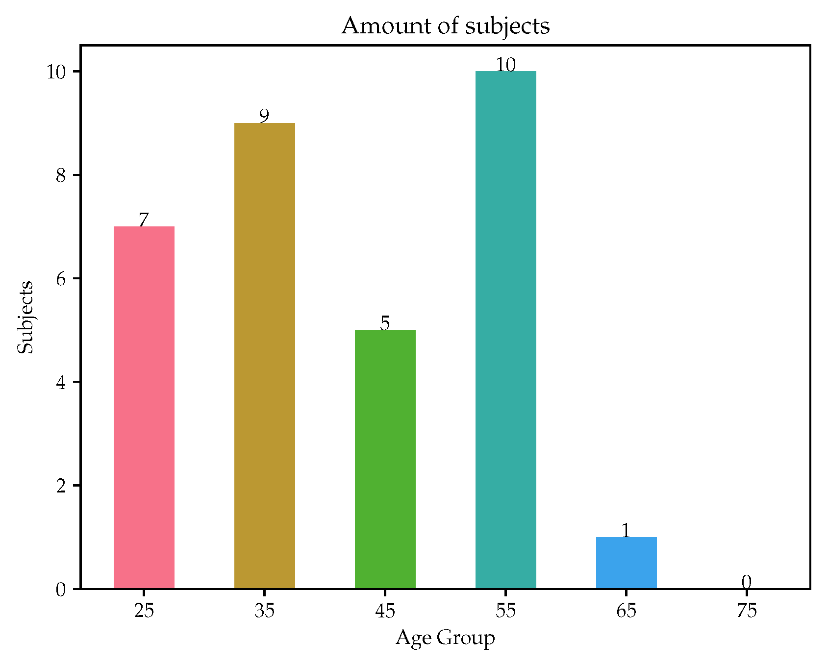
A smaller in vivo dataset was used as a form of validation, including subjects with different health backgrounds and pathologies, from healthy to several preconditions. A total of 32 volunteers were recruited by Universidad de la República, Montevideo, Uruguay. In the initial phase, participants underwent a clinical interview to gather lifestyle habits and personal history information, in which risk factors were perceived. Height and weight measurements were recorded to obtain the Body mass index (BMI), which was considered as another significant risk factor in the study. Medication intake was assessed by asking the subjects about their medication usage, as it was considered as risk factor mitigator, since the type of medication taken was associated with the corresponding risk factor (e.g., a subject with high cholesterol taking medication specifically for cholesterol management). Family history was exclusively evaluated for parents.

Participants were asked to rest in a supine position for 10 min before measuring systolic and diastolic blood pressure (SBP and DBP, respectively) using an Omron HEM-433INT Oscillometric System sphygmomanometer (Omron Healthcare Inc., Hoffman Estates, IL, USA), ensuring alignment of the participant’s arm with their thorax in accordance with the Guidelines of the European Society of Hypertension [13]. BAPWs were acquired using the tonometry technique at a sampling rate of 500 Hz and a 16-bit resolution [14]. Subsequently, the tonometric signals were calibrated based on the assumption of a uniform mean minus diastolic blood pressure value across the large artery tree. Signal processing was performed, similar to that of the in vivo dataset. The age distribution is visualized in Figure 2. This study [14] was approved by an independent institutional review board; all subjects provided their written informed consent before inclusion in the study. Research protocol was carried out in accordance with the Code of Ethics of the World Medical Association (Declaration of Helsinki).

2.4. Frequency Feature Assessment

Frequency domain analysis was employed to extract the features used in this paper [15,16,17] as inputs. Each individual beat obtained from signals was expressed as a finite series in accordance with previous research works [18,19], expressed by

$$x\left(t\right)=\frac{A_0}{2}+\{\sum _{n-1}^{k/2}{A}_{n}cosn\omega t_s+\sum _{n-1}^{k/2}{B}_{n}cosn\omega t_s\},$$

(1)

where $\omega$ represents the angular frequency and $t_s$ represents the sampling time interval. Fourier coefficients were determined for each pulse as

$$A_n=\frac{2}{k}\sum _{s-0}^k{x}_{s}cosn\omega t_s\left(\mathrm{for}n=0,1,\dots ,\frac{k}{2}\right),$$

(2)

$$B_n=\frac{2}{k}\sum _{s-0}^k{x}_{s}sinn\omega t_s\left(\mathrm{for}n=0,1,\dots ,\frac{k}{2}\right).$$

(3)

This facilitated the calculation of the Phase angle (P_n) and the Amplitude of n harmonics (Ah_n) present in each beat spectrum, defined as $A{h}_n=\sqrt{A_n^2+B_n^2}$ and $P_n=arctan(Bn/An)$. To determine the Amplitude proportions (C_n), the formula $A{h}_n/A{h}_0\times 100\%$ was used, considering a range of n values from 1 to 4, since that is the amount of harmonics with representative harmonic amplitude. Additionally, the Coefficient of variation (CV_n) of C_n was determined.

Harmonic distortion (HD) serves as a measure of the BAPW characteristics through Discrete Fourier transform (DFT). By computing the squared magnitudes of the Fourier coefficients ($|A_k{|}^2$) and their complex conjugates, HD quantifies the energy ratio above the fundamental frequency and the energy at the fundamental frequency within the waveform.

$$HD=\frac{{\sum }_{k=2}^6{\left|A_k\right|}^2}{|A_1{|}^2}.$$

(4)

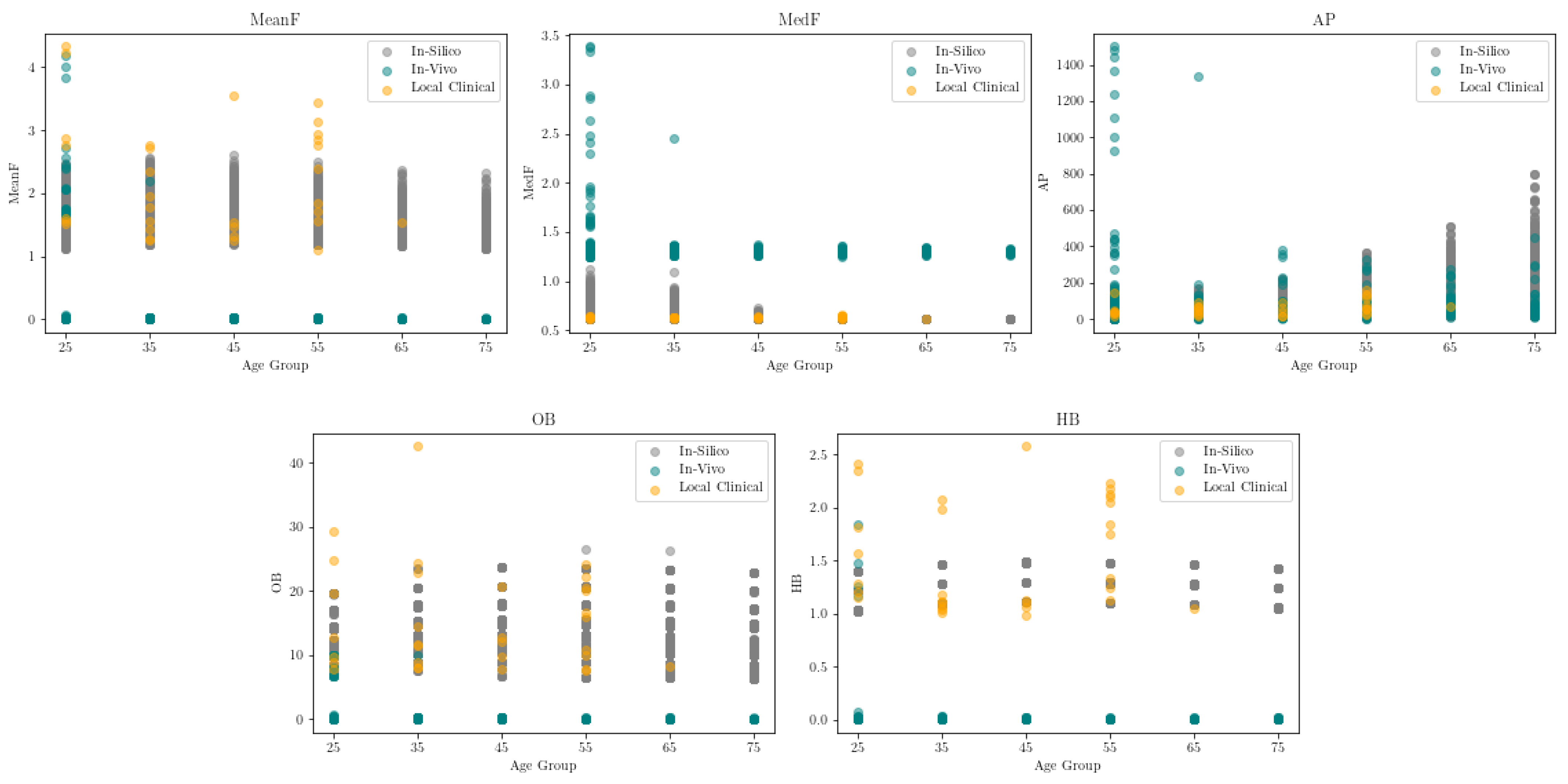
Fourier coefficients beyond the fourth order were disregarded, as they had little influence on the resulting HD value. Finally, Welch’s power spectral density [20] was computed for each individual beat, enabling the extraction of related features, such as Mean frequency of the power spectrum (MeanF), Median frequency of the power spectrum (MedF), Average band power (AP), Occupied bandwidth at 99% (OB), Half-power bandwidth at 3 dB (HB). The Mean and Standard deviation (SD) of each feature was determined. Any values that deviated by more than two SD from the mean for each beat analyzed were eliminated from the signal dataset.

2.5. Supervised Learning Models

In this study, SL was implemented to classify a subject’s vascular age group based on frequency features provided by the BAPW. To further validate the predictive capabilities of the models, an external local clinical in vivo dataset was used. This dataset contained information about each patient’s risk factors and actual age group, providing a reliable ground truth for evaluation.

For the SL models, three widely recognized algorithms were considered, namely Support vector machine (SVM) [21], Random forest (RF) [22] and Multi-layer perceptron (MLP) [23]. These methods were selected due to their proven performance, versatility and broad acceptance in the field. The in silico and in vivo datasets were used for training and optimizing the SL models, which were randomly split into an 80–20% ratio for training and testing, respectively. Then, a ten-fold Cross-validation (CV) strategy was implemented, where, in each fold, one set was separated as the testing group, while the remaining sets served as the training group to fine-tune the model parameters. To obtain the best performance from each algorithm, hyperparameter optimization was performed using RandomizedSearchCV. The hyperparameters for each algorithm were sampled from predefined ranges, which can be seen in

Table 1. List of hyperparameters to be optimized and their range of values.

Model	Hyperparameter	Values
SVM	kernel	[linear, rbf, sigmoid]
	gamma	[0.001, 0.01, 0.1, 1, 10, 100]
	C	[0.1, 1, 10, 20, 50, 100]
RF	n estimators	[500, 700, 1000, 2000, 3000]
	max depth	[5, 10, 20, 50, 100]
	min samples leaf	[5, 10, 50]
	min samples split	[5, 10]
MLP	hidden layer sizes	[(50,), (100, ), (200, ), (50, 50, 50), (50, 100, 50), (100, 100, 100), (200, 200, 200)]
	alpha	[0.0001, 0.005, 0.01, 0.05, 0.1]
	learning rate	[constant, adaptive]

, and the configurations yielding the highest performance metric on the testing sets were selected. This process aimed to achieve optimal model performance while mitigating the risk of overfitting.

2.6. Evaluation

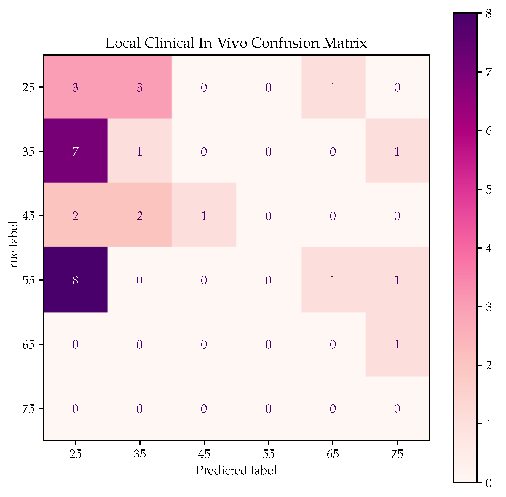
The evaluation of the SL models was conducted to assess their performance and generalization capabilities comprehensively. To achieve this, commonly used classification metrics were employed, such as Accuracy, F1-score, Precision, Recall, Confusion Matrix and Area under the receiver operating characteristic curve (AUC). The AUC metric was evaluated with a “One vs. Rest” approach. Graphics as Confusion Matrix and the Receiver operating characteristic (ROC) curve were evaluated as well.

These evaluation metrics provide valuable insights into the strengths and weaknesses of each model, aiding in making informed decisions about their practical applicability. Additionally, they highlight potential areas for further refinement and improvement, contributing to the development of robust and effective predictive models.

3. Results

3.1. Frequency Features

Table A1. Mean and Standard Deviation ($\mu \pm \sigma$) of Frequency Features extracted from BAPW. HD: Harmonic Distortion. C1–4: Amplitude proportions from first to fourth harmonic. CV_n: Coefficient of Variation. P1–4: Phase angle form first to fourth harmonic. MeanF: Mean frequency of the power spectrum. MedF: Median frequency of the power spectrum. AP: Average band power. OB: Occupied bandwith at 99%. HB: Half-power bandwidth at 3 dB.

Features	In Silico	In Vivo	Local Clinical In Vivo
HD	0.0125 ± 0.0092	0.0085 ± 0.0062	0.0064 ± 0.0038
C1	8.9406 ± 3.3690	6.4252 ± 2.4496	6.0745 ± 1.9122
C2	4.8496 ± 1.1591	4.2977 ± 1.6108	3.6030 ± 1.2904
C3	2.4463 ± 0.5358	2.8972 ± 1.0317	2.1129 ± 0.7930
C4	1.3607 ± 0.4178	1.9138 ± 0.6500	0.9865 ± 0.3579
CVn	199.9370 ± 10.2238	192.8814 ± 13.3849	205.2885 ± 7.2419
P1	−1.7456 ± 0.0898	−1.6587 ± 0.2392	−1.8273 ± 0.2379
P2	−2.2090 ± 0.1594	−2.0939 ± 0.4191	−1.8497 ± 1.3427
P3	−2.4469 ± 1.3432	−0.7413 ± 1.9343	1.7717 ± 1.1535
P4	−2.1248 ± 1.9724	0.9538 ± 1.7368	1.8119 ± 0.7840
MeanF	1.5940 ± 0.3115	6.9438 ± 34.9307	2.1984 ± 0.8949
MedF	0.6343 ± 0.0486	1.3241 ± 0.1601	0.6320 ± 0.0101
AP	81.9902 ± 86.2468	54.0059 ± 126.3425	60.8117 ± 39.8665
OB	12.8854 ± 4.1582	35.0194 ± 125.4401	15.4258 ± 8.0706
HB	1.2651 ± 0.1549	1.7726 ± 8.8819	1.5386 ± 0.5147

shows the feature description, mean and standard deviation values for each dataset. Even though there is a difference between the in silico and in vivo datasets, in terms of mean values and standard deviation, the in vivo dataset displayed a closer resemblance to the in silico one than the local clinical in vivo dataset. Figure 3 presents the values of feature C_n for the first harmonic, highlighting each distinct dataset used. The remaining features can be seen in Appendix A, Figure A1. These features played a crucial role as inputs to the SL algorithms.

3.2. Case Study 1: In Silico Dataset

The study population in Case Study 1 consisted entirely of in silico subjects, a cohort of 4374 simulated individuals. Evaluation metrics for Case Study 1 are presented in

Table 2. Evaluation metrics for Case Study 1. Results from Training CV and In Silico Test Dataset.

Metrics (%)		Models
		SVM	RF	MLP
Accuracy CV		94.45	98.03	95.03
Accuracy Test		96.68	97.60	97.71
F1-Score	25	97.31	95.44	98.64
	35	95.51	95.54	97.16
	45	95.20	97.52	96.55
	55	95.36	99.66	96.34
	65	98.11	98.47	97.72
	75	98.93	99.29	100
Precision	25	96.02	91.82	98.64
	35	97.38	96.77	97.47
	45	93.29	98.57	95.23
	55	95.36	99.34	96.67
	65	98.48	100	98.47
	75	100	100	100
Recall	25	98.64	99.32	98.64
	35	93.71	94.33	96.85
	45	97.20	96.50	97.90
	55	95.36	100	96.02
	65	97.74	96.99	96.99
	75	97.88	98.59	100

. The RF model presented the best accuracy and best performance for the test dataset. However, SVM and MLP showed competitive results as well. Confusion Matrix and the ROC Curve for the best-performing model are shown in Figure 4 and Figure 5.

Subsequently, the RF model was evaluated against both in vivo datasets.

Table 3. Evaluation metrics for Case Study 1. Results from In Vivo and Local Clinical In Vivo datasets. NDA: No Data Available.

Metrics (%)		Dataset
		In Vivo	Local Clinical In Vivo
Accuracy		60.74	15.62
F1-Score	25	77.03	47.06
	35	NDA	12.5
	45	NDA	NDA
	55	NDA	NDA
	65	NDA	NDA
	75	19.84	NDA
Precision	25	65.52	40
	35	NDA	14.28
	45	NDA	NDA
	55	NDA	NDA
	65	NDA	NDA
	75	13.54	NDA
Recall	25	93.46	57.14
	35	NDA	11.11
	45	NDA	NDA
	55	NDA	NDA
	65	NDA	NDA
	75	37.14	NDA

presents the obtained metrics, while Figure 6 and Figure 7 show the Confusion Matrix and the ROC Curve for the in vivo dataset, and Figure 8 and Figure 9 for the local clinical in vivo dataset for the best-performing model. The results from the in vivo dataset revealed a significant bias towards the age group extremes, that is, the 25- or 75-year-old age groups.

Table 4. Distribution of subjects across the In Vivo and Local Clinical In Vivo test datasets based on their VAAG estimation.

VAAG	Datasets
	In Vivo	Local Clinical In Vivo
Higher	84 (7.95%)	17 (53.12%)
Equal	642 (60.74%)	5 (15.62%)
Lower	331 (31.32%)	10 (31.25%)

indicates the amount of subjects from both in vivo datasets that estimated an equal, greater of lower VAAG. The metrics for the local clinical in vivo dataset indicate a less-than-desirable performance, which could be expected given its composition of both healthy and pathological subjects. Nevertheless, it is worth noting a distinct trend towards the 25-year-old age group.

3.3. Case Study 2: Combination of In Silico and In Vivo Datasets

The cohort used for Case Study 2 consisted of both in silico and in vivo subjects.

Table 5. Accuracy comparison between each tested model for Case Study 2.

	Models
	SVM	RF	MLP
Accuracy (%)	87.87	91.82	88.35

indicates the accuracy obtained for each tested model when training with CV. RF once again proved to be the best-performing model.

Table 6. Evaluation metrics for Case Study 2. Results from In Silico and In Vivo test datasets. NDA: No Data Available.

Metrics (%)		Dataset
		In Silico	In Vivo
Accuracy		97.48	66.51
F1-Score	25	95.42	80.61
	35	95.54	NDA
	45	97.52	28.57
	55	99.66	11.76
	65	98.09	40
	75	98.93	40
Precision	25	91.82	68.58
	35	96.77	NDA
	45	98.57	33.33
	55	99.34	50
	65	99.23	75
	75	100	66.67
Recall	25	99.32	97.76
	35	94.33	NDA
	45	96.50	25
	55	100	6.67
	65	96.99	27.27
	75	97.88	28.57

metrics for each individual test dataset are shown for said model. Confusion Matrix and the ROC Curve for the in silico test dataset can be seen in Figure 10 and Figure 11, while those for the in vivo test dataset are shown in Figure 12 and Figure 13, both for the best-performing model.

Table 7. Distribution of subjects across the In Silico and In Vivo test datasets based on their VAAG estimation.

VAAG	Datasets
	In Silico	In Vivo
Higher	29 (3.31%)	22 (10.38%)
Equal	830 (94.85%)	132 (62.26%)
Lower	16 (1.83%)	58 (27.36%)

shows the amount of subjects with higher, lower or equal estimated VAAG. As seen, for the in vivo dataset, for most subjects, an equal VAAG was predicted, while for the in silico dataset, almost for all the subjects, the same VAAG was predicted.

3.4. Validation of Case Study 2

To validate the outcomes of Case Study 2, a population of both healthy and pathological subjects (local clinical in vivo dataset) was implemented.

Table 8. Evaluation metrics from the Local Clinical In Vivo Dataset for Case Study 2.

Metrics (%)		Local Clinical In Vivo
Accuracy		31.25
F1-Score	25	50
	35	25
	45	33.33
	55	37.5
	65	20
	75	0
Precision	25	60
	35	28.57
	45	100
	55	50
	65	11.11
	75	00
Recall	25	42.86
	35	22.22
	45	20
	55	30
	65	100
	75	0

indicates the evaluation metrics for said dataset. Metrics for the 75-year-old class could not be obtained. The underlying reason for this observation becomes apparent when referring to Figure 2, which illustrates that there were no subjects within this particular group. Figure 14 and Figure 15 exhibit the Confusion Matrix and the ROC curve for the RF model.

Table 9. Distribution of subjects across the Local Clinical In Vivo datasets based on their VAAG estimation.

VAAG	Local Clinical In Vivo
Higher	16 (50%)
Equal	10 (31.25%)
Lower	6 (18.75%)

presents the distribution of subjects according to their estimated VAAGs, denoting those with higher, lower or equivalent values. The majority of the subjects had a higher estimated VAAG.

As it can be seen on Figure 16, most of the subjects exhibit at least one risk factor. Figure 17 presents a detailed breakdown of each risk factor individually. Figure 18 shows the distribution of BMI for each subject.

4. Discussion

This study aimed to estimate an individual’s VAAG using SL models based on frequency features obtained from the BAPW. Our findings highlighted the potential of said features as a compelling alternative to temporal and amplitude features, which often require higher sampling frequencies and sophisticated detection algorithms. To begin, one of the main contributions of this study was that frequency features revealed age-dependant variations, displaying either an increase or decrease with advancing age. For instance, the HD feature manifested an augmentation trend with age, while the C_n feature of the fourth harmonic demonstrated a decline. Other features, which appear unaltered by age, suggested that employing dimensionality reduction algorithms could potentially enhance the performance of the SL models applied. Additionally, an integrated dataset encompassing both simulated and real-world subjects was proposed, resulting in significant improvements in model accuracy. Importantly, the use of subjects with risk factors (belonging to a local clinical dataset) for testing purposes contributed to the evaluation of model performance, where differences in VAAG could be expected. This underscores the critical importance of incorporating real-world subject data and considering risk factors to enhance the precision of VAAG estimates, ultimately contributing to more effective preventive strategies and improved cardiovascular health outcomes.

The use of simulated models enables the training of SL models on a larger population and is not dependent on the number of volunteers who can participate. Different health statuses could be simulated, allowing the inclusion of not only healthy subjects but also pathological ones. However, it is worth noting that hemodynamic theoretical values do not always align with those of real subjects, emphasizing the importance of real subject data. A significant variability in these variables from different subjects on similar conditions has been observed [24,25]. In this sense, it is essential to strike a balance between simulation and real-world data, ensuring the models remain grounded in reality. This approach will contribute to more robust and insightful results in the field of healthcare research.

Our findings are in agreement with those of Hsiu et al. [16], as both studies focus on VA estimation using similar frequency features and SL. While Hsiu et al. [16] aimed to discriminate between “Vascular Aging Group” and “Control Group” using binary classification with the Cardio-ankle vascular index (CAVI) as a guide of each subject’s arterial stiffness status, the present study pursued a differentiated classification methodology. A multi-class classification was implemented to estimate VAAG within six different groups, serving as a surrogate of CHA. On the contrary, in this study, multiple SL models were trained with (simulated and real) healthy subjects and subsequently tested with both pathological and non-pathological subjects to detect VA abnormalities. In contrast, Hsiu et al. [16] utilized both healthy and pathological individuals for training. To the best of our knowledge, no other studies have utilized spectrum features for the estimation of VA or other AS indicators.

The findings of Case Study 1 provided valuable insights that justify the need for Case Study 2. The metrics obtained from Case Study 1 demonstrated excellent performance when applied to the in silico subjects. However, when tested on real-world subjects, the results deviated from the expected outcomes. Notably, a significant bias was observed towards the 25- and 75-year-old VAAGs, pointing out a trend to predict extreme values if the subject fell outside the theoretical limits for all features. In contrast, Case Study 2 yielded improved results. 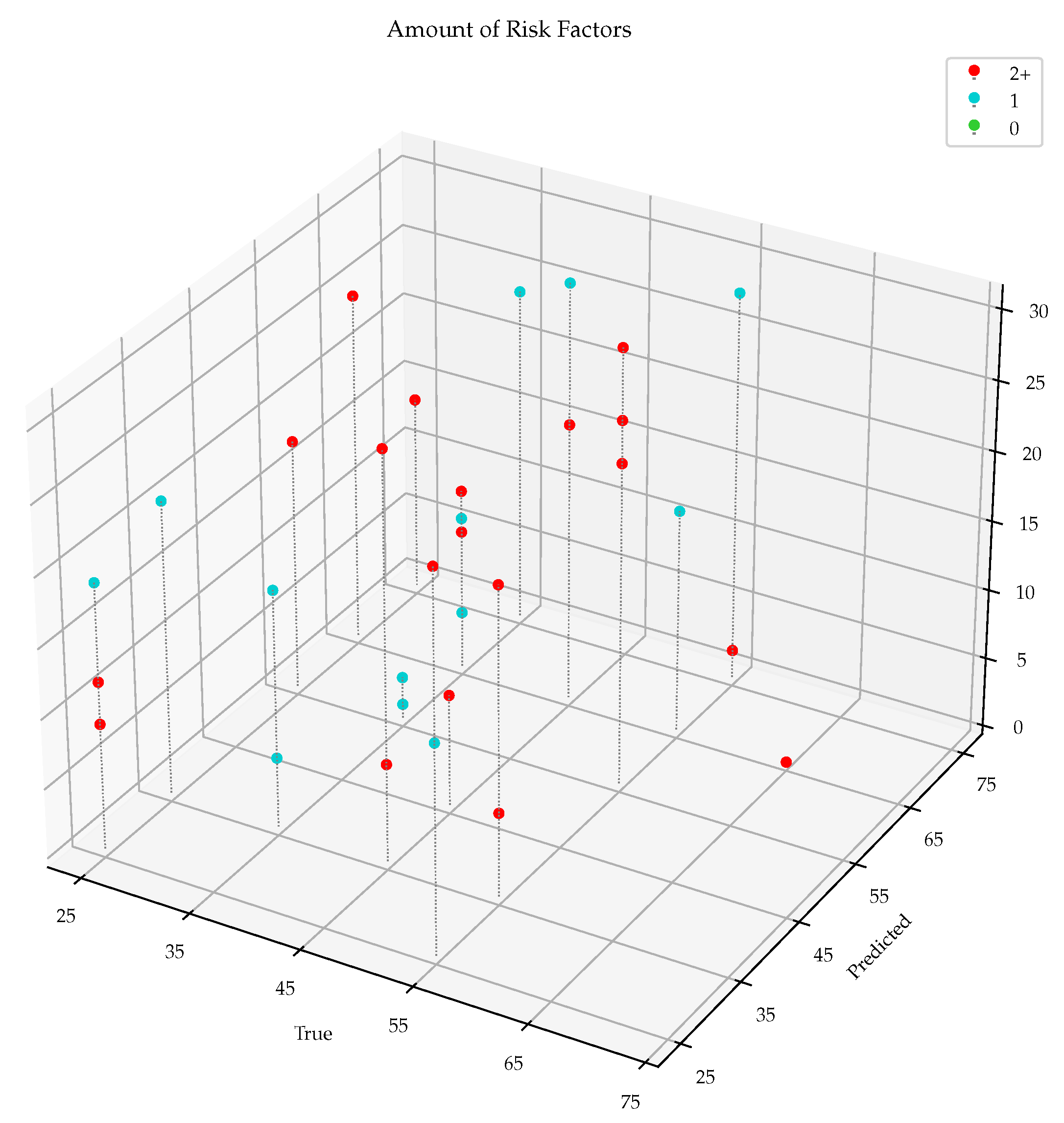However, a bias towards the 25-year-old VAAG was still evident due to the imbalance given by the age distribution of the in vivo dataset (Figure 1) that revealed a predominantly young population, possibly explaining the bias towards the group with a greater number of datapoints. Furthermore, the local clinical in vivo dataset, which mainly comprises pathological subjects, was also tested against Case Study 2 SL models. As was previously mentioned, the metrics were expected to be low due to the fact that the estimated VAAG presented higher values than CHA. Notably, Table 9 demonstrates that the majority of subjects were indeed estimated to have a higher VAAG, aligning with the primary objective of the study.

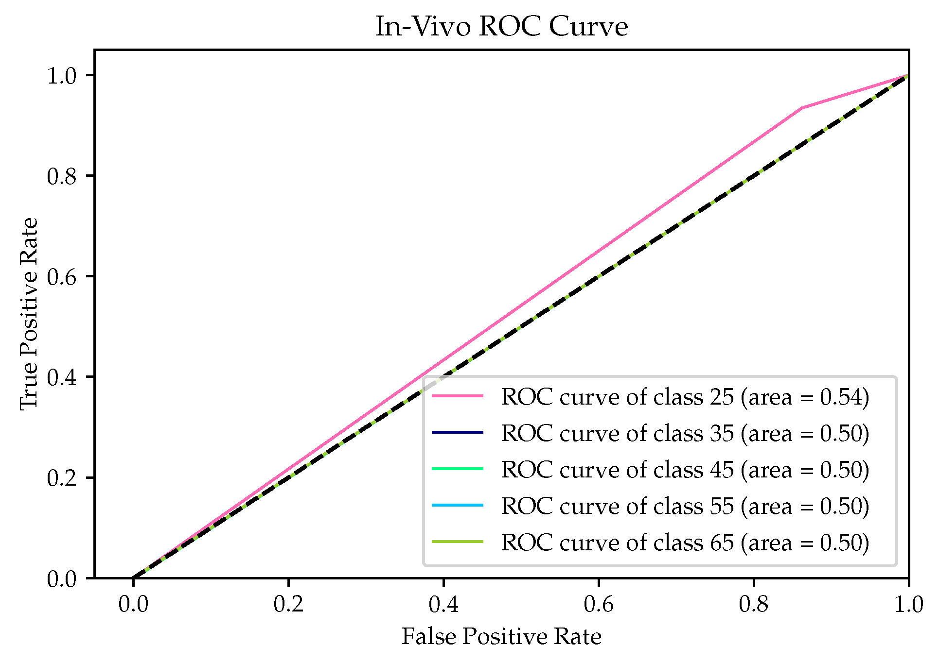
The comparative analysis of SL models, encompassing RF, SVM and MLP, unveiled the superior performance of the RF model, evidenced by its highest accuracy and overall metrics when contrasted with SVM and MLP. This trend is consistent across the two distinct case studies. In Case Study 1 targeting the in silico population, models exhibited metrics closely aligned with exceptional results, as demonstrated by AUC scores approaching unity. However, evaluating the RF model against in vivo measurements revealed limitations due to inherent biases, restricting full class-based evaluation and causing relatively lower metrics, a challenge potentially shared by other algorithms. The ROC curves for the in vivo dataset exhibited complexity. In Case Study 2, the RF model’s superiority strengthened, showing a wider performance gap compared to Case Study 1. Robust performance was witnessed in the in silico dataset, while in the in vivo dataset, inherent bias impacted metric variations across classes. Notably, ROC curves, especially for the in silico dataset, maintained a near-perfect trend, while Case Study 2 curves consistently favored the left side of the central function. When scrutinizing the RF model from Case Study 2 against a local clinical in vivo dataset, AUC scores ranged from 0.87 (highest) to 0.50 (lowest), indicating favorable performance diversity. Overall, these findings underline the RF model’s prowess in addressing bias-related challenges and delivering robust performance across diverse datasets, both simulated and real-world.

The local clinical in vivo dataset was composed by subjects that exhibited one or more cardiovascular risk factors, evidencing that VA could be altered [26]. This observation supports the rationale behind the higher predicted VAAG for the study participants. Notably, a subset of subjects solely presented family history as a risk factor, which could not be considered as a risk group. This subgroup, under normal circumstances, might be overlooked, as they may not present symptoms or conditions. However, given that they could harbor underlying issues that may manifest in 5 to 10 years, this subgroup emerges as a prime candidate for a preventive medicine approach. Targeting this population could potentially yield significant benefits in terms of improving cardiovascular health and overall well-being while addressing potential future health challenges.

A critical challenge in the presented methodology arose from bias, particularly from the in vivo dataset, given its abundance of younger individuals. This imbalance proved to influence the training process, and, in consequence, the results lead to inaccuracies in the predictions. This is acknowledged as a limitation of our study. To address this issue, data augmentation techniques could be employed. Through data augmentation, synthetic BAPW could be generated within underrepresented VAAG, thereby achieving a more balanced dataset. This strategy is designed to enhance the robustness of SL models and improve their ability to generalize, ensuring more reliable predictions across all VAAG. Further data collection would be needed to support data augmentation from several subjects.

For a thorough validation of the proposed approach, it is imperative to have a dataset comprising both control subjects and those with known pathologies. By comparing the predictions of our models against this well-defined dataset, a better understanding of the model performance and identification of potential areas for improvement could be gained. Additionally, the importance of utilizing PWV as a gold standard for precise evaluation of individual vascular health status is recognized. The incorporation of PWV measurements as a reference in future studies would enhance the reliability and clinical relevance of the proposed estimation method.

Future research should focus on conducting a broader real-world validation study. This would involve recruiting a diverse population of both healthy and pathological individuals in different age groups. In this sense, models could be refined to provide a more reliable prediction for individualized risk assessments and early detection of vascular abnormalities. Additionally, it is imperative that future studies incorporate data augmentation techniques to ensure balance in the datasets, especially in cases where certain age groups may be underrepresented. In conclusion, our findings contribute to advancing the field of vascular age estimation and pave the way for more accurate and personalized approaches to cardiovascular health assessment, ultimately supporting preventive measures and improving overall well-being for individuals across different age groups and health conditions.

5. Conclusions

Overall, this study highlights the use of frequency features for the estimation of an individual’s VAAG through SL methodologies. The use of frequency features, which are less dependent on sampling frequency compared to temporal and amplitude features, allow simplification of data acquisition and effective capture of age-related variations. Moreover, the inclusion of One-dimensional cardiovascular models to enhance population quantities proves to be highly useful, but the need to combine it with data from real subjects is important as well to obtain more accurate results. The results are validated using a comprehensive dataset containing information from both pathological and healthy individuals, ensuring the robustness and generalizability of the models. Among the evaluated SL algorithms, the RF model emerges as the most effective in predicting VAAGs, closely followed by the MLP model. This research provides valuable insights into vascular age estimation and contributes to improving preventive strategies and cardiovascular health outcomes.