Convolutional Neural Networks and Feature Fusion for Flow Pattern Identification of the Subsea Jumper

Abstract

The gas–liquid two-phase flow patterns of subsea jumpers are identified in this work using a multi-sensor information fusion technique, simultaneously collecting vibration signals and electrical capacitance tomography of stratified flow, slug flow, annular flow, and bubbly flow. The samples are then processed to obtain the data set. Additionally, the samples are trained and learned using the convolutional neural network (CNN) and feature fusion model, which are built based on experimental data. Finally, the four kinds of flow pattern samples are identified. The overall identification accuracy of the model is 95.3% for four patterns of gas–liquid two-phase flow in the jumper. Through the research of flow profile identification, the disadvantages of single sensor testing angle and incomplete information are dramatically improved, which has a great significance on the subsea jumper’s operation safety.

1. Introduction

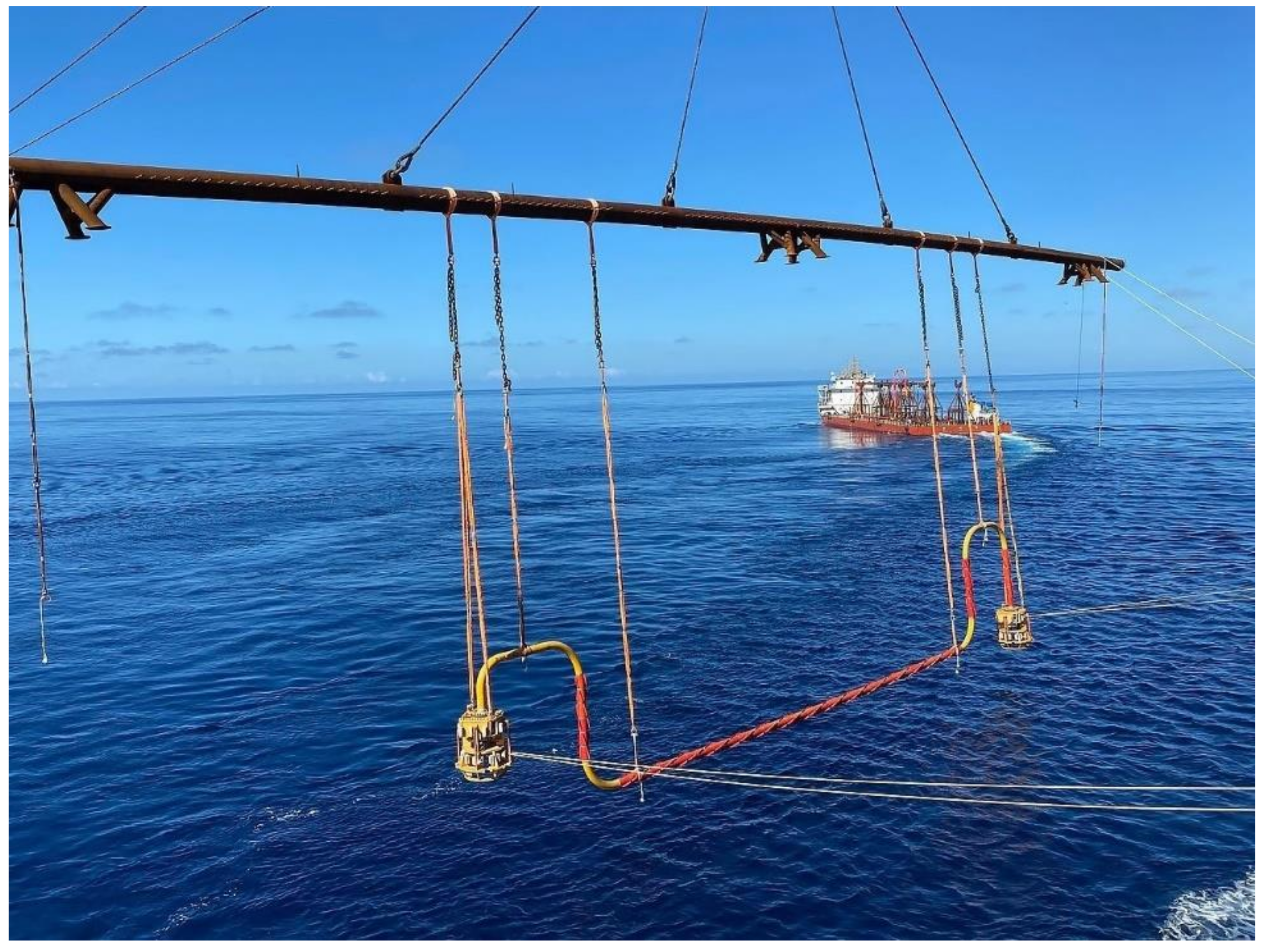
In the subsea production system, a jumper is a pipeline connecting the wellhead, Christmas tree, pipeline manifold, and pipeline terminal, transporting the extracted oil and gas. As shown in Figure 1, a typical M-shaped rigid jumper has multiple bending sections and long overhanging sections. The generation and transformation of flow patterns inside the jumper are closely related to variable gas–liquid velocities, different gas content rates, and pipe shapes and sizes. Stratified flow, slug flow, annular flow, and bubbly flow are commonly seen multiphase flow patterns inside subsea jumpers. The research of flow patterns is essential for understanding multiphase flow characteristics for the design and safety of underwater production systems and operation efficiency. It can also determine the potential dangerous factors and take corresponding protection measures [1]. Therefore, it is important to study how the jumper’s internal flow pattern changes with the flow rate of gas or liquid.

The traditional gas–liquid two-phase flow pattern identification method is simplex and mainly relies on experimental data acquisition, in which researchers obtain flow pattern distribution diagrams of different flow patterns by experimental findings that describe how the flow patterns change and identify them from the practical level. The Baker flow pattern diagram [3] and Mandhane flow pattern diagram [4] are the most representative. However, this method has been gradually eliminated by scholars. As the classification of flow diagrams varies with the subjective perception of scholars and is based on the results of a few different kinds of fluids within a certain range of parameters, the applicability of flow diagrams is conditional. At present, the main flow pattern identification methods are direct observation and indirect measurement [5]. Direct observation methods mainly include the visual method and high-speed camera method. This identification method is individually dependent and it is difficult to form a general identification standard for flow classification when using it. The indirect measurement method is based on data processing and analysis of the actual measurement signals of various extracted characteristics of different flow patterns. Carvalho et al. [6] collected the vibration signals of two-phase flow in a vertical pipe and extracted the signals’ root mean square values and the Pearson correlation coefficients to accurately classify the studied cases. By using electrical capacitance tomography (ECT) based on fuzzy logic, Fiderek et al. [7] were able to determine the flow patterns in vertical pipes and horizontal pipes with inner diameters of 38 mm, 60 mm, and 90 mm. Ma et al. [8] identified five flow patterns according to the flow pattern maps, pressure drop, and power spectral density (PSD) distribution of pressure drop in a bent tube, studied the regularity characteristics of PSD skewness and multiscale entropy (MSE) rate, and the flow patterns in U-shaped tubes were identified objectively. However, this method of identifying flow patterns based on extracting features from sensor signals consumes a lot of time and effort in the pre-processing data stage, which reduces the efficiency of real-time identification.

A flow pattern recognition method based on deep learning has received wide attention. The deep learning model emphasizes the depth of model structure and the importance of feature learning, which can more profoundly depict data-rich information. To collect different photos of oil–water two-phase flow patterns, Du et al. [9] set up an oil–water experiment platform. They used an image segmentation method based on the lowest gray level to extract the characteristics of the flow patterns. To extract image features, three common convolutional neural networks structures were used to identify typical oil–water two-phase flow patterns. OuYang et al. [10] constructed a different deep neural network model. By importing two-phase flow conductivity signals into the bidirectional extended short-term memory network and CNN, considerable signal details were used to understand the depth characteristics of distinct flow patterns. The results show that the model can accurately identify complex flow patterns.

The aforementioned methods only use data from a single sensor and feature extraction of only one source of information, and do not fully utilize the rich understanding of the flow patterns in order to identify the feature fusion flow pattern. This can affect generalization performance of the recognition method, which means it is not fully applicable to different flow patterns. Therefore, the present study uses multi-sensor information fusion (MSIF) for flow pattern recognition to improve the model generalization performance.

Multi-sensor information fusion (MSIF) is widely used in the military [11], medical field [12], fault diagnosis [13], intelligent transportation [14], and many other applications. For flow pattern identification, Toye et al. [15] combined X-ray chromatography imaging and capacitance chromatography imaging, and fused the acquired data to understand and study the gas–liquid distribution of the absorption column at the experimental monitoring point. Hjertaker et al. [16] used a combination of capacitance tomography and γ-imaging systems in their oil–gas–water three-phase flow rate detection study. Combining the two modalities, three-phase rate and flow pattern were obtained.

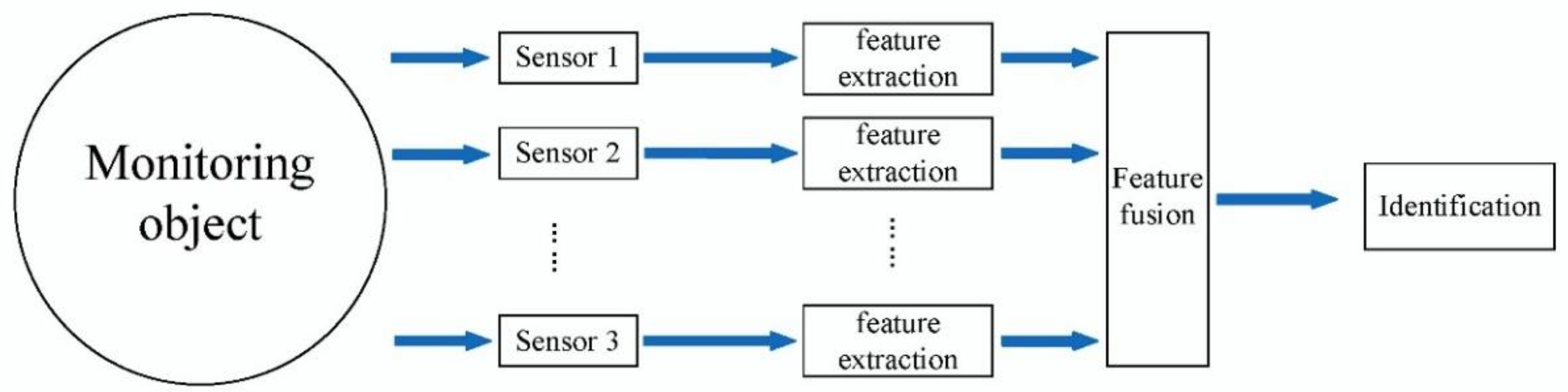
Up to now, data-level fusion, feature-level fusion, and decision-level fusion are the three main focuses of MSIF technology. Data-level fusion directly combines the original data from many sensors. Then feature vectors are extracted from the fusion data set for training and recognition, which requires two kinds of data from the same type of sensors and is computationally intensive. Decision-level fusion processes the data collected by all sensors for recognition, fuses the recognition results, and outputs the total decision results. It is greatly affected by the measurement target and has a high processing cost and the vast elements of the knowledge base. Feature-level fusion (Figure 2) extracts features from the original data measured by each sensor, and then fuses the features extracted by each sensor into a feature vector to identify the target state.

Feature-level fusion technology is the most mature among the three levels of fusion. Since a complete set of proven feature association techniques has been established in feature fusion, the consistency of fused information can be guaranteed. Therefore, feature fusion is chosen as the mode of MSIF in the present research.

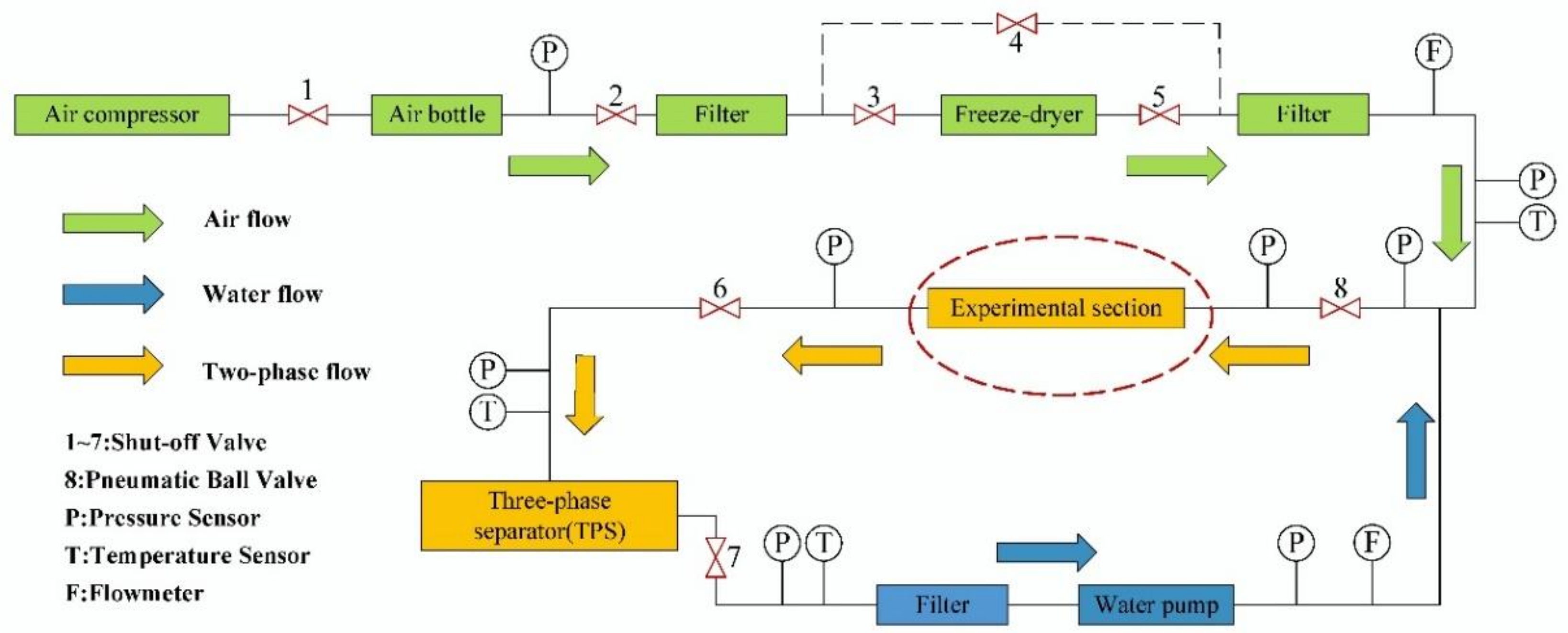
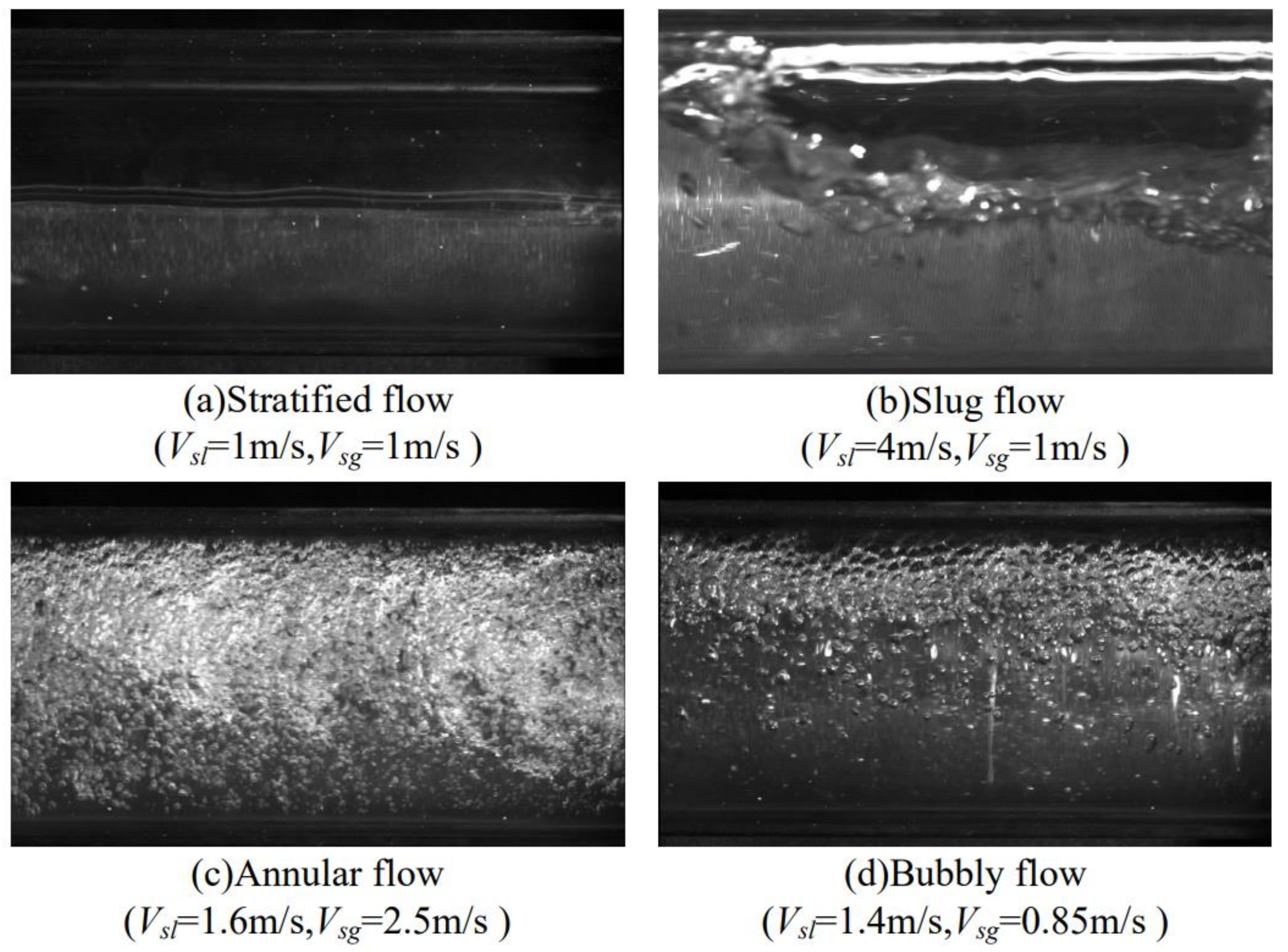
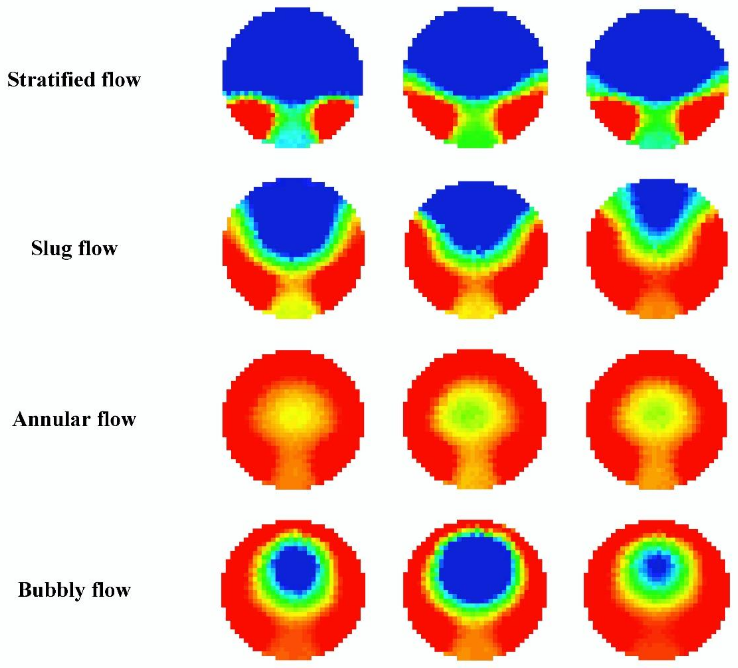
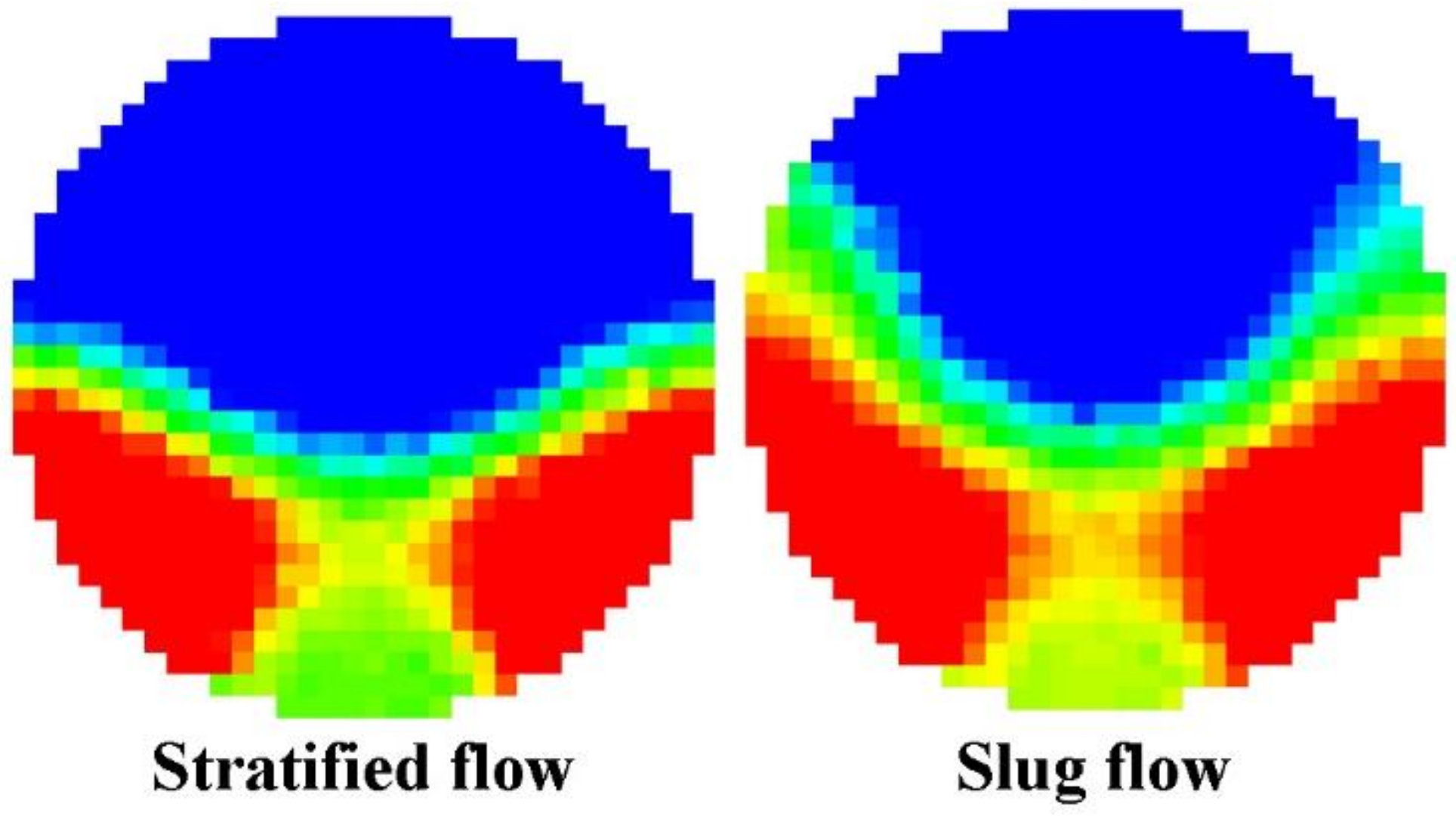
Deep learning has strong learning ability and good adaptability, and the disadvantages of single sensor testing simplex and incomplete information can be solved by multi-sensor information fusion technology. A convolutional neural network can automatically optimize features, remove noise, and obtain features. Therefore, the selected approach for the present work is based on CNN and feature fusion to identify the gas–liquid two-phase flow pattern of a subsea M-shaped rigid jumper. At the same time, the features of the flow vibration signal and capacitance chromatography signal are fused by correlation function. First, the experiment was conducted based on the multiphase flow experimental platform of Dalian Maritime University. Then a vibration signal acquisition system and a tomographic imaging acquisition system were built. Gas–liquid two-phase flow experiments were conducted simultaneously to obtain ECT image data sets and vibration signal data sets for four typical flow types: stratified flow, slug flow, annular flow, and bubbly flow. The convolution neural network structures suitable for signals and images were built to extract the features of two different signals, and the feature fusion was carried out at the complete connection layer. Finally, the integrated features were trained and classified.

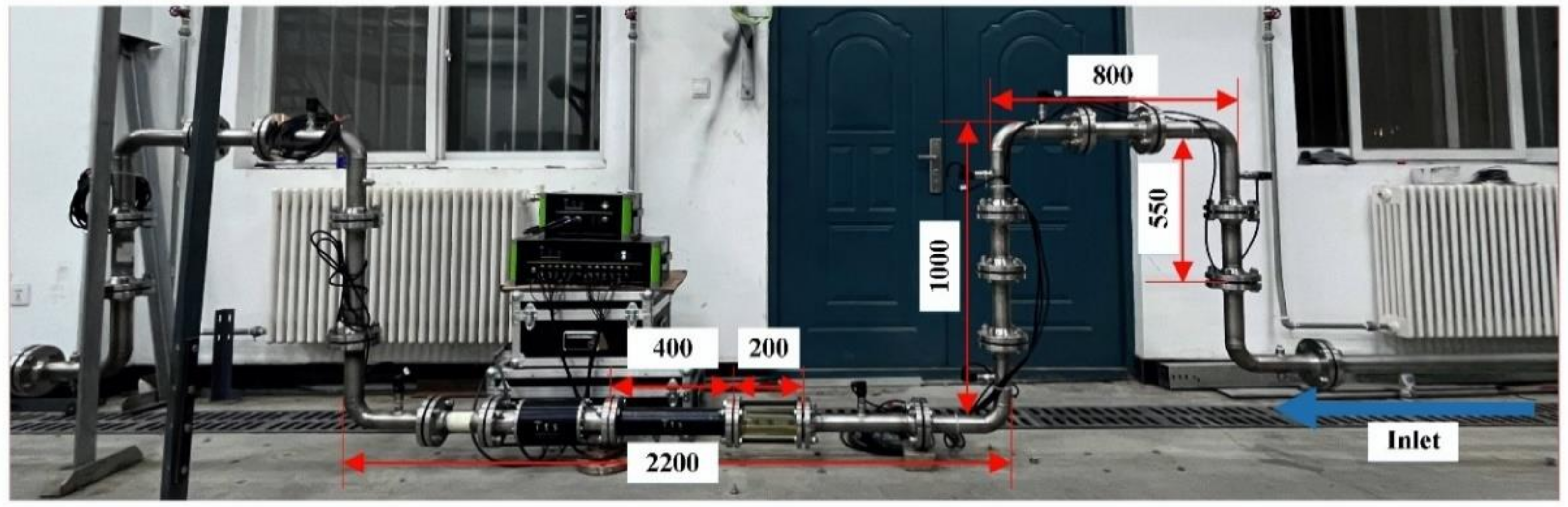
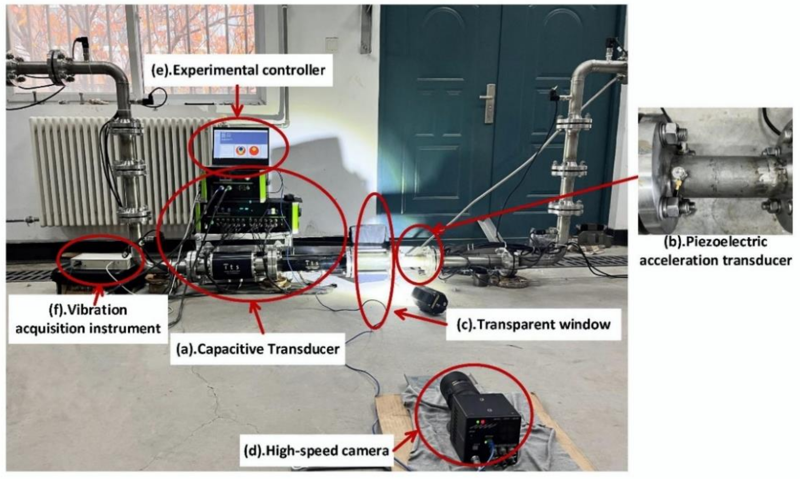
The present study is structured as follows. Section 2 covers the CNN theory, the feature fusion method, the capacitance tomography in, and the structure of the convolutional neural network fusion model proposed in this study. Section 3 presents the experimental setup for multiphase flow, where four flow patterns are obtained in debugging conditions, and their corresponding tomographic images, vibration signals, and high-speed camera images are collected. Section 4 analyzes the experimental findings and compares them to the findings utilizing solely ECT images. The conclusions of this effort are presented in Section 5.

2. Methods

2.1. ECT Measurement Principle

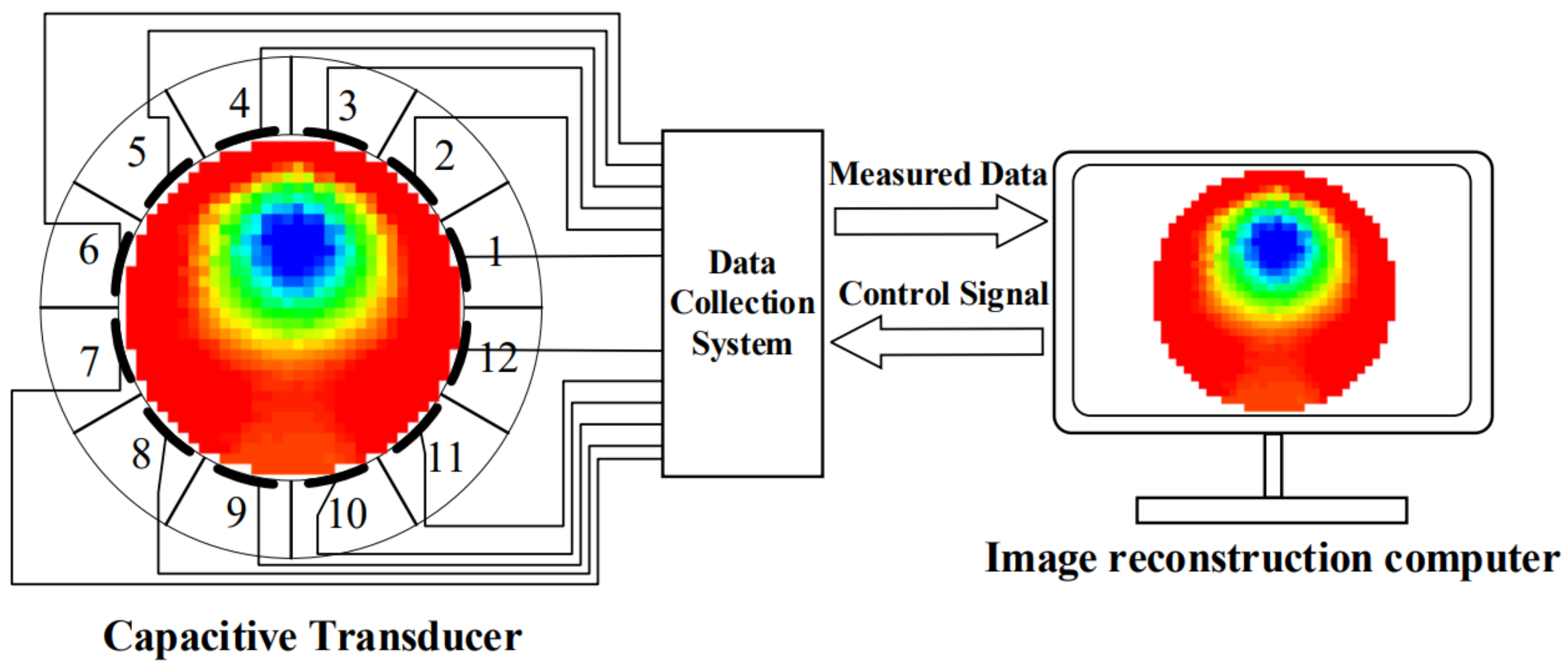
The three primary elements of a capacitance tomography imaging system are a capacitance tomography imaging sensor, a data acquisition system, and an image reconstruction system. A typical 12-electrode capacitance tomography imaging system is shown in Figure 3. The capacitance chromatography imaging system measures the capacitance value inside the closed pipe based on the capacitance sensor array, and transmits it to the computer for secondary calculation after being processed by the data acquisition system, and finally the medium distribution image inside the pipe is reconstructed. The working principle is that when the medium concentration or medium distribution in the measured field changes, the capacitance sensor array detects the change in capacitance value, and the data acquisition system filters, transforms, and amplifies the capacitance value and then transmits it to the computer, which presents the projection distribution in the pipe according to the image reconstruction algorithm.

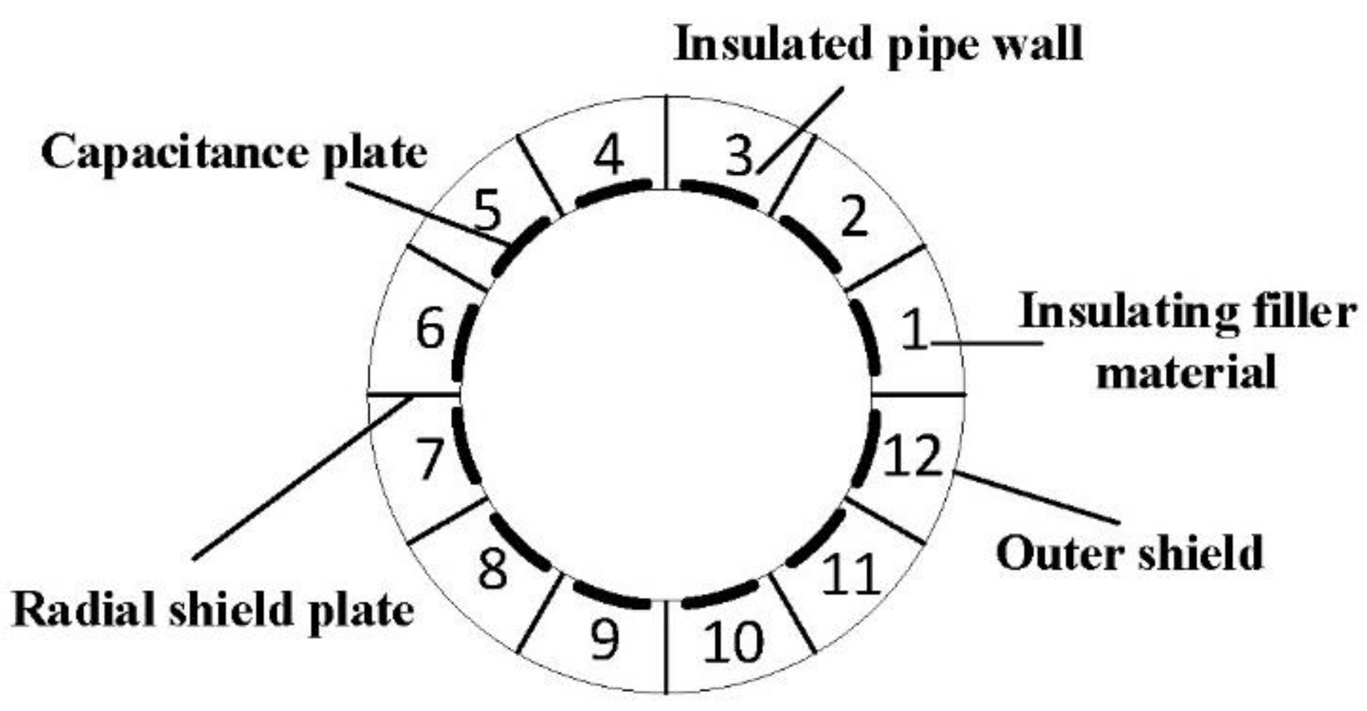
An array of ECT sensors is formed by adding electrodes uniformly on the outside of a multiphase flow pipe and applying electricity to the electrodes in turn to detect the capacitance values between the different electrodes to form the initial measurement data. Most of the current ECT capacitance sensors are 8 electrode, 12 electrode, and 16 electrode. This study is based on a typical 12-electrode ECT system, whose physical structure is shown in Figure 4 in cross-section.

ECT capacitive sensors work with voltage excitation and capacitive output. The conventional single-electrode excitation method is used in this study. The internal electrode number of the capacitor sensor is shown in Figure 4. In general, for an ECT system with N electrodes, M separate capacitance values will be accepted, and it is written as:

$$M=\frac{N(N-1)}{2}$$

(1)

2.2. Mathematical Model of ECT

Assume that the volumes of the discrete and continuous phases of the two-phase flow are $V_1$ and $V_2$ (gas is referred to as a discrete phase in gas–water two-phase flow, and water is referred to as a continuous phase) The discrete phase’s permittivity is equal to ${\epsilon }_1$, while the continuous phase’s permittivity is equal to ${\epsilon }_2$, the discrete phase is uniformly distributed in the continuous phase, and the equation to calculate the equivalent dielectric constant ε as follows:

$$\epsilon =\frac{V_1}{V}\cdot {\epsilon }_1+\frac{V_2}{V}\cdot {\epsilon }_2=\frac{V_1}{V}\cdot {\epsilon }_1+\frac{V-V_2}{V}\cdot {\epsilon }_2={\epsilon }_2+\frac{V_1}{V}\cdot \left({\epsilon }_1-{\epsilon }_2\right)$$

(2)

Thus, its capacitance value can be calculated:

$$C=K\cdot \epsilon =K\cdot f\left(\frac{V_1}{V}\right)=K\cdot f\left(\beta \right)$$

(3)

where the concentration of the discrete phase is expressed as $\beta =\frac{V_1}{V}$. The equation for calculating the capacitance value shows that the phase concentration’s magnitude β is connected to the capacitance value. There is a character constant $K$ that determines the pole plate’s size. The effective area between the pole plates and the separation between the pole plates are some of the characteristics related to it.

Suppose that the pole plate length can be neglected in the axial direction of the tube, the phase distribution of the medium (multiphase flow) is constant in any cross-section of the tube. Ideally, the influence of the sensitivity distribution function on the medium distribution and the influence of the dielectric interference capacitance can be ignored, and the equation of capacitance $C_j$ between any pair of plates in the pipeline is solved by ignoring the influence of dielectric interference capacitance.

$$C_j={\displaystyle \underset{D}{\iint }\epsilon \left(a,b\right)\cdot S_j\left(a,b\right)d_a{d}_b}$$

(4)

where $j=1,2,\cdot \cdot \cdot ,66$, the numbering meaning is as defined above, $D$ stands for pipe section, the dielectric constant of the medium at a particular spot is represented by the medium distribution function $\epsilon (a,b)$ in the pipe section, which represents the sensitivity function within the pipe. $S_j=\left(a,b\right)$ is the sensitivity distribution function of the capacitor. In the 12-electrode ECT system, each pair of poles can measure 66 independent capacitances, represented by a 66-dimensional vector $\left[C_1,C_2,\dots ,C_{66}\right]$, and a sensitivity distribution function is associated with each capacitance value $S_1\left(a,b\right),S_2\left(a,b\right),$ $\dots ,S_{66}\left(a,b\right)$. According to (5), we can obtain Equation (6).

$$\begin{array}{l}[C_1,C_2,\dots ,C_{66}]=[{\displaystyle \underset{D}{\iint }\epsilon \left(a,b\right)\cdot S_1\left(a,b\right)d_a{d}_b,}\\ {\displaystyle \underset{D}{\iint }\epsilon \left(a,b\right)\cdot S_2\left(a,b\right)d_a{d}_b,}\\ \dots \\ {\displaystyle \underset{D}{\iint }\epsilon \left(a,b\right)\cdot S_{66}\left(a,b\right)d_a{d}_b]}\end{array}$$

(5)

From Equation (6), it is clear that the goal of the ECT system’s image reconstruction is known $\left[C_1,C_2,\dots ,C_{66}\right]$ and $S_1\left(a,b\right),S_2\left(a,b\right),\dots ,S_{66}\left(a,b\right)$ to solve for $\epsilon \left(a,b\right)$, and then use the medium distribution to rebuild the original flow pattern’s image.

Among them, one of the earliest and presently most popular basic imaging methods is the linear back projection technique, which is used by this ECT system. It determines the density value at that location in the pipe by adding up all of the projected rays there and then inverting them [17]. The matrix form of the linear inverse projection is shown in Equation (6):

$$g=S^T\lambda$$

(6)

2.3. Convolutional Neural Network

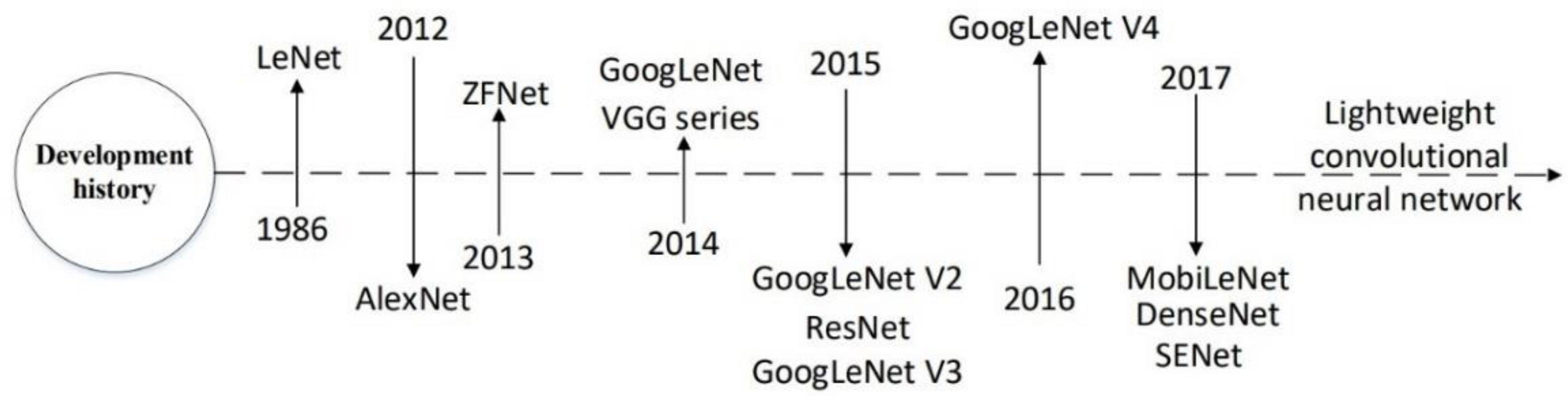
A convolutional neural network (CNN) is an effective feed-forward neural network with complex structure and convolutional computation. LeCun et al. [18] invented the CNN deep learning algorithm in 1998, and the gradient algorithm was used to optimize the model. There are many typical network models, such as LeNet, AlexNet, VGGNet [19], ResNet [20], GoogleNet [21], etc. The development history of network models is shown in Figure 5. In the areas of target recognition, semantic segmentation, and image classification, CNN has so far produced several ground-breaking research findings.

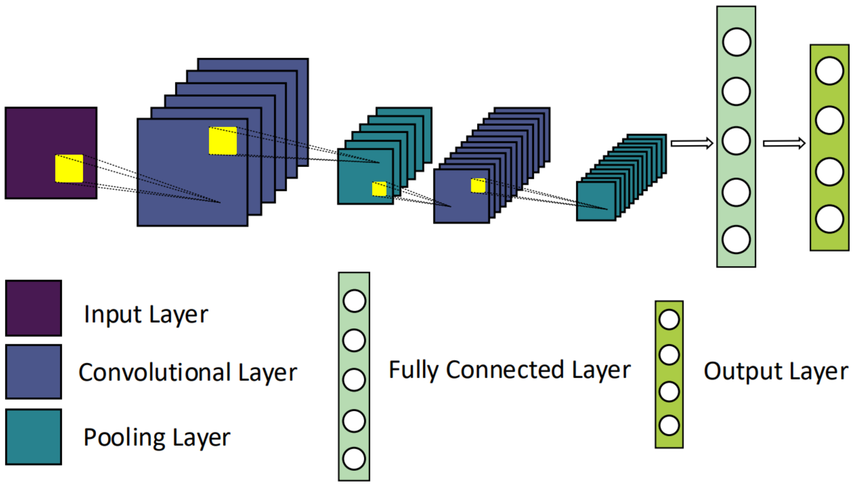
Shared weights, pooling, and sparse concatenation are three ways that CNN differs from other deep learning algorithms (also known as local acceptance domain). It lessens dimensional sampling, lessens the dimensionality of the data in time and space, uses fewer training parameters, simplifies the network, and successfully prevents algorithm overfitting [22]. The classification recognition model of CNN mainly consists of feature extraction of input data through convolutional and pooling layers, classification recognition by combining features and classifiers through fully connected layers. The topology of the traditional convolutional neural network model is represented by the input layer, convolution layer, pooling layer, fully connected layer, and output layer, as shown in Figure 6. Convolutional layer, activation layer, and pooling layer repetition increase the network depth, which is the fundamental element of CNN. The convolutional layer uses multiple convolutional kernels to achieve enhancement, noise reduction, and feature extraction of images using a variety of approaches. The pooling layer, also known as downsampling, speeds up algorithm computation by extracting feature values, reducing the complexity of the computational network, and processing fewer data overall [23]. The basic modules that implement CNN’s feature extraction function are the convolutional and pooling layers [24].

2.4. Feature Fusion

Piezoelectric acceleration sensors and tomography pictures are combined after features are extracted. To this end, we calculated the feature vectors of the data collected by different sensors (i.e., vibration signals and ECT images). We spliced the single feature vectors in the data, which involved the same type in obtaining a new feature vector.

The feature vector is rich in feature information and can better identify flow patterns than the feature vector from information from a single sensor. In feature layer fusion, the key is to balance the feature vectors extracted from multiple sensor data. Multiple feature vectors have to balance in order to allow fused features to have the same numerical scale and length. Therefore, applying the min–max normalization technology [25] to the obtained feature vectors and then joining them to synthesize a single vector is used. This approach aims to modify the individual feature vectors’ value ranges while converting those values into a fresh set of features with the same numerical scale. According to the formula in (7), the min–max normalization strategy preserves the original fractional distribution and converts the values to a standard range [0, 1].

$$a^{\prime }=\frac{a-\min \left(F_a\right)}{\max \left(F_a\right)-\min \left(F_a\right)}$$

(7)

where $a$ is the value to be normalized, $a^{\prime }$ is the normalized value, $F_a$ denotes the function that generates $a$, $\min \left(F_a\right)$ and $\max \left(F_a\right)$ denote the minimum and maximum values of $F_a$ for all possible values of $a$, respectively.

The size of the data feature vector acquired by the piezoelectric accelerometer for each vibration signal data is fixed; conversely, the feature vector of the ETC laminar imaging image is extracted. Firstly, it is necessary to ensure that the two types of signal data set input to the network model are consistent in number and keep the correspondence in the signal. Secondly, the two types of signal data feature sets are convolved, pooled, normalized, and processed through other series of operations to ensure that the feature vectors of the two signal data types have the same length. Finally, the feature vectors are connected for fusion.

2.5. Construction of Neural Network Based on Multi-Sensor Information Fusion

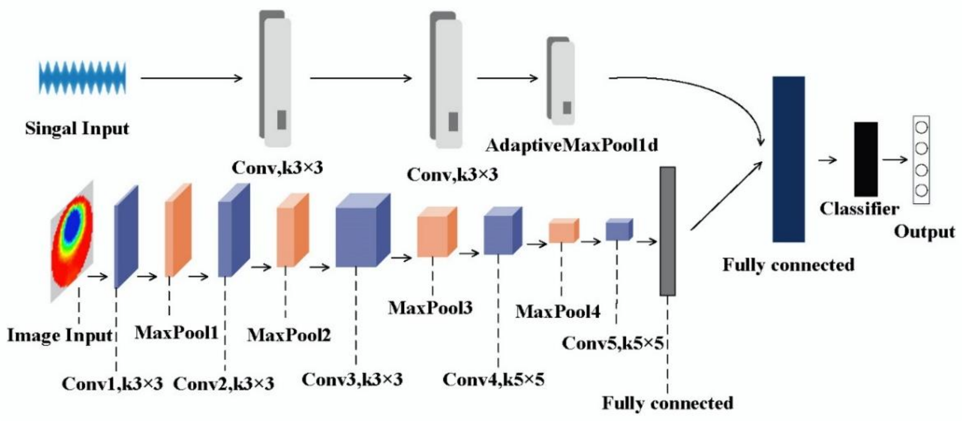
Two channels form the proposed convolutional neural network for flow pattern detection based on multi-sensor information fusion feature extraction of data samples collected by different sensors performed parallelly for the same flow condition, and then the extracted features from each channel are fused to achieve flow pattern recognition across the receiver two-phase flow using a classifier.

The proposed convolutional neural network model for multi-sensor feature fusion is divided into two channels. One channel is used to extract vibration signal features, and mainly consists of two convolutional layers, i.e., an adaptive pooling layer and a flattening layer. The batch normalization (BN), Leaky ReLu activation function, and one-dimensional convolutional module (Conv1d) are all included in the convolutional layer. The other channel is utilized to extract the ETC tomography image characteristics, which consist of five convolution layers, i.e., four maximum pooling layers and one fully connected layer. The convolutional layers include a two-dimensional convolutional module (Conv2d), batch normalization (BN), and ReLu activation function. Subsequently, the vibration signal features under different labels are first fused by concatenating, and then the fused signal features are combined with the picture features, and the flow patterns are classified by the fully connected layer, flatten layer, and sigmoid function. Weight variables that the convolutional neural network learned are trained to perform deep learning on the experimentally obtained data set. Figure 7 depicts the structure of the model. Four neurons represent the four most prevalent flow patterns: stratified flow, slug flow, annular flow, and bubbly flow in the classification layer at the bottom of the model.

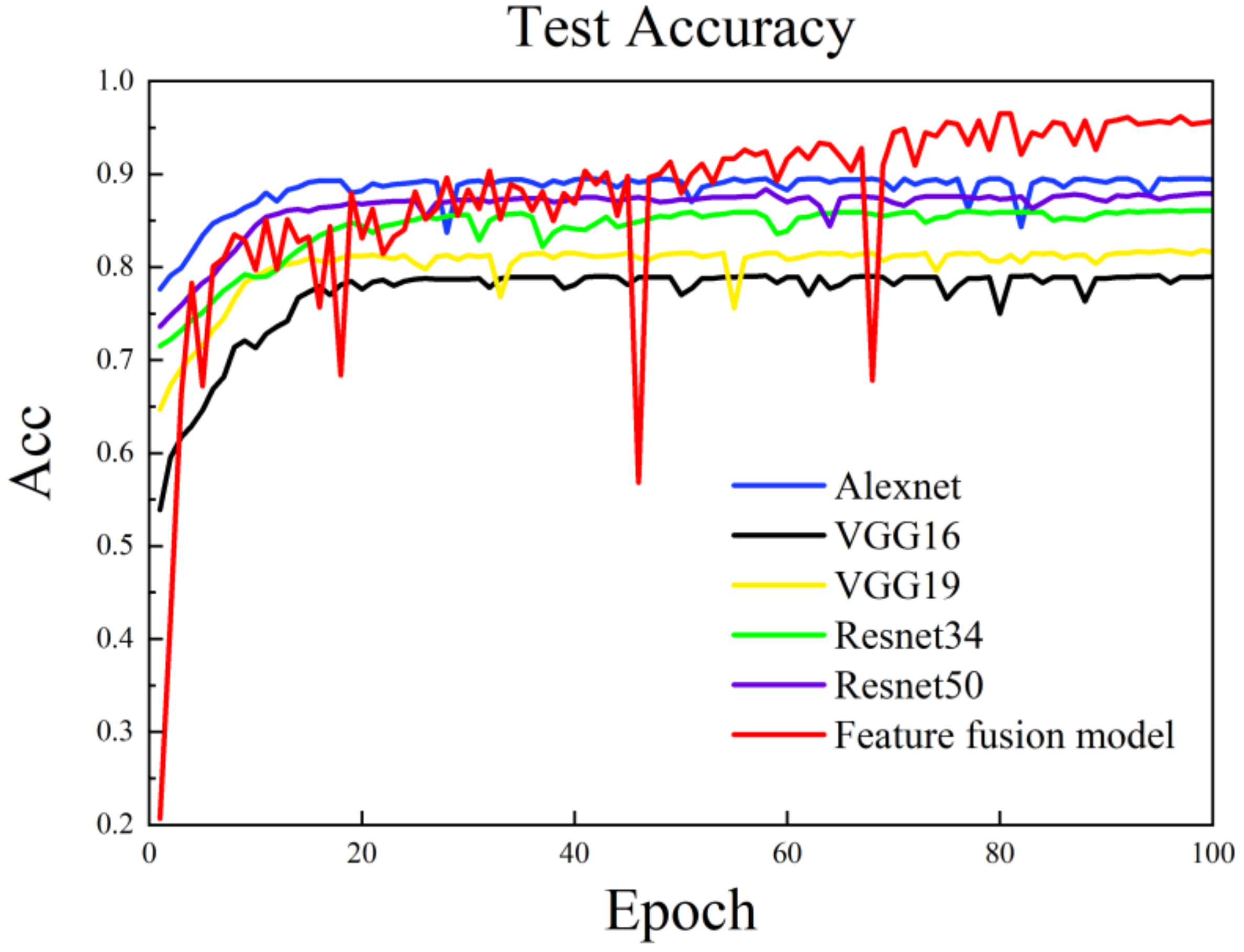
It is found that the multi-sensor feature fusion convolutional neural network model proposed in the subsequent comparison with other models greatly improves the flow pattern identification accuracy of the M-type subsea jumper, and the model has strong robustness, which has engineering application research significance for the influence of flow-induced vibration on the service life of the subsea jumper.

To achieve stream-type recognition, the classification layer employs the sigmoid function as a classifier to determine the probability distribution of successfully identifying various training samples. The following is the formula for the sigmoid activation function:

$$S\left(x\right)=\frac{1}{1+e^{-x}}$$

(8)

The function used as input, the sigmoid function is continuous everywhere, and the data can be compressed with constant amplitude to facilitate forward propagation.

2.6. Evaluation Index

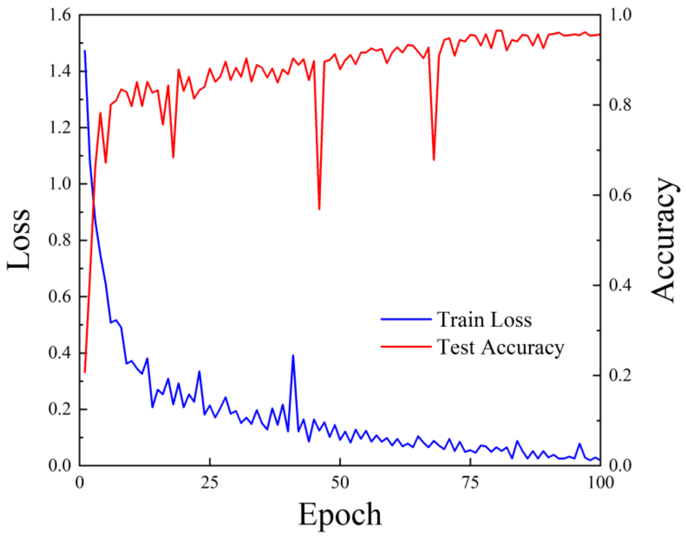
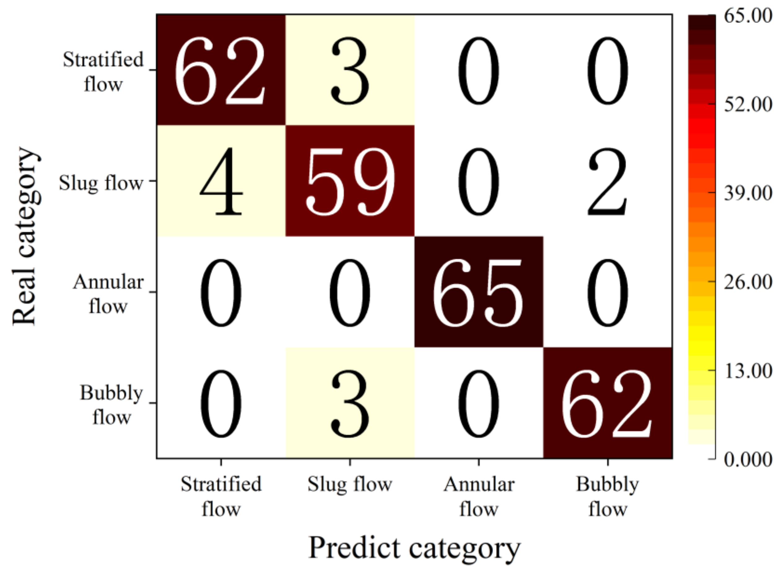
In this paper, loss function, accuracy, and confusion matrix are used to evaluate the recognition results. The loss function curve and test accuracy curve obtained by machine learning training can intuitively understand the recognition accuracy of the model. The confusion matrix compares the real value and predicted value of the fusion sample and visually presents the result through the matrix, so as to measure the robustness of the diagnostic model more comprehensively.

The cross entropy loss function is the loss function employed in this study, and minimizing it is the CNN model’s training target:

$$Loss=-\frac{1}{N}{\displaystyle \sum _{i=0}^{N-1}{\displaystyle \sum _{K=0}^{K-1}{\mathrm{y}}_{i,k}\ln }}{P}_{i,k}$$

(9)

where $y_{i,k}$ denotes the actual label of the ith sample as k, with a total of K label values and N samples, and $P_{i,k}$ denotes the concept of the ith sample predicted as the kth label value. By fitting this loss function, the inter-class distance is also increased.

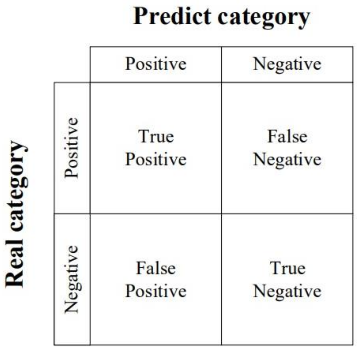
In the field of machine learning, a confusion matrix is a visual tool that is specifically used for supervised learning. In the evaluation of image recognition accuracy, it is mainly used to compare the classification results, as shown in Figure 8. True positive (TP) represents the sample that is actually positive and predicted to be positive; false negative (FN) represents the sample that is actually positive but predicted to be negative; false positive (FP) represents the sample that is actually negative but predicted to be positive; and true negative (TN) represents the sample that is actually negative and predicted to be negative.

Accuracy rate is the most commonly used classification performance index, which can be used to represent the accuracy of a model. The specific expression of accuracy is:

$$A=\frac{TP+TN}{TP+TN+FP+FN}$$

(10)

3. Experimental Setup and Observations

3.1. Multiphase Flow Laboratory

The data set used to train the network for feature fusion to identify flow patterns was provided by the subsea multiphase flow experimental platform at Dalian Maritime University. The modification design of an M-shaped rigid jumper with a pipe with an inner diameter of 50 mm served as the foundation for the experimental platform in the multiphase flow laboratory, and the pipe was constructed of stainless steel 304. The flow pattern information of two-phase flow was collected experimentally, and during the experiment, the fluids that flow in the tube were tap water and air. Figure 9 displays the piping diagram for the gas–water two-phase flow test, Figure 10 indicates the size of the pipeline in the experimental section and the direction of the two-phase flow into the pipeline. The specific dimensions of the jumper are shown in

Table 1. Parameters of the jumper model.

Total Span (m)	Inner Diameter D (m)	Wall Thickness (m)	Radius Of Curvature
3.6	0.048	0.006	1.5 D

. The nominal diameter of the pipe is 50 mm, the inner diameter is 48 mm, and the wall thickness is 6 mm.

The multiphase flow experimental circuit mainly consists of a three-phase separator, two vertical multi-stage centrifugal pumps, flow control valves, air compressors, air bottles, lyophilizer, mixing pipelines, and M-type cross-connections. At the same time, pressure and temperature sensors were installed in each part of the pipeline and test section to monitor the experimental conditions. In the experiment, the medium used for the gas phase was compressed air (density is 1.29 kg/m³, dynamic viscosity is 17.9 × 10⁻⁶ Pa·s). An air compressor with a maximum 20 bar exhaust pressure was available in the lab. After being pressurized by the air compressor, the air enters the air bottle and is transported to the freeze-dryer for drying and processing to reduce the air temperature and prevent its negative impact. Before the compressed air enters the gas–liquid mixing section, the system measures the gas flow rate through the gas mass flow meter. It transmits it back to the control system of the laboratory bench, through which the control system can adjust the gas flow valve to control the gas flow rate. At the same time, the pipeline is also set up with a pneumatic shut-off valve to prevent gas leakage into the pipeline. The medium used for the liquid phase was tap water (density is 998 kg/m³, dynamic viscosity is 0.001 Pa·s), after filtration by the filter, then the water was fed into the experimental circuit by a liquid centrifugal pump. Two vertical multi-stage centrifugal pumps can be operated simultaneously or separately to meet the requirements of different flow rates; the frequency range of the centrifugal pump motor’s frequency conversion is 10 to 50 Hz, the power is 75 kw, the speed is 2970 r/min at rated frequency, the maximum flow rate of a single pump is 998 m³/h after the liquid centrifugal pump is equipped with a liquid mass flow meter, it can gauge the liquid phase’s density and mass flow rate. Using the pump frequency conversion and PID control of the flow control valve, the flow rate can be accurately adjusted to the desired value.

By controlling the ball valve, the gas–liquid two-phase flow runs into the longer extended development section after the air and water have been mixed in the gas–liquid mixing section and form the fully developed flow into the M-type jumper experimental section. After flowing out from the experimental area through the separator return line into the three-phase separator, air flows from the top to the atmosphere or maintains a certain back pressure, water runs into the bottom of the separator and is sent to the test circuit again by the centrifugal pump to achieve circular flow.

3.2. Experimental Facility Setup

The piezoelectric acceleration sensor and capacitance tomography system are installed in the experimental tube section of the multiphase flow experimental loop to obtain vibration signals of different flow patterns and ECT flow pattern images; see Figure 11 for the experimental equipment setup.

The acceleration sensor is a Lance LC0103 with an internal IC piezoelectric accelerometer, which is fixed on the tube wall in order to gather the vibration signal; see Figure 11b. Then the vibration acquisition instrument (Figure 11f) receives the piezoelectric acceleration signal, the signal data are transferred to the host PC via a USB interface, and can be monitored and saved in real-time in the vibration analysis software. These sensors, which combine a piezoelectric acceleration sensor and a charge amplifier, can be linked directly to the recording device, simplifying the test system and enhancing test accuracy and reliability. They also have low noise levels, anti-jamming capabilities, and are appropriate for multi-point measurements.

Table 2. Parameters of Lance LC0103 piezoelectric acceleration sensor.

Sensitivity (mv/g)	Frequency Domain (Hz)	Range (g)	Resolution Ratio (g)	Sensitive Original
50	0.35–10,000	±100	0.0004	Ceramics

displays the acceleration sensor’s specifications.

The ECT flow pattern images were captured and recorded for various flow conditions through the M3C ECT imaging system designed by Industrial Tomography Systems plc (ITS) in the UK, see Figure 11a. The relevant parameters of the M3C ECT imaging system are shown in

Table 3. Parameters of the M3C ECT imaging system.

Operating Frequency (kHz)	Operating Voltage (Hz)	Sensitivity (pF)	Frame Rate (fps)
500	AC sine wave voltage excitation of 18 V between peaks	0.01–1	1–50

. Before the experimental tests, the ECT signal was calibrated to measure the new scalar quantity, and the parameters for scalar quantity acquisition were set in the control system function unit: 0 for measuring low scalar quantity, 1 for measuring high scalar quantity, and 2 for continuous measurement mode. Firstly, to measure the low scalar quantity, it is necessary to ensure that the sensor is empty inside the tube, close the water valve in the multiphase flow laboratory control system, open the air valve and continuously vent the air, and use the three-phase separator to discharge the remaining water from the tube to the water tank. At the same time, the calibration parameter is set to 0 in the ECT system, and the low calibration graph is presented in Figure 12a. Second, the air valve in the control system must be closed to execute the high scalar quantity measurement. It also requires the material with the highest dielectric constant among the testing materials to be used to fill the sensor, and the water valve must be open for water to flow continually through. Meanwhile, the calibration parameter is set to 1 in the ECT system, and what is presented at this time is the high calibration graph, as in Figure 12b. After setting the standard quantification, flow pattern information can be obtained using the ECT tomography system. It should be noted that after the gas–liquid flow setting at the entrance is completed, it is necessary to wait patiently for the flow pattern in the tube to become stable and formed, taking about 1 min, before data collection can be carried out.

In the experimental tube part, as shown in Figure 11c, a clear window with a 220 mm length and an inner diameter matching a plexiglass jumper is placed. A high-speed camera was used as an auxiliary tool to record the flow pattern and flow variations in the tube during the experiment in order to simplify the analysis and validate the experimental data, as shown in Figure 11d. The high-speed camera uses the FASTCAM Mini UX100 from Photron, whose parameters are shown in

Table 4. Parameters of the high-speed camera.

Resolution Ratio	Shooting Speed (fps)	Exposure Time (μsec)	Pixel Size (µm)
1280 × 1024	4000 (full frame) 200,000 (subframe)	3.9	10

.

3.3. M-Shaped Jumper Flow Pattern Information Collection

Based on the multiphase flow laboratory and the signal measurement device shown in Figure 11, the information acquisition of the M-type jumper internal flow pattern is performed. The calibration parameter of the ECT system is set to 2, and the continuous measurement mode is used to acquire ECT images of different flow patterns.

The multiphase flow experiment bench control system controls the gas–liquid velocity by adjusting the gas–liquid flow rate independently or in parallel. For laboratory safety reasons, the gas-phase transition velocity is in the range of 0~5 m/s and the liquid-phase transition velocity is in the range of 0.1~4 m/s. The gas–liquid flow rate is changed while being monitored and controlled in order to achieve the desired flow pattern. Stratified flow, slug flow, annular flow, and bubbly flow are the most common flow patterns to be observed. With thorough mixing of the gas–liquid two phases in the fully developed section, as well as stability checking of the experimental tube section’s flow pattern, the vibration signal was collected using the piezoelectric acceleration sensor as shown in Figure 11b, and data of each flow pattern and each set were collected for a duration of 10 s. Meanwhile, the ECT system (shown as Figure 11a) is used to acquire image data while 1000 sets of signal data and image data are recorded for each flow pattern. In addition, a high-speed camera captures the flow pattern videos for further analysis and verification.

4. Flow Pattern Recognition Results and Discussion

4.1. Data Processing

The high-speed camera’s video recording of the flow pattern reveals that the primary types of flow include stratified flow, slug flow, annular flow, and bubbly flow. Due to the insufficient memory of the high-speed camera system, ECT tomography equipment was used to record and present the flow pattern transformation process. In the M-type jumper, Figure 13 depicts the distribution characteristics of the four gas–liquid two-phase flow patterns. A distinct gas–liquid phase partition interface, also known as stratified flow, can be seen between the gas and liquid phases in Figure 13a when the apparent flow velocities of the liquid and gas phases are preserved at the same value of 1 m/s. The apparent gas velocity remained unchanged, and the apparent liquid velocity gradually increased. During this period, the liquid level gradually increased, but it was still stratified flow, shown by the changes from 1 to 2 in Figure 14. However, it is different from the straight pipe. Under the influence of the complex structure of the subsea jumper and many elbows, there will be a part of the reflux flow pattern, and the stratification cannot be maintained all the time. As the apparent velocity of the liquid increases, a liquid plug filling the entire flow area of the pipe appears, as shown in Figure 14(3). As the apparent liquid velocity eventually reaches 4 m/s, the airflow pushes the liquid wave to the top of the pipe, blocking the entire flow area and causing a blockage. At the same time, because there is a bend across the subsea jumper, liquid flow to the bend forms a flow around, affecting the flow pattern of the monitoring point. Figure 13b depicts the slug flow in place of the stratified flow at this point. The primary characteristic of the gas phase—which takes the shape of a gas elastic in the tube and travels uniformly along the main flow direction with the liquid phase—is its adherence to the top section.

By adjusting the apparent liquid flow rate to 1.6 m/s and the apparent gas flow rate to 2.5 m/s, the flow was stabilized. A layer of the liquid film was discovered to be present along the pipe wall. The majority of the liquid goes forward along the pipe wall as film, as shown in Figure 13c, while the gas rapidly entrains the center of the pipe wall and passes through the pipe as foam. At that point, the flow is annular flow.

Different from bubble flow and slug flow, annular flow is less affected by the structure of the subsea jumper, and the flow pattern remains unchanged basically. The next step is to change the flow of gas and liquid at the entrance into a bubble flow. Gradually reducing the liquid flow and gas flow, we can see from the viewable window that there are some obvious bubbles in the mixture, as the gas phase diffuses into the liquid phase as distributed tiny bubbles. This was discovered by diminishing the apparent gas–liquid flow. Almost all the tiny bubbles are attached to the upper wall surface of the channel. Since the mixture’s average flow rate is low and the bubbles’ rising speed exceeds the liquid flow rate, this flow type is referred to as a bubbly flow, as seen in Figure 13d. From the flow pattern changes of 6 to 10 in Figure 14, it can be seen that the foam in the annular flow is ensnared in the high-speed water flow and appears green in the ECT image. The bubbles in the bubbly flow are larger and more pronounced, and appear blue in the ECT image.

After the steady development of the flow pattern, the ECT tomography system was used to collect about 125 s flow pattern pictures, the frame number was set at 8 fps, and about 1000 flow pattern pictures were collected. The ECT images acquired by capacitance tomography were screened in the ITS Toolsuite equipped with the system, and 650 photos with obvious features, clear images, and less noise were selected from the 1000 data acquired for each flow type. Random sampling was applied to the images represented by every kind of label. The training set to the validation set to the test set ratio was 8:1:1. The ECT flow type samples are shown in Figure 15; these three different transverse images are obtained at different time instantaneous tomography images. According to the strict requirement of the data set for feature fusion above, 650 copies of 1000 sets of vibration signals of each flow type are also selected as a data set. It is not necessary to divide the data set. In the data processing phase, the image and vibration signal data are under the same label. Compared with two-dimensional convolutional neural network, the one-dimensional convolutional neural network has the advantages of small parameter number, easy training, and high computational efficiency. In the model training process, for each image trained, the vibration signal data corresponding to the label of this image will also be trained. The image data sets are divided as shown in

Table 5. Statistical tables for image data sets.

Label	Raw Data Set	Training Sets	Verification Sets	Testing Sets
Stratified flow	650	520	65	65
Slug flow	650	520	65	65
Annular flow	650	520	65	65
Bubbly flow	650	520	65	65
Total	2600	2080	260	260

.

In the process of flow pattern conversion, there are some similar flow patterns in the flow pattern captured by capacitance tomography technology. For example, in the process of flow conversion from stratified flow to slug flow (Figure 14(1–5)), similar flow patterns as shown in Figure 16 appear. At this time, the label definition of the flow pattern needs to be confirmed from the time series of the ECT image. The first flow pattern is named stratified flow, and the second one is slug flow. Then, in the recognition process, the ECT image features of two similar flow patterns become one of the reasons for misjudgment. Secondly, the vibration signal characteristics of similar flow patterns are also similar in the process of flow pattern conversion. Therefore, the eigenvalues that combine two different features make the flow pattern misidentified. In order to avoid misidentification of gender as far as possible, the accuracy of sample labeling needs to be confirmed manually. At the same time, the current excellent Adam optimizer is used to optimize the classification model, which enhances the recognition ability of similar flow patterns in the samples and improves the classification of similar flow patterns.

4.2. Network Training and Results

The training model reads the classified data, and the optimal stream type classification model based on this experiment can be obtained by constantly updating parameters. In the parameter settings, the batch size is 16, with the learning rate set to 0.001, and the number of iterations at 100, while the cross-entropy loss function from Equation (10) is used as the training loss function. Some network parameters of feature fusion are set in

Table 6. Model parameter settings of feature fusion.

ECT Image		Signal
Convolution kernel	[3, 3] × 3 [5, 5] × 2	Convolution kernel	[3, 3] × 2
Max pooling	[2, 2] × 4	Adaptive max pooling	Outsize = 128
Fully connected	[4, 256]	Fully connected	[1, 256]
		Concatenate	[4, 256]
Add		[4, 256]
Fully connected		[4, 256]
Output		4
Epochs		100
Batch size		16
Learning rate		0.001

.

In this study, ECT image data sets with similar flow patterns are affected by each other. It is possible to compensate for the drawbacks of identical flow patterns, increase classification efficiency, and improve classification accuracy by extracting the vibration signal features of various flow patterns and combining them with the flow picture features. The feature fusion model’s training loss and testing accuracy are displayed in Figure 17. The findings demonstrate that the model has a high degree of classification accuracy; within 100 iterations, the test accuracy can reach about 95.3%; and the loss of cross-entropy is reduced to 0.032.

The confusion matrix in Figure 18 demonstrates that the multi-sensor information fusion-based convolutional neural network model can reach 100% accuracy for annular flow. As show in Figure 18, 3 stratified flows were misclassified as slug flow, and 62 stratified flows were correctly identified. A total of 4 slug flows were misclassified as stratified flow, 2 were misclassified as bubbly flow, and 59 slug flows were correctly identified. In addition, 3 bubbly flows were misclassified as slug flows, while 62 bubbly flows were correctly identified.

4.3. Discussion

Traditional flow pattern recognition is subjective, and it is difficult to form a recognized standard for flow pattern classification, and the recognition accuracy is not high. In order to conduct research on flow pattern recognition, more and more experts are now using machine learning approaches, such as neural networks, support vector machines (SVM), random forests, and so forth. The feature fusion recognition approach suggested in this paper was tested to ensure its efficacy. Alexnet, VGG16, VGG19, Resnet34, and Resnet50 classification models in convolutional neural networks are selected for the comparative study of stream type recognition. The data set was selected from the ECT image data that were collected and classified, and only the training learning of images was performed. The data division is shown in Table 5.

The robustness and accuracy of the feature fusion flow pattern recognition model for two-phase flow pattern recognition were verified through comparative analysis, as shown in Figure 19. The recognition results of VGG16 and VGG19 demonstrate that the model’s recognition accuracy really increases with network depth, which is a result of the analysis in Figure 19. The recognition results of Reesnet34 and Resnet50 are also similar. Comparing the model proposed in this paper with some typical classification algorithms, it is found that the feature fusion model has a high flow pattern identification accuracy, which has a significant advantage of 6–17% improvement compared with other single-channel models.

The experimental findings demonstrate the effectiveness of the suggested flow pattern detection approach, and the overall accuracy of the two-phase flow pattern identification for the subsea jumper reaches 95.3%. However, the flow pattern information collected in this study is relatively small. Since the formation of flow patterns depends on different variables, four types of flow patterns, namely, stratified flow, slug flow, annular flow, and bubble flow, may occur under changes in experimental conditions, such as gas–liquid flow rate, gas content, temperature, and diameter of the pipe. To further validate the suggested identification method, more data on the flow patterns across various experimental situations should be gathered in the future.

In addition, the multi-sensor feature fusion method in this study performs direct convolution to extract features from the flow type signal and ECT image. However, it simplifies the feature extraction process and improves the experimental efficiency. It also allows deep mining of the flow type vibration information. The original vibration signal can be subjected to techniques such as FFT and wavelet transform to turn it into a two-dimensional picture. Then, the two-dimensional image features can be extracted and combined with the ECT image data for recognition. By this method, it is verified whether the recognition accuracy can be further improved.

5. Conclusions

This research proposes a multi-sensor feature fusion method for the identification of two-phase flow patterns in a subsea M-type jumper. The experimental tests were conducted at Dalian Maritime University’s multiphase flow laboratory. In the test, flow rates were controlled to generate four different flow patterns: stratified flow, slug flow, annular flow, and bubbly flow. The obtained signals from two different sensing modalities, vibration and capacitive laminar imaging, are used to improve the accuracy issue of single-sensor testing with a single perspective and incomplete information. The proposed model merges their extracted features in a supervised machine learning approach to identify flow patterns. As compared to the model only employing ECT image data to determine flow patterns, the suggested method has a high identification accuracy of 95.3%, according to detailed experimental results.

This study combines machine learning and two different types of sensor information to identify flow patterns, and directly inputs the flow pattern information into the neural network, which simplifies the extraction of features and improves the experimental efficiency. It overcomes the lengthy feature extraction procedure and incomplete feature information in the traditional flow pattern identification approach, which is important for the design and operational effectiveness of underwater production systems as well as the safety.

References

1. Lin, Z.; Liu, X.; Lao, L.; Liu, H. Prediction of two-phase flow patterns in upward inclined pipes via deep learning. Energy 2020, 210, 118541. [Google Scholar] [CrossRef]
2. Li, W.; Song, W.; Yin, G.; Ong, M.; Han, F. Flow regime identification in the subsea jumper based on electrical capacitance tomography and convolution neural network. Ocean Eng. 2022, 266, 113152. [Google Scholar] [CrossRef]
3. Baker, O. Design of pipelines for the simultaneous flow of oil and gas. In Proceedings of the Fall Meeting of the Petroleum Branch of AIME, Dallas, TX, USA, 19–21 October 1953. [Google Scholar]
4. Mandhane, J.; Gregory, G.; Aziz, K. A flow pattern map for gas—Liquid flow in horizontal pipes. Int. J. Multiph. Flow 1974, 1, 537–553. [Google Scholar] [CrossRef]
5. Fourar, M.; Bories, S. Experimental study of air-water two-phase flow through a fracture (narrow channel). Int. J. Multiph. Flow 1995, 21, 621–637. [Google Scholar] [CrossRef]
6. Carvalho, F.d.C.T.; Figueiredo, M.d.M.F.; Serpa, A.L. Flow pattern classification in liquid-gas flows using flow-induced vibration. Exp. Therm. Fluid Sci. 2020, 112, 109950. [Google Scholar] [CrossRef]
7. Fiderek, P.; Kucharski, J.; Wajman, R. Fuzzy inference for two-phase gas-liquid flow type evaluation based on raw 3D ECT measurement data. Flow Meas. Instrum. 2017, 54, 88–96. [Google Scholar] [CrossRef]
8. Ma, X.; Tian, M.; Zhang, J.; Tang, L.; Liu, F. Flow pattern identification for two-phase flow in a U-bend and its contiguous straight tubes. Exp. Therm. Fluid Sci. 2018, 93, 218–234. [Google Scholar] [CrossRef]
9. Du, M.; Yin, H.; Chen, X.; Wang, X. Oil-in-water two-phase flow pattern identification from experimental snapshots using convolutional neural network. IEEE Access 2018, 7, 6219–6225. [Google Scholar] [CrossRef]
10. OuYang, L.; Jin, N.; Ren, W. A new deep neural network framework with multivariate time series for two-phase flow pattern identification. Expert Syst. Appl. 2022, 205, 117704. [Google Scholar] [CrossRef]
11. De Ceglie, S.; Moro, M.L.; Vita, R.; Neri, A.; Barani, G.; Cavallini, M.; Quaranta, C.; Colombi, G. SASS: A bi-spectral panoramic IRST-results from measurement campaigns with the Italian Navy. In Proceedings of the Infrared Technology and Applications XXXVI, Orlando, FL, USA, 5–9 April 2010; pp. 74–86. [Google Scholar]
12. Yadav, S.P.; Yadav, S. Image fusion using hybrid methods in multimodality medical images. Med. Biol. Eng. Comput. 2020, 58, 669–687. [Google Scholar] [CrossRef]
13. Bai, R.; Xu, Q.; Meng, Z.; Cao, L.; Xing, K.; Fan, F. Rolling bearing fault diagnosis based on multi-channel convolution neural network and multi-scale clipping fusion data augmentation. Measurement 2021, 184, 109885. [Google Scholar] [CrossRef]
14. Guo, J.; Zhang, X.; Huang, Z.; Li, B. Autonomous Flight Control Design Based on Multi-Sensor Fusion for a Low-Cost Quadrotor in GPS-Denied Environments. In Proceedings of the 2022 7th Asia-Pacific Conference on Intelligent Robot Systems (ACIRS), Online, 1–3 July 2022; pp. 53–57. [Google Scholar]
15. Toye, D.; L’Homme, G.; Crine, M.; Marchot, P. Perspective in data fusion between x-ray computed tomography and electrical capacitance tomography in an absorption column. In Proceedings of the 3rd World Congress on Industrial Process Tomography, Banff, AB, Canada, 2–5 September 2003. [Google Scholar]
16. Hjertaker, B.T.; Tjugum, S.-A.; Hammer, E.A.; Johansen, G.A. Multimodality tomography for multiphase hydrocarbon flow measurements. IEEE Sens. J. 2005, 5, 153–160. [Google Scholar] [CrossRef]
17. Haijun, L.; Yongping, Y. Improved SIRT algorithm and its application to reconstruct image in underground magnetic CT. Energy Procedia 2011, 13, 5720–5725. [Google Scholar]
18. LeCun, Y.; Bottou, L.; Bengio, Y.; Haffner, P. Gradient-based learning applied to document recognition. Proc. IEEE 1998, 86, 2278–2324. [Google Scholar] [CrossRef]
19. Simonyan, K.; Zisserman, A. Very deep convolutional networks for large-scale image recognition. arXiv 2014, arXiv:1409.1556. [Google Scholar]
20. Wu, S.; Zhong, S.; Liu, Y. Deep residual learning for image steganalysis. Multimed. Tools Appl. 2018, 77, 10437–10453. [Google Scholar] [CrossRef]
21. Krizhevsky, A.; Sutskever, I.; Hinton, G.E. Imagenet classification with deep convolutional neural networks. Commun. ACM 2017, 60, 84–90. [Google Scholar] [CrossRef]
22. Qu, J.; Yu, L.; Yuan, T.; Tian, Y.; Gao, F. Adaptive fault diagnosis algorithm for rolling bearings based on one-dimensional convolutional neural network. Chin. J. Sci. Instrum. 2018, 39, 134–143. [Google Scholar]
23. Zhu, Z.; Peng, G.; Chen, Y.; Gao, H. A convolutional neural network based on a capsule network with strong generalization for bearing fault diagnosis. Neurocomputing 2019, 323, 62–75. [Google Scholar] [CrossRef]
24. Wu, C.; Jiang, P.; Ding, C.; Feng, F.; Chen, T. Intelligent fault diagnosis of rotating machinery based on one-dimensional convolutional neural network. Comput. Ind. 2019, 108, 53–61. [Google Scholar] [CrossRef]
25. Jain, A.; Nandakumar, K.; Ross, A. Score normalization in multimodal biometric systems. Pattern Recognit. 2005, 38, 2270–2285. [Google Scholar] [CrossRef]
Figure 1. Ready for installation of M-shaped rigid jumper [2].
Applsci 13 10512 g001
Figure 2. Feature-level fusion.
Applsci 13 10512 g002
Figure 3. The composition of the ECT system.
Applsci 13 10512 g003
Figure 4. Physical structure cross-section of ECT.
Applsci 13 10512 g004
Figure 5. Network model development history.
Applsci 13 10512 g005
Figure 6. Traditional convolutional neural network model.
Applsci 13 10512 g006
Figure 7. Neural network structure based on multi-sensor information fusion.
Applsci 13 10512 g007
Figure 8. Confusion matrix.
Applsci 13 10512 g008
Figure 9. Multiphase flow experiment loop.
Applsci 13 10512 g009
Figure 10. Size of M-shaped rigid jumper.
Applsci 13 10512 g010
Figure 11. Experimental facility setup.
Applsci 13 10512 g011
Figure 12. ECT calibration measurement.
Applsci 13 10512 g012
Figure 13. Observation of flow patterns with a high-speed camera.
Applsci 13 10512 g013
Figure 14. ECT image of flow pattern change.
Applsci 13 10512 g014
Figure 15. Samples of ECT flow pattern.
Applsci 13 10512 g015
Figure 16. Similar flow patterns of stratified flow and slug flow.
Applsci 13 10512 g016
Figure 17. Training loss and test accuracy of the overall flow pattern of the fusion mode.
Applsci 13 10512 g017
Figure 18. Confusion matrix of flow type classification.
Applsci 13 10512 g018
Figure 19. Results of training several models are compared.
Applsci 13 10512 g019