Research on Efficient Operation for Compound Interchange in China from an Auxiliary Lanes Configuration Aspect

Abstract

Interchanges are the key nodes of the freeway. Due to the existence of weaving behavior, the traffic flow situation is more complicated for small spacing interchanges. Continuous auxiliary lanes are usually used to connect the entrance and exit to form a compound interchange to reduce the interference of weaving behavior. However, when it comes to the design of auxiliary lane forms, China lacks relevant design specifications and research in this area. As a result, there often exists the phenomenon of mismatch between the design form and the traffic volume. In this paper, we took a compound interchange in Xi’an as the research object, proposing four auxiliary lane design schemes and using VISSIM (2022 student) software to establish the simulation model. Additionally, various traffic conditions were simulated through sensitivity analysis. Finally, using the factor analysis method and entropy method, we comprehensively assigned weights to the indexes. By obtaining the weighted scores for various schemes, it became possible to determine the applicability of each scheme under different traffic conditions. The results indicate that the gradient auxiliary lane can be applied to most traffic conditions and has a smaller land occupation than the traditional design, which is an optimization and improvement for the traditional design form.

1. Introduction

With the rapid urban development and subsequent acceleration of freeway construction, there has been a growing number of road intersections, leading to an increased demand for traffic switching. For intersections between major roads, interchanges are often used to reduce conflicts, improve safety, and optimize efficiency. However, the rapid increase in interchanges leads to decreased spacing, especially for the around-city freeway with a shorter total mileage. For example, the Xi’an around-city freeway has a total length of 80.35 km and has 18 interchanges with an average spacing of 4.46 km. Notably, two of these interchanges have a spacing of less than 1 km (Figure 1).

As a key node of the freeway, interchanges play a role in converting traffic and affect the efficiency of the entire freeway [1,2,3]. The driving situation in the diverging and emerging areas of interchanges can be complicated. When drivers exit a freeway, they are required to perform various tasks, including identifying exit signs, waiting for suitable vehicle gaps, changing lanes, and reducing speed to exit [4]. These diverging actions can increase driving workload and the probability of errors [5,6]. Changing lanes becomes more challenging for drivers when there is high traffic volume, a significant number of freeway lanes, or when trucks in the outer lane create a barrier effect [7]. In the emerging area, there are also accidents, such as collisions caused by insufficient gaps when the driver accelerates into the mainline [8]. Therefore, the entrances and exits of interchanges are recognized as accident-prone areas, with significantly higher accident rates compared to other sections of freeways [9]. In addition, according to relevant statistics, the accident rate in the diverging area is the highest [9,10].

Due to the unique operation mode of interchanges, vehicular behavior exhibits notable deviations from that observed on the basic mainline sections. Therefore, over-intensive interchanges will significantly impact the operational condition of vehicles. However, the limitation of distance should not impede the development of freeway construction. In order to solve the problem of spacing between interchanges, the most efficient solution is to connect two interchanges. The widely adopted method is to connect the interchanges with auxiliary lanes or collector–distributor lanes. However, in China, land restrictions are relatively strict, and the implementation of collector–distributor lanes will occupy more land. As a result, auxiliary lane connections are predominantly used for small spacing interchanges in China. To achieve this, additional lanes are incorporated outside the outermost lane, connecting the entrance and exit ramps. This configuration forms a compound interchange, effectively shifting the weaving behavior to auxiliary lanes. As a result, the normal flow of the mainline straight traffic remains unaffected.

This paper collects traffic volume data from a typical compound interchange in Xi’an. We select four auxiliary lane forms for modeling, calibration, and simulation in VISSIM, using eight indexes of delay, mainline travel time, CO emissions, fuel consumption, number of conflicts, TTC, PET, and CSI as evaluation indexes. Finally, based on the factor analysis method (FAM) and entropy weight method (EWM), the auxiliary lane forms are compared under different traffic volumes, diverging, and emerging rates. The EWM is a method of comprehensive evaluation by assigning weights to different indexes. The EWM has a wide range of applications in many fields, such as environment [11], physics [12], and transportation [13]. The FAM is a method to explore the hidden relationship of several variables and then extract common factors and obtain the optimal solution. The FAM is extensively utilized in the transportation field [14], including identifying the factors affecting accidents in freeway construction areas [15], predicting the severity of freeway accidents [16], and researching road factors that lead to the use of mobile phones while driving [17].

Currently, the configuration of auxiliary lanes connecting interchanges lacks uniformity in China. The relevant norms and standards do not provide specific guidelines, and the design of auxiliary lane configurations lacks reliable research. However, the form of auxiliary lanes significantly impacts efficiency, safety, and construction costs. Therefore, this article aimed to examine the impact of various auxiliary lane designs on traffic efficiency and safety. The aim was to find the best design form that suits various traffic situations.

The remaining sections of the article are organized as follows. Section 2 provides a review of relevant studies. Section 3 states the existing problems and the data collection of the research object. Section 4 presents VISSIM modeling, calibration of the model, and analysis of the results for different types of auxiliary lane forms. Section 5 performs a sensitivity analysis of different schemes under different traffic combinations. Section 6 presents a comprehensive evaluation of the different schemes using the FAM and EWM (FAEWM). Section 7 draws conclusions.

2. Literature Review

2.1. Problems in Small Spacing Distance Interchange

An interchange is an area with a high incidence of accidents, and when interchanges are dense, more problems will arise. In the process of diverging and emerging, the impacts will extend to a certain distance upstream and downstream. The research found that the diverging impact area ranges from the diverging point to 1000 m upstream, and the emerging impact area is from the emerging point to 350 m downstream [6]. Therefore, when the interchange spacing is small, the diverging influence area at the downstream interchange exit will overlap with the emerging influence area at the upstream entrance. This overlap creates a complex traffic environment [18]. Generally, exit signs are set 0.5 km, 1 km, and 2 km before freeway exits. When the interchange spacing is small, the cue signs for different ramps will overlap, leading to difficulties in information recognition for drivers. As a result, vehicles tend to concentrate on changing lanes near the exit [19].

In addition, a major factor that seriously affects traffic efficiency is the weaving behavior of vehicles when the spacing between interchanges is small. The part between the entrance of the previous interchange and the exit of the next interchange creates a weaving area where vehicles change lanes with increased frequency. As a vehicle needs to exit the freeway, it typically needs to transition to the outermost lane in advance. This lane-changing process can have a significant impact on some aspects, including the distribution of vehicles, operating speed, and headway. When vehicles are affected by lane-changing behaviors, they become more vulnerable to traffic accidents [20,21]. Different weaving distances significantly impact accident rates, with short weaving areas having become accident-prone zones [21]. Increasing weaving distances can improve the driving environment when drivers change lanes continuously, thus reducing the frequency of collisions [2].

By studying the operational characteristics of vehicles in the weaving area, it has been observed that most lane changes occur within the initial half of the weaving area or even change lanes immediately after entering the weaving area; the weaving area is not fully utilized, resulting in serious traffic congestion [22,23,24]. From the perspective of traffic psychology, drivers who need to exit will change lanes as soon as possible after entering the weaving area. This behavior is driven by the desire to avoid missing the exit due to a delayed lane change. Moreover, as traffic volume increases, so does the level of psychological tension and urgency experienced by drivers. This leads to the concentration of vehicles changing lanes in the weaving area. The weaving area becomes a bottleneck section because of the diverging and emerging behaviors, which affect the operational efficiency of the freeway. Even in situations with low traffic volume, the weaving area tends to exhibit poor operating conditions [25]. Therefore, by distributing lane-changing behaviors evenly within the weaving area, congestion and safety problems caused by concentrated lane-changing can be effectively improved [26].

Currently, traffic volume is increasing rapidly, and freeways are facing or have completed reconstruction and expansion projects to accommodate the growing demand by increasing the number of lanes. For small spacing interchanges, it is more difficult for vehicles to change lanes. Drivers are unable to find a suitable gap for lane changes before the diverging area, resulting in forced lane changes or even stops close to the diverging point. As a result, this leads to a significant increase in traffic conflicts. It has been found that the main cause of accidents occurring in the weaving area is attributed to forced lane changing. This behavior becomes particularly prominent when the interchange spacing is too small [4]. It is worth noting that this hazardous behavior tends to occur near exit ramps. In a section with a small spacing between the tunnel exit and the interchange exit, when the spacing is less than 500 m, there will be continuously forced lane-changing behavior in the exit section [27].

2.2. Small Spacing Interchange Improvement Methods

Several scholars have investigated the relationship between ramp entrance–exit spacing and freeway accident rates, and the results have shown that the accident rate increases as the ramp spacing decreases [28,29]. It has also been suggested that entrance ramp density has a greater impact on freeway accidents, whereas the effect of exit ramp density is not statistically significant [30].

Current research on interchange spacing is dominated by ramp geometric design and ramp spacing studies. Some scholars have given ramp spacing recommendations for two different ramp combinations: “entrance–exit” and “exit–exit” [31]. Through theoretical derivation and simulation, Liu proposed the spacing between tunnel exits and interchange exits according to varying traffic volumes and diverging rates and comprehensively evaluated the traffic efficiency and pollutant emissions of different schemes based on entropy [32]. Based on a data envelopment analysis combined with a hierarchical analysis, the optimal spacing is proposed for the four ramp combination types of exit and entrance [33]. A scholar has comprehensively considered multiple aspects, such as safety, accessibility, and cost, and developed a dual-objective optimization model for optimizing the layout of highway interchanges [34]. Ma proposed the entropy-weighted TOPSIS evaluation method to study the reasonable spacing between interchanges from four aspects: traffic efficiency, safety, accessibility, and economy [35]. Zhang conducted an analysis of the impact of entrance and exit ramps on the mainline from a mathematical perspective based on the theory of linear stability. They proposed a traffic grid model to study this phenomenon [36]. In order to improve traffic safety in sections with dense spacing between entrance and exit ramps, many scholars have focused on controlling the spacing between ramps based on traffic volume. However, Zhao took a different approach by focusing on improving geometric design. They studied the impact of lane configuration, number of through lanes, spacing between ramps, shoulder width, and other factors on enhancing traffic safety [37]. Huang conducted research on the variation pattern of lane-changing distance with changes in traffic volume and diverging ratio. The author found that for every 100 pcu/h increase in traffic volume per lane, the lane-changing distance should be increased by 50–100 m. The research findings provide valuable insights for the design of interchange spacing [38].

In order to improve the operating conditions in the weaving area, lane utilization and traffic efficiency can be effectively improved by installing continuous auxiliary lanes between the ramps [39] and reducing the accident rate. However, the safety benefits of installing auxiliary lanes tend to decrease as the ramp spacing increases [28,40]. For compound interchange, the safety of type A, B, and C weaving areas is evaluated by building a collision prediction model. The prediction results show that the C-type weaving area exhibits the highest level of safety, and the B-type weaving area has the lowest [2,18].

In addition, it has been found that although a decrease in ramp spacing leads to an increase in collision frequency, drivers will appropriately reduce their speeds in order to avoid an insufficient lane change distance. This adaptive behavior by drivers helps mitigate the severity of collisions [40]. Qi concluded that operating conditions could be effectively improved by extending the auxiliary lanes between the entrance and exit ramps outside the weaving area [41].

Some scholars have also proposed methods of managing interchange hazardous areas using signage and markings. The downstream sections of urban interchanges with short weaving areas were found to be high-risk. The traffic conditions in the high-risk sections were optimized by shifting the traffic risk to areas with better operating conditions. This was achieved by implementing a policy that permitted only vehicles on the outer and auxiliary lanes to change lanes inward near the exits [21,42]. Wang developed a regression model to explore the accident characteristics of small-spacing interchanges based on the number of accidents counted [43].

Sustainable development has been pursued in terms of road design. Some scholars have reduced pollutant emissions and improved congestion and air quality by improving traditional intersections [44,45,46]. Xie believes that improving the capacity of the road itself is the most effective way to relieve congestion [13]. Therefore, there is a need to propose a feasible and efficient form of auxiliary lanes for compound interchanges, which can be used to improve traffic congestion and automobile exhaust pollution.

2.3. Summary

The literature review indicates that current research on small-spacing interchanges predominantly centers around spacing control, primarily serving as a guide during the design stage. When the conditions are restricted, such as the spacing below the standard value or inadequate spacing caused by new interchanges, the utilization of continuous auxiliary lanes becomes necessary. However, there are few studies on the optimal form of auxiliary lanes, and no specific design guidelines exist based on a theoretical foundation.

Reasonable design for auxiliary lanes can improve traffic efficiency and significantly reduce pollutant emissions, minimize land usage, and save costs. Therefore, it is necessary to assess the suitability of different auxiliary lane forms under different traffic conditions and evaluate their impact on operational efficiency and safety. In this study, several evaluation indexes were selected to investigate different forms of auxiliary lanes, and the FAEWM was used to make a comprehensive comparison.

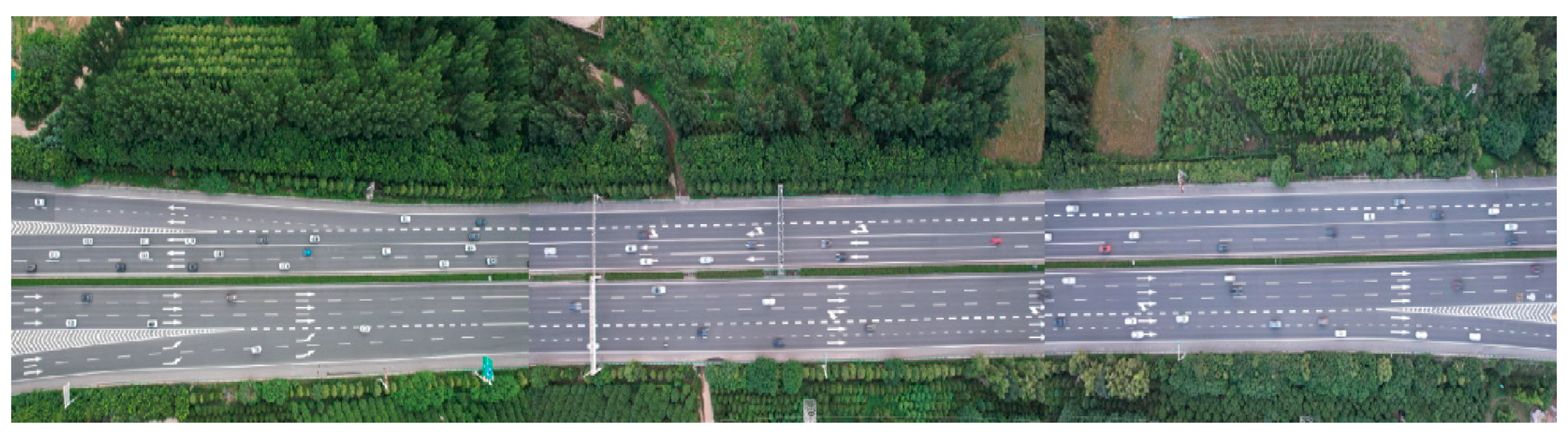
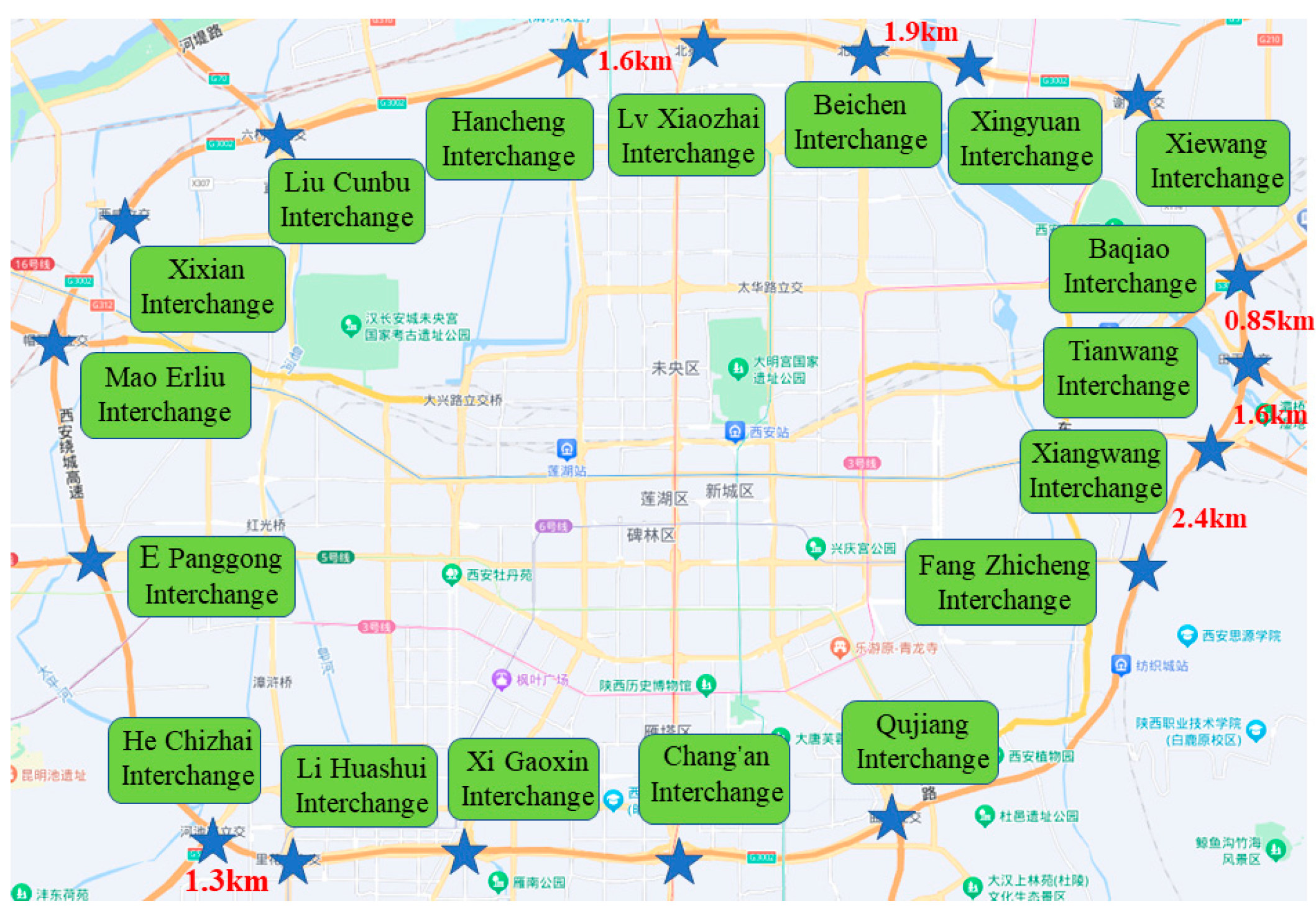
3. Problem Statement and Data Collection

3.1. Problem Statement

Due to complex traffic conditions at the diverging and the emerging area, the impact radiation area is large. Therefore, in order to avoid the mutual influence between interchanges at the early stage of construction, all countries have made relevant regulations on the minimum spacing of interchanges [47,48].

In the initial stage of freeway construction, when the freeway network is relatively sparse, and the spacing between interchanges is significant, it is feasible to design the interchanges as independent units. However, with the development of road transportation and the demand for freeways increases, the intersection of two freeways leads to more interchanges. For example, the construction of the Xi’an around-city freeway and the outer-ring freeway, accessing the surrounding national freeway network, has generated many nodes requiring interchange construction. At this time, if the new interchanges and existing interchanges are too close to each other, resulting in the mutual influence of traffic flow, it constitutes a compound interchange.

However, the relevant specifications in China do not specify the design form of compound interchange auxiliary lanes. Research in this field has primarily focused on the width of the auxiliary lane, alignment indexes of the start and end points, and setting conditions. However, there is a lack of specific studies on the forms of continuous auxiliary lanes and their application scenarios. This leads to the lack of uniform regulations on the design form of auxiliary lanes and the lack of applicability evaluation.

In certain highly urbanized cities in China, the road network is developed and dense, resulting in a significant density of interchanges. This has caused great challenges for the newly built interchanges. However, the small spacing interchange is an inevitable problem in current development. Therefore, it is urgent to study the forms of auxiliary lanes in order to propose solutions that can adapt to different traffic volumes.

In this study, the typical compound interchange composed of the Baqiao and Tianwang interchange is taken as the research object (Figure 2). The interchange mainline has six lanes in both directions. The exit and entrance ramps each have two lanes, and two auxiliary lanes connect these two ramps. The mainline is designed to accommodate speeds of up to 120 km/h, and the exit and entrance ramps are designed for speeds of 60 km/h. The traditional auxiliary lane form is optimized by studying the impact of different auxiliary lane forms on traffic efficiency and safety.

3.2. Influential Factor Analysis Based on AHP

This paper utilizes the AHP method to determine the weights of each influencing factor of the compound interchange auxiliary lanes to determine the paper’s main research object. Its calculation steps are as follows:

(1)

Establishing the Hierarchy Structure Model

Considering that each influencing factor directly impacts the design of auxiliary lanes, this paper divides the hierarchy into two levels: the upper-level objective layer represents the design form of auxiliary lanes, and the lower level consists of the element layer, which includes traffic volume, merging/diverging ratio, vehicle composition, number of mainline lanes, number of ramp lanes, driver characteristics, and external conditions.

(2)

Constructing the Judgement Matrix

To compare each factor pairwise and obtain the importance comparison results between element i and element j, the judgment matrix is constructed based on

Table 1. Comparative results of the importance of elements.

Importance of Element i over Element j	${\mathit{b}}_{\mathit{i}\mathit{j}}$
Same	1
Slightly higher	3
Stronger	5
Very Strong	7
Extremely strong	9
Falls between adjacent levels	2, 4, 6, 8

.

(3)

Consistency test

Define the consistency indicator as:

$$CI=\frac{\lambda -z}{z-1}$$

(1)

where CI denotes coherence indicators; when CI = 0, it means that there is perfect consistency. The larger the CI is, the more serious the inconsistency is. $\lambda$ denotes the largest eigenvalue of the corresponding judgment matrix, and z denotes the number of factors.

Calculation of the consistency ratio CR.

$$CR=\frac{CI}{RI}$$

(2)

where RI denotes the random consistency indicator, CR denotes the consistency ratio, and if CR < 0.1, the consistency test is passed.

(4)

Calculate the weight matrix.

Apply the arithmetic mean method to obtain the weight vector:

$$w_i=\frac{1}{z}{\displaystyle \sum _{j=1}^z\frac{b_{ij}}{{\displaystyle \sum _{k=1}^z{b}_{kj}}}},(i=1,2,\cdots ,z)$$

(3)

In this paper, seven experts are selected to calculate the weight vector using AHP. Take expert 1 as an example. Its judgment matrix is shown in

Table 2. Expert 1’s judgment matrix.

Factor	Traffic Volume	Diverging/ Emerging Ratio	Number of Mainline Lanes	Vehicle Composition	Traffic Flow Characteristics
Traffic Volume	1	1	5	5	7
Diverging/Emerging ratio	1	1	7	8	9
Number of mainline lanes	1/5	1/3	1	3	5
Vehicle composition	1/5	1/8	1/3	1	2
Traffic flow characteristics	1/7	1/9	1/5	1/2	1

.

The largest characteristic root is:

$${\lambda }_{1MAX}=5.266$$

(4)

The consistency test passes according to Equation (5).

$$CR=\frac{CI}{RI}=0.06<0.1$$

(5)

Other experts use the same analysis method; each expert weights the same to get the final weight of each influence factor, as shown in

Table 3. Weighing of factors.

Factor	Traffic Volume	Diverging/ Emerging Ratio	Number of Mainline Lanes	Vehicle Composition	Traffic Flow Characteristics
Weight	0.3037	0.4739	0.1307	0.0541	0.0376

.

From the analysis results in Table 3, the weights of the influencing factors can be seen, so the traffic volume and the ratio of emerging and diverging are selected as the main research object of the article.

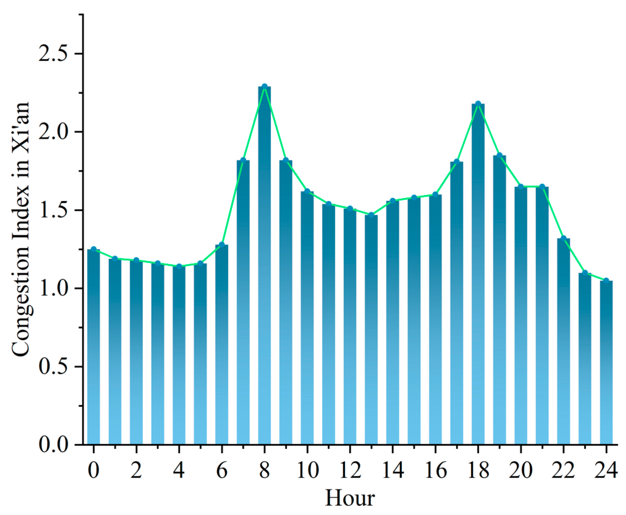
3.3. Data Collection

Traffic volume, as the most important parameter in VISSIM simulation, significantly impacts simulation results in terms of authenticity and accuracy. Compare and evaluate different models by inputting realistic traffic volumes and finally obtain a suitable auxiliary lane design form.

Based on AutoNavi Traffic Big Data’s traffic congestion index statistics for Xi’an in March 2023, the average congestion index for each hour is plotted in Figure 3. It can be seen that traffic in Xi’an City has the highest traffic volume in the morning from 7:00 to 9:00 a.m. and in the afternoon from 17:00 to 19:00 p.m. Therefore, the morning and evening peaks were selected to collect traffic volume data. Good external conditions are a prerequisite for the accuracy of the collected data. Therefore, the data collection was carried out under optimal conditions, ensuring the absence of traffic congestion, road maintenance or construction, good weather conditions, and the absence of traffic accidents. The collection tool was the UAV.

Two UAVs were utilized to collect data simultaneously in the emerging and diverging areas to ensure that traffic volumes on the mainline, emerging, and diverging areas could be captured. The collected data included the following information:

• Traffic volume on the mainline, entrance ramp, and exit ramp;
• The ratio of vehicle types on the mainline and ramps;
• The lane widths of the mainline and ramps and the auxiliary lanes’ length.

As the measurement location is the Xi’an around-city freeway, no buses are operating, only a few intercity coaches. Since the intercity coach count is minimal, and they have a large size and share the same speed limit of 100 km/h as trucks, they are considered trucks in this study. As for minibusses and mid-sized buses, their power characteristics and dimensions are similar to cars; thus, they are categorized as cars. There is no need to differentiate the types of trucks since they all have a speed limit of 100 km/h and are restricted to the outermost lane of the freeway. In the VISSIM software (2022 student), vehicles are classified into three categories: car, truck, and bus. Therefore, this study only focuses on counting the number of trucks and passenger cars.

By processing the collected data, the traffic volume during the morning and evening peak hours was obtained to be 2853 veh/h and 3188 veh/h, respectively. Therefore, the traffic volume in the evening peak hour was selected as the simulation input data (see

Table 4. Traffic volume collection results.

Item	Morning				Evening
Flow	Total	Through	Emerging	Diverging	Total	Through	Emerging	Diverging
Car	2853	1513	526	1340	3188	1548	648	1640
Truck	157	108	57	49	228	184	76	44

) and the collected traffic volume data exhibits the following characteristics:

• Trucks are restricted to the outermost lane due to the mainline lane splitting restriction;
• The proportion of diverging is 51.44%, which is quite large, even larger than the proportion of straight traffic, and the proportion of emerging is 20.33%;
• The proportion of trucks is small, only about 7%.

4. Design Scheme and VISSIM Simulation

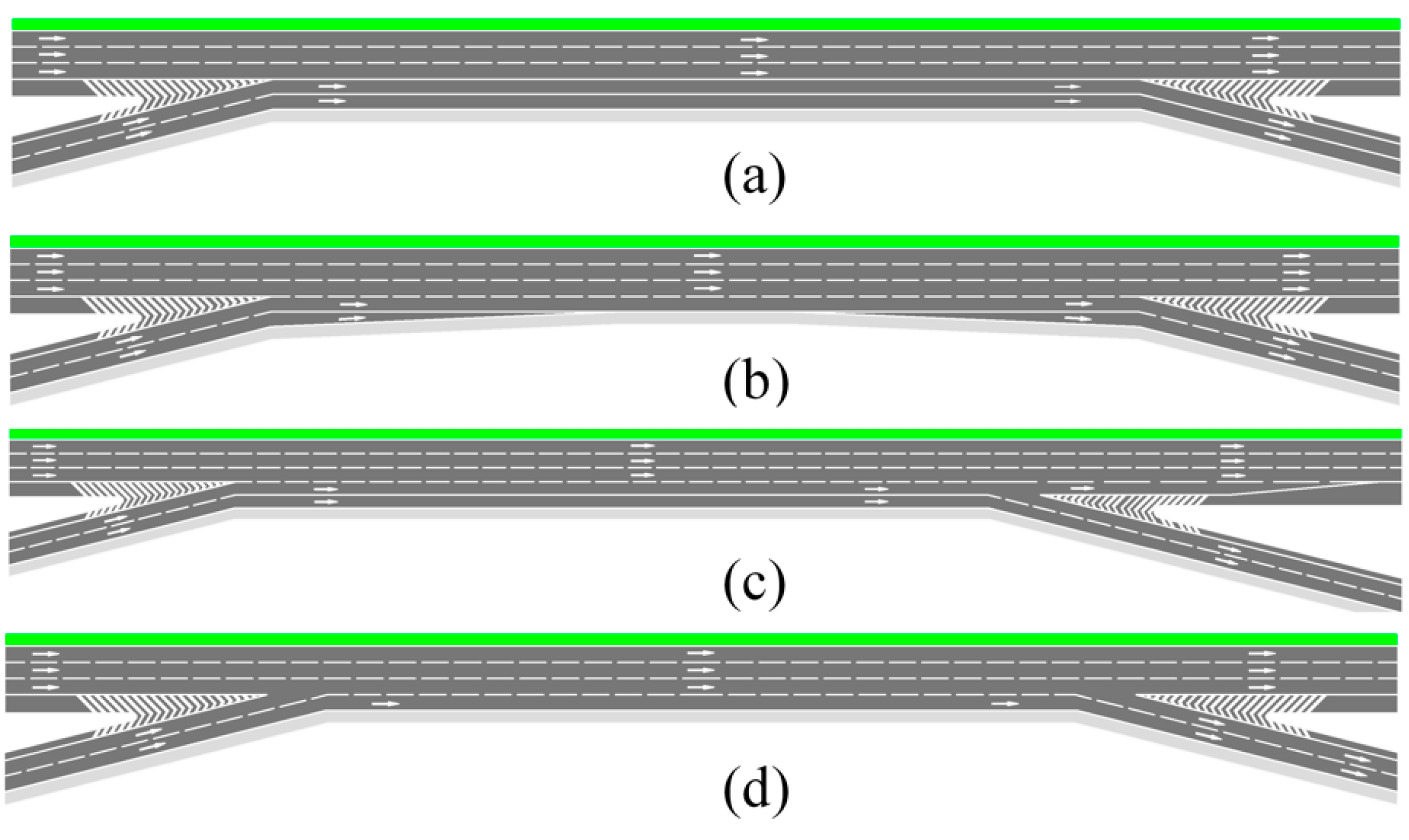
4.1. Design Scheme

For two interchanges spaced evenly apart, the upstream acceleration lanes emerge into the mainline at the taper, the downstream deceleration lanes diverge from the mainline at the taper, and the normal roadway is in between. For small spacing interchange, the traditional connection method will produce weaving in the basic section of the mainline. In particular, for two-lane entrance and exit ramps, the distance between the entrance and exit taper sections is shorter when designed individually, making the use of auxiliary lane connections the most appropriate option. The Baqiao–Tianwang compound interchange uses two auxiliary lanes to connect the upstream acceleration lane and the downstream deceleration lane, called the conventional auxiliary lane connection. Details of the four auxiliary lane design options are as follows.

• Scheme 1: Current Baqiao–Tianwang Interchange Design Scheme

The design is the conventional compound interchange connection method, using auxiliary lanes with the same number of lanes as the ramps to connect the two interchanges, as in Figure 4a. The currently widely adopted design is the conventional auxiliary lane, which is relatively simple. Due to the lack of relevant regulatory guidance, this form of auxiliary lane is typically used for dual-lane entrance and exit ramps. However, when traffic volume is low, the outer auxiliary lane may have a lower utilization rate. Schemes 2–4 differ from Scheme 1 regarding the type of weaving and the utilization of auxiliary lanes. However, Schemes 1–3 are essentially two-lane auxiliary lanes, and Scheme 4 is a single-lane auxiliary lane because it is a B-type weaving.

• Scheme 2: Tapered Auxiliary Lanes

The tapered auxiliary lane is a new design form, as shown in Figure 4b. Based on the conventional auxiliary lane form, the two-lane auxiliary lane tapers to a single lane for a certain distance at the entrance, and then, near the exit, it tapers to two lanes. In this scheme, the auxiliary lane in the basic road section of the mainline is a single lane, which can ensure that the weaving behavior is on the auxiliary lane. However, the auxiliary lane expands to a double-lane configuration near the entrance and exit so as to ensure the efficiency of vehicles diverging and emerging. The use of this design saves land and improves the auxiliary lane utilization ratio.

• Scheme 3: Extend Auxiliary Lanes

According to the “Guidelines for Design of Highway Grade-Separated Intersections” in China, when the traffic volume of the entrance ramp approaches the design capacity, it is specified that the auxiliary lane should be extended at the diverging point, as shown in Figure 4c. This scheme extends the auxiliary lane at the diverging nose for a certain distance and then gradually emerges into the mainline for vehicles that mistakenly enter the auxiliary lane or cannot change lanes in time to emerge into the mainline after entering the auxiliary lane from the acceleration lane. Extending the auxiliary lane beyond the diverging nose ensures sufficient lane length for vehicles to emerge into the mainline and also prevents vehicle parking at the diverging point, which would affect the efficiency and safety of the traffic. However, the “Guidelines” do not specify in detail its application in terms of traffic volume, emerging rate, etc., and there is a lack of guidance in actual design.

• Scheme 4: B-type Weaving Auxiliary Lanes

As shown in Figure 4d, the scheme is to connect the inner lane of the two-lane ramp to the outermost lane of the mainline at the emerging point. Only one auxiliary lane is provided to connect the outer lane of the two-lane ramp. Vehicles located on the inner lane of the ramp can emerge and diverge the mainline without changing lanes.

4.2. Establishing the Model

Currently, traffic simulation represents the most effective method for validating the new design scheme. VISSIM is a microscopic traffic simulation software that efficiently and precisely represents various road design configurations and their operational dynamics. It is commonly used in the evaluation of urban road intersections and the design of interchange entrances and exits [13,45,46]. Therefore, to investigate the impact of different design forms of auxiliary lanes on traffic efficiency and safety, this study uses VISSIM to simulate the four design alternatives in Figure 4.

There are two types of following models in VISSIM, Wiedemannn74 and Wiedemannn99. The former is suitable for urban roads, whereas the latter is mostly used for freeways, so the Wiedemannn99 following model is used in this study [49]. To ensure accurate simulation results, the key parameters in the Wiedemannn99 model were adjusted to align with the Chinese driving behavior characteristics [13,44], and the adjustments are shown in

Table 5. Key driving behavior parameters in Simulation model.

Maximum Deceleration (m/s2)	−1 m/s2 Distance (m)	Acceptable Deceleration (m/s2)	Coordinate Maximum Deceleration of Brakes (m/s2)	Safety Distance Reduction Factor
−4	50	−2	−4	0.5

.

4.3. Calibration of the VISSIM Simulation Model

To ensure the authenticity and accuracy of the simulation model, the model should first be calibrated to minimize the error between the simulation results and the measured data within an acceptable range. The capacity index is highly responsive to the path selection behavior in the model [13], necessitating the utilization of the “capacity calibration method” for model calibration. The mean absolute percentage error (MAPE) reflects the degree of deviation between the simulated value and the measured value. It is commonly used as an evaluation index for the simulation error. The calculation formula for the MAPE is as follows:

$$MAPE=\frac{{\displaystyle \sum _{i=1}^n{C}_v^i-{\displaystyle \sum _{i=1}^n{C}_f^i}}}{{\displaystyle \sum _{i=1}^n{C}_f^i}}$$

(6)

where i denotes the traffic flow, n denotes the total number of traffic flows, $C_v^i$ denotes the simulated capacity in VISSIM (veh/h), and $C_f^i$ denotes the measured capacity (veh/h).

According to relevant studies, a simulation model is generally considered accurate in simulating the actual traffic situation when the MAPE value is less than 15% [50,51].

The MAPE calculation results are presented in

Table 6. VISSIM simulation calibration results.

Flow	Through Traffic	Diverging Traffic	Emerging Traffic
Investigated capacity (veh/h)	1732	1684	724
Simulated capacity (veh/h)	1576.8	1620	648
Individual MAPE (%)	−8.96%	−3.8%	−10.5%
MAPE (%)	0.28%

. Based on the data in Table 6, the error is 0.28%, which is less than 15%, indicating that the accuracy of the simulation model meets the requirements.

4.4. Operational Efficiency and Environmental Assessment

4.4.1. Selection of Evaluation Indexes

The evaluation of different schemes using VISSIM is based on several indexes, including delays, travel time, and number of stops, common indexes for evaluating operational efficiency [52]. Under normal driving conditions, freeways do not generate congestion, so the queue length is not meaningful for freeways. In addition, CO emissions and fuel consumption were selected for evaluating the environmental impact.

4.4.2. Analysis of Simulation Results

The four auxiliary lane design forms proposed in Section 4 helped establish VISSIM models and input of the measured traffic parameters. Therefore, the indexes of each model in terms of traffic efficiency and environment can be obtained (see

Table 7. Simulation results for transportation efficiency and environmental indexes.

Item	Scheme 1	Scheme 2	Scheme 3	Scheme 4
Travel time (s)	77.81	84.2	70.96	74.86
Delay (s)	2.58	4.73	1.30	1.44
Number of stops	0.036	0.10	0.009	0.007
CO emissions (g)	5967.36	5350.25	4948.78	5019.775
Fuel consumption (gallon)	85.39	76.54	70.78	71.78

).

Upon examining the simulation results in Table 7, it is apparent that Scheme 2 exhibits comparatively unfavorable outcomes regarding travel time, delay, and number of stops compared to the other three schemes under the measured traffic volume. This indicates that Scheme 2 has the lowest traffic efficiency under the measured traffic volume. This situation occurs because the auxiliary lanes of Scheme 2 are tapered from two to one, and the vehicles on the outer auxiliary lanes need to change lanes centrally, reducing traffic efficiency.

On the remaining efficiency indexes, Scheme 3 performs best, with varying degrees of improvement in all aspects. Notably, Scheme 3 exhibits the most significant improvement in delays, with a decrease of 49.6%. This improvement in delays is the most notable among all the indexes measured. Scheme 4 has a slightly lower efficiency improvement than Scheme 3.

In terms of CO emissions, the improvement effect of Schemes 3 and 4 increased by 7.53% and 6.22%, respectively, compared with Scheme 1. Schemes 3 and 4 have high traffic efficiency and stable vehicle speed, greatly reducing fuel consumption and controlling pollutant emissions.

4.5. Safety Evaluation

4.5.1. Selection of Evaluation Indexes

In addition to the analysis of the above indexes, the design should be evaluated from the perspective of safety, and the safety of the design schemes can be reflected in the collision frequency. Therefore, the SSAM(X86) software proposed by the Federal Highway Administration (FHWA) was used to evaluate the safety performance of the freeway. By inputting the trajectory data file obtained from the VISSIM simulation into the SSAM(X86) software, the probability of conflict can be predicted, and three indexes can be generated. These indexes include time to collision (TTC), post-encroachment time (PET), and number of conflicts, all of which help characterize safety aspects.

In the SSAM(X86) software, the minimum TTC is set to 1.5 s, and less than 1.5 s is considered to have the possibility of a conflict. PET refers to the duration between the leading vehicle leaving a designated area and the following vehicle arriving at the same location. A traffic conflict is considered to occur when the PET is less than 5 s [53]. TTC and PET can better predict the propensity of collision.

However, due to the high speed of vehicles, the freeway diverging and emerging areas often produce serious consequences once a collision occurs. Therefore, using the CSI index to evaluate the collision’s severity is also necessary. TTC and Max-delta V are collision-related indexes, and based on their relationship, the CSI index can be calculated as shown in (7) [54].

$$CSI=e^{-TTC}\left(\frac{1}{TTC+\frac{a}{MaxDeltaV}}\right)$$

(7)

where Max-Delta V is the vehicle speed change of pre-crash, which can be output via the SSAM(X86) software, and the a is a constant to balance the contribution of the TTC and Max-Delta V to severity, which is taken as a = 20.

In addition, based on the angle between two conflicting vehicles, conflicts can be categorized into rear-end conflicts, lane change conflicts, and crossing conflicts. The total number of the various conflicts is the number of conflicts [48].

Among the selected indexes mentioned above, TTC and PET are positive indexes, while CSI and the number of conflicts are negative indexes.

4.5.2. Analysis of Simulation Results

In addition to evaluating the traffic efficiency and environment of the design scheme, safety is also an important factor that directly affects the safety of the driver’s life and property. Traffic accidents in real situations can seriously affect traffic efficiency, so it is important to evaluate the schemes from a safety perspective. Trajectory files of each scheme were imported into SSAM for safety analysis, and the results are shown in

Table 8. Safety analysis results.

Scheme	Rear end	Lane Change	Crossing	TTC	PET	CSI
1	32	30	0	0.36	0.35	0.24
2	22	16	0	0.23	0.31	0.17
3	15	33	0	0.24	0.32	0.20
4	173	10	0	0.15	0.03	0.27

.

As can be seen from Table 8, Scheme 2, despite having the lowest traffic efficiency, exhibits better security with the fewest number of conflicts and the smallest CSI. The safety indexes of Scheme 4 are worse than the other schemes, and the security is the worst. Compared with Scheme 1, Scheme 3 has a certain degree of improvement in security. There are no crossing conflicts due to the small angle at which the traffic flows in the straight, diverging, and emerging directions.

Collision frequency and severity were predicted by TTC, PET, and CSI indexes. When TTC and PET are large, it means that the driver has more time to adjust to avoid collisions. The results show that the collision frequency of the four schemes is Schemes 4, 1, 3, and 2 in descending order. In terms of collision severity, Scheme 2 has the lowest severity, followed by Scheme 3, while the collision between Schemes 1 and 4 is serious.

In summary, it can be seen that the two new designs, Schemes 2 and 3, offer a good improvement in safety.

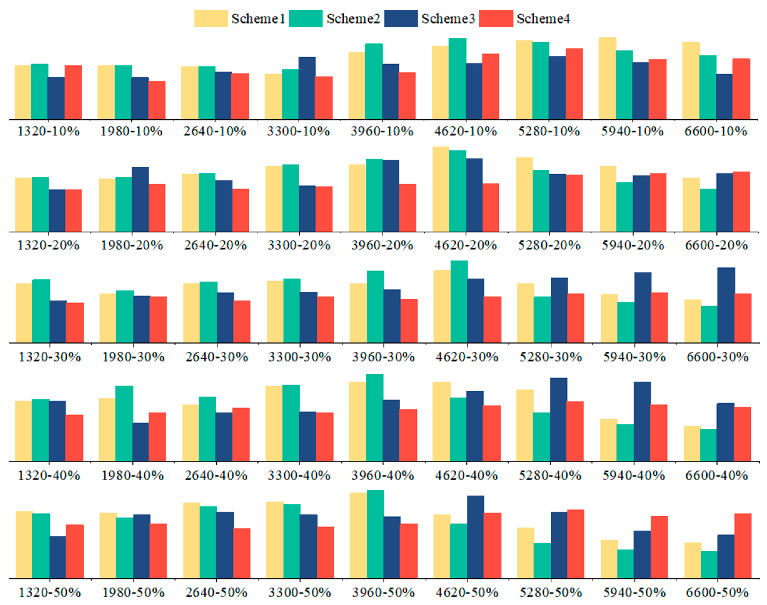
5. Sensitivity Analysis

5.1. Sensitivity Factors Determination

Through the above comparison of the four schemes, Scheme 3 is optimal in terms of traffic efficiency and environmental protection, and Scheme 2 is optimal regarding safety. However, the conclusions are based on measured data and are limited to a particular traffic volume and diverging and emerging ratios. It cannot reflect the advantages and disadvantages of the schemes for other traffic volume conditions, and the conclusions lack universality.

Therefore, for the proposed different schemes to be reasonably applied in compound interchanges, it is necessary to use VISSIM to simulate various traffic conditions and obtain conclusive results.

According to the service traffic volume of the basic section of freeway stipulated in China’s “Technical Standards of Highway Engineering” [55], the traffic volume of a three-lane freeway is 2250 veh/h when the service level is grade I, 6600 veh/h when the service level is grade VI, and the measured traffic volume is 3758 veh/h. Therefore, the traffic volume range considered is from 0.2 to 1.0 V/C during the sensitivity analysis, and the traffic volume under the condition of 1.0 V/C is 6600 veh/h. Typically, the number of diverging vehicles is less than that of vehicles traveling straight through, but the measured diverging ratio is 51.44%. Therefore, the diverging and emerging 10–50% ratio was taken for sensitivity analysis. The traffic volume and diverging–emerging ratio combinations are listed in

Table 9. Sensitivity analysis results on traffic volume.

Item	Value
Traffic volume (veh/h)	1320/1980/2640/3300/3960/4620/5280/5940/6600
Diverging and emerging ratio (%)	10/20/30/40/50

for a total of 45 traffic combinations.

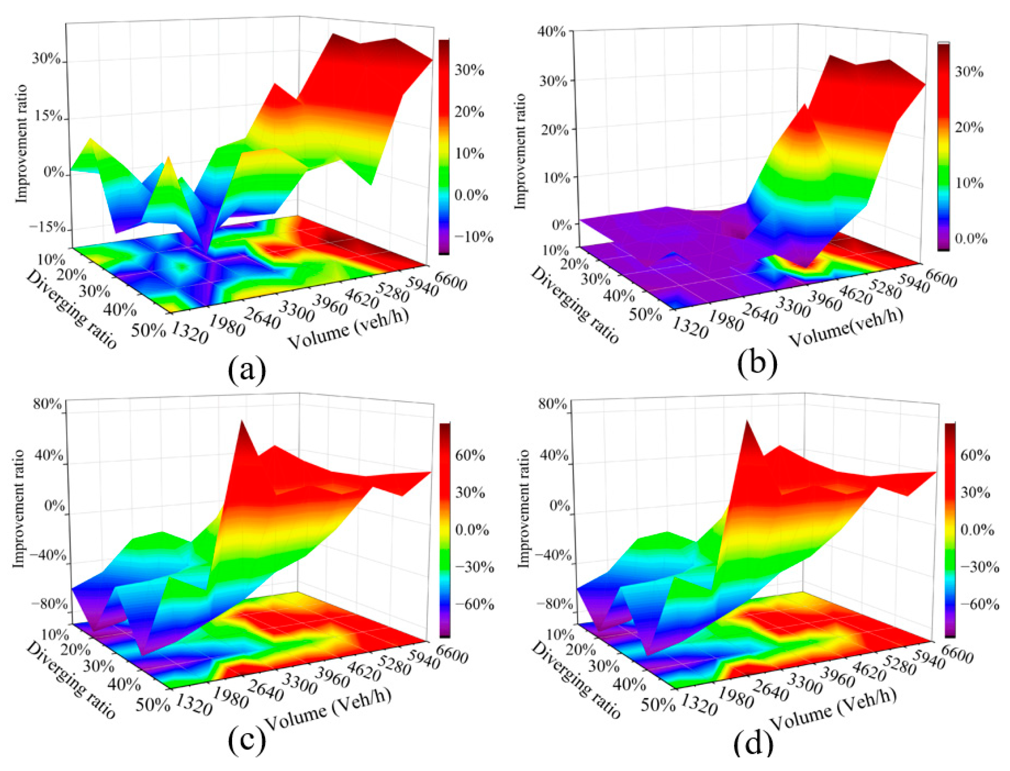
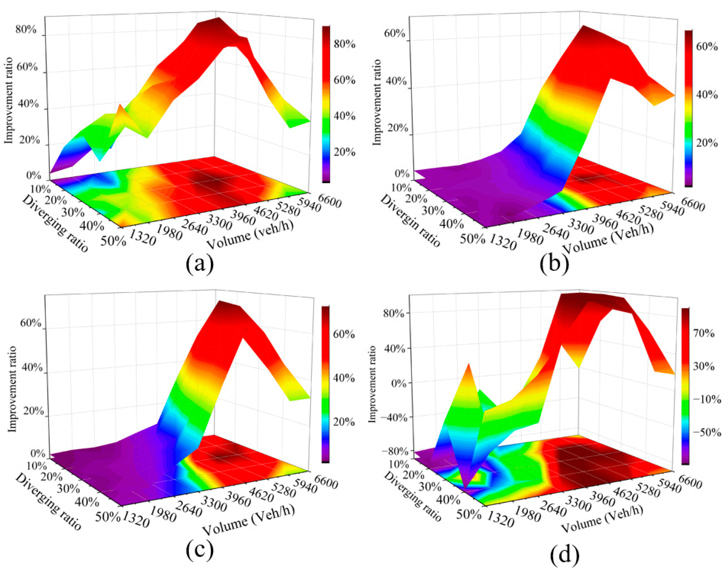
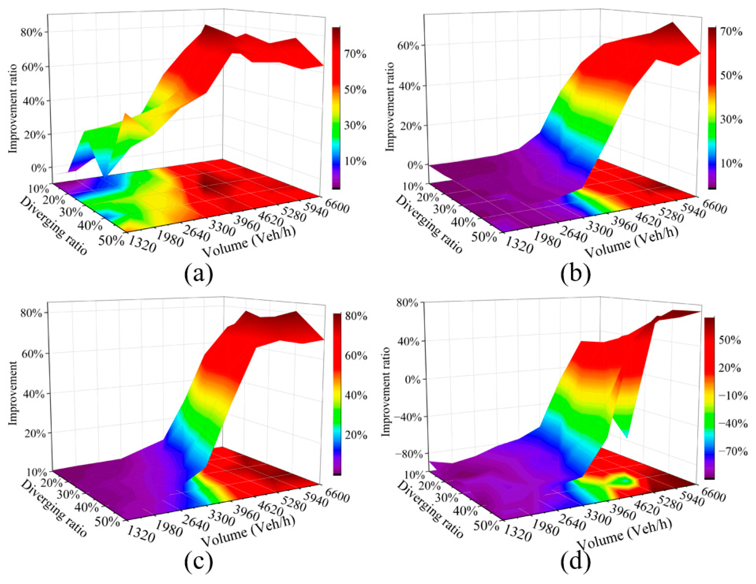
5.2. Sensitivity Analysis Results

In the sensitivity analysis, some indexes do not change significantly or have the same trend of change, so this section selects representative indexes for comparison. In terms of traffic efficiency, the number of stops value is very small, even 0 when the traffic volume is small; in terms of environmental indexes, CO and fuel consumption have the same trend; and in terms of safety, the comparison of the number of conflicts between the schemes is the most significant.

Therefore, four indexes, delay, travel time, CO emissions, and number of conflicts, were chosen to perform a comparative analysis of the schemes.

• Comparison of Scheme 2 and Scheme 1

Using Scheme 1 as the comparator, we calculated the improvement ratio of the four indexes in Scheme 2 relative to Scheme 1 and plotted the improvement ratio in Figure 5.

From Figure 5a, it can be seen that there is no significant change in delay between Scheme 2 and Scheme 1 for several traffic volumes at the diverging ratio of 10%. However, as the diverging ratio and traffic volume increased, the delays of Scheme 2 improved significantly, with a maximum improvement of 37.13% when the traffic volume exceeded 4620 veh/h and the diverging ratio surpassed 10%.

The design purpose of the auxiliary lane is to reduce the impact on straight traffic. Therefore, Figure 5b represents the travel time in the straight direction. It can be seen from Figure 5 that Scheme 2 has varying degrees of improvement in travel times under various traffic combinations. The most significant improvement was observed when the diverging ratio exceeded 20%, and the traffic volume was greater than 4620 veh/h.

Figure 5c shows the improvement in CO emissions of Scheme 2. It is evident that Scheme 2 exhibits lower CO emissions compared to Scheme 1 under all traffic combinations. Additionally, the improvement ratio shows a positive correlation with increasing traffic volumes.

Figure 5d shows a negative improvement in the number of conflicts for Scheme 2 compared to Scheme 1 at the diverging ratio of 10%. However, as the diverging ratio increased, the negative improvement in the number of conflicts in Scheme 2 decreased with the increase in traffic volume, eventually transforming into a positive improvement.

There is no notable disparity in traffic efficiency between Schemes 1 and 2 when the traffic volume remains below 4620 veh/h. Both schemes can effectively accommodate the freeway’s capacity at this lower traffic volume range. When the traffic volume is low, the number of conflicts is small for both schemes. It is at higher traffic volumes that a significant difference in the number of conflicts became apparent between the two schemes. Therefore, although there is a negative improvement in the number of conflicts for Scheme 2 at low traffic levels, overall, Scheme 2 is better than Scheme 1 in terms of safety. In summary, Scheme 2 is superior to Scheme 1 regarding efficiency, safety, and environmental protection.

• Comparison of Scheme 3 and Scheme 1

From Figure 6a, it is evident that Scheme 3 significantly reduces delays across all traffic conditions. The improvement ratio reaches the maximum at 30%, 5280 veh/h, and the maximum value is 89.62%. After that, the improvement ratio decreases as the traffic volume and diverging ratio increase.

Based on Figure 6b, it can be seen that Scheme 3 has a positive improvement in travel time in all cases. However, the improvement ratio is small within the traffic volume of 1320–3960 veh/h. Remarkably, the improvement ratio increases rapidly when the traffic volume exceeds 3960 veh/h and reaches a maximum of 66.45% at 30%, 5280 veh/h.

Figure 6c shows that Scheme 3 demonstrates a substantial improvement in CO emissions compared to Scheme 1. There is no notable distinction between Scheme 3 and Scheme 1 for all diverging ratios within the traffic volume range of 1320 to 3300 veh/h, only a small improvement in CO emissions. The improvement ratio of Scheme 3 exhibits its greatest significance when the traffic volume surpasses 3300 veh/h.

Figure 6d shows that at the diverging ratio of 10–40% and traffic volumes of 1320–3960 veh/h, Scheme 1 has a much lower number of conflicts and higher safety. However, when the traffic volume exceeds 3960 veh/h, Scheme 3 has a greater improvement ratio in the number of conflicts, reaching a maximum of 100%. When the diverging ratio is 50%, the improvement is positive for all traffic volumes.

This situation occurs due to the escalating traffic volumes and diverging ratio; the demand for diverging and emerging increases, resulting in complex traffic conditions upstream of the diverging area. For Scheme 1, vehicles in the auxiliary lanes have no insertion gap to emerge into the mainline. As a result, they need to slow down or even stop, leading to waiting near the diverging area. This situation contributes to an increase in the number of conflicts. However, Scheme 2 extends the auxiliary lane to a certain distance behind the diverging nose to ensure that vehicles have enough distance to emerge into the mainline.

From the above analysis, it can be seen that Scheme 3 outperforms Scheme 1 in terms of efficiency, environmental protection, and safety. This difference becomes particularly pronounced when the diverging ratio exceeds 30% and the traffic volume exceeds 3960 veh/h. In these scenarios, the improvement is most obvious.

• Comparison of Scheme 4 and Scheme 1

Figure 7a shows that Scheme 4 has a higher delay than Scheme 1 when the diverging ratio of 10% and traffic volume range from 1320 to 1680 veh/h. However, for the rest of the traffic combinations, there is a significant improvement, typically within the range of 30% to 75%. The maximum improvement, reaching 84.69%, is achieved at 30%, 4620 veh/h.

Figure 7b shows that Scheme 4 demonstrates either no improvement or minimal improvement in terms of travel time when the traffic volume remains below 4620 veh/h. The improvement ratio is greater when the traffic volume is greater than 4620 veh/h. The maximum improvement ratio reaches 71.67% at 40%, 6600 veh/h.

Figure 7c shows that Scheme 4 improves CO emissions under all traffic conditions, and the improvement becomes larger as the diverging ratio increases but gradually decreases when the diverging ratio exceeds 40%. The maximum improvement ratio occurs at 40%, 6600 veh/h.

In terms of the number of conflicts, Scheme 4 presents a disadvantage, with no improvement in the diverging ratio of 10%. For the rest of the diverging ratio cases, when the traffic volume is only 5280–6600 veh/h, there is a large improvement ratio in Scheme 4.

In summary, since Scheme 4 is the B-type weaving area, some vehicles directly emerge into the mainline without changing lanes, so the traffic efficiency is high. However, it is important to note that Scheme 4 has certain inherent drawbacks. Specifically, the absence of auxiliary lanes for transitioning on the emerging ramp, which directly emerges into the mainline, poses a significant risk for accidents. Therefore, it verifies the situation in Figure 7d; the safety is poorer compared to Scheme 1.

6. Comprehensive Analysis Based on the FAEWM

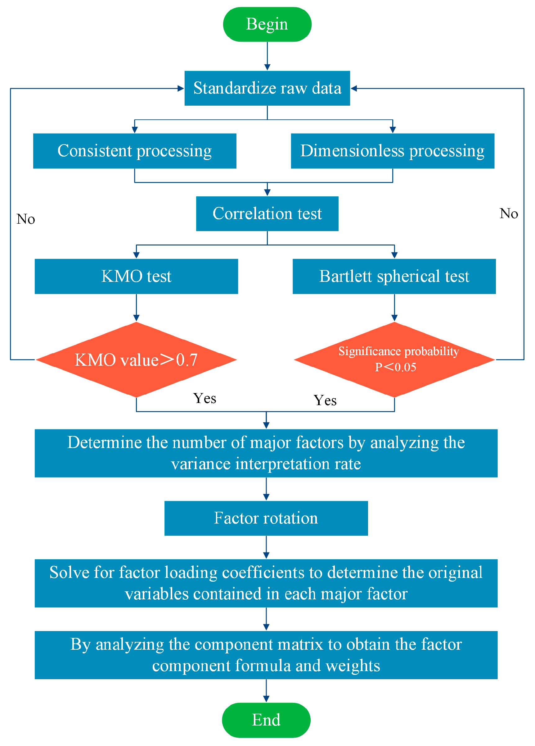
6.1. Determination of Weights Based on the Factor Analysis Method

In the sensitivity analysis, nine indexes were chosen to evaluate the different schemes, and this particular index was excluded because the value of the number of stops was too small. In order to streamline the evaluation indexes and facilitate the evaluation of the schemes, the FAM was used to simplify the remaining eight indexes.

Using the FAM is a process of downscaling high-dimensional data. The original variables are linearly combined into principal ingredients by studying the internal dependencies between the original variables. To minimize the loss of information on the original variables, multiple indexes are transformed into several comprehensive indexes independent of each other. This allows the comprehensive indexes to reflect the vast majority of the information of the original variables. The flowchart of the FAM is shown in Figure 8.

The detailed steps of the factor analysis method are outlined below.

Xi denotes the eight indexes obtained from the simulation results, i is the serial number of the indexes, and p is the number of traffic condition grouping (refer to (8)).

$$X={\left[X_1,X_2,\cdots ,X_i\right]}^T$$

(8)

where X_i can be represented as:

$$\left[\begin{array}{c}{X}_1\\ X_2\\ ⋮\\ X_i\end{array}\right]=\left[\begin{array}{cccc}{\alpha }_{11}& {\alpha }_{12}& \cdots & {\alpha }_{1p}\\ {\alpha }_{21}& {\alpha }_{22}& \cdots & {\alpha }_{2p}\\ ⋮& ⋮& \cdots & ⋮\\ {\alpha }_{i1}& {\alpha }_{i2}& \cdots & {\alpha }_{ip}\end{array}\right]\left[\begin{array}{c}{F}_1\\ F_2\\ ⋮\\ F_p\end{array}\right]+\left[\begin{array}{c}{\epsilon }_1\\ {\epsilon }_2\\ ⋮\\ {\epsilon }_i\end{array}\right]$$

(9)

where the coefficient matrix ${\alpha }_{ip}$ is the factor loadings, $A=({\alpha }_{ip})$ is the factor loading matrix, F is the common factor, and $\epsilon$ is the special factor.

Step 1: Standardization of the Raw Data

• Consistent processing

The eight selected indexes encompass various characteristics, with larger values indicating preferable scheme performance for positive indexes while smaller values indicate better performance for inverse indexes. To maintain consistency among the indexes, all are transformed into positive indexes, normalized using (10).

$${x^{\prime }}_{ip}=\max \left\{x_i\right\}-x_{ip}$$

(10)

• Dimensionless processing

As different indexes have different dimensions, the difference in magnitude of the values can be very large, which may result in indexes with smaller magnitudes being ignored. Therefore, it is necessary to eliminate the dimensions of all indexes. The linear normalization method is used for processing, and the specific calculation formula is shown in (11).

$${x^{″}}_{ip}=\frac{{x^{\prime }}_{ip}-\min \left\{x_{ip}{}^{\prime }\right\}}{\max \left\{x_{ip}{}^{\prime }\right\}-\min \left\{x_{ip}{}^{\prime }\right\}}(i=1\mathrm{to}10; p=1\mathrm{to}45)$$

(11)

where ${\tilde{x}}_{ip}$ denotes the standardized index, $\min \left\{x_{ip}{}^{\prime }\right\}$ denotes the minimum value of the index, and $\max \left\{x_{ip}{}^{\prime }\right\}$ denotes the maximum value of the index.

Step 2: Correlation test

Before conducting factor analysis, it is necessary to conduct the KMO and Bartlett’s sphericity tests to determine whether the original variables are strongly correlated or not. If the correlation is weak, factor analysis may not be suitable or informative for the given variables.

• KMO test

The KMO value is within [0, 1], where a higher value indicates a stronger correlation among the variables. A KMO value above 0.7 is generally considered suitable for factor analysis, implying that the variables are sufficiently interrelated to proceed with the analysis.

• Bartlett’s test of sphericity

Bartlett’s test of sphericity is used to assess the interdependence among variables. If the test reveals that the variables are independent of each other, it implies that factor analysis cannot be performed. When the p-value is less than 0.05, it suggests that there is a correlation between the variables, and factor analysis can be performed.

Step 3: Solve for Factor Loadings

The principal ingredient analysis (PCA) is used to determine the factor loadings. In the PCA, the eigenvalue decomposition of the covariance matrix is performed to obtain the eigenvalues and eigenvectors of the correlation coefficient matrix R. The eigenvalues and eigenvectors are denoted as (12) and (13), respectively.

$$\lambda =\left[{\lambda }_1,{\lambda }_2,\cdots ,{\lambda }_i\right]$$

(12)

$$U=\left[u_1,u_{2,}\cdots ,u_i\right]$$

(13)

Then, the loading matrix A of the principal ingredient analysis for the correlation coefficient matrix R is calculated using (14).

$$A=\left(\sqrt{{\lambda }_1}{u}_1,\sqrt{{\lambda }_2}{u}_2,\cdots ,\sqrt{{\lambda }_i}{u}_i\right)$$

(14)

Step 4: Factor Rotation

The loading matrix obtained from the principal ingredient analysis solution in Step 3 is not unique. The original variables may have exhibited high loadings on the different common factors before factor rotation, leading to an inability to interpret the meaning of the common factors. The values in the loading matrix undergo appropriate factor transformation to polarize them, resulting in newly transformed factors that exhibit a more distinct difference.

Step 5: Calculate Factor Scores

To evaluate the different schemes, it is necessary to obtain the values of the principal ingredients. Therefore, it is necessary to calculate the scores of each original variable on the principal ingredients. The estimates of the principal ingredient scores can be calculated via the parameter estimation method.

Using KMO and Bartlett’s test of sphericity to examine the correlation among the original variables in the four schemes to determine whether FAM could be used, the test results are shown in

Table 10. Results of KMO and Bartlett’s test of sphericity.

		Scheme 1	Scheme 2	Scheme 3	Scheme 4
KMO test	Value	0.754	0.769	0.863	0.798
Bartlett’s test of sphericity	Approximate chi-square	1554	2111	1983	1399
	Degree of freedom	28	28	28	28
	Significance	0	0	0	0

.

As can be seen in Table 10, the probability of significance of all four schemes is 0, and the KMO value is greater than 0.7, indicating that the data satisfy the suitability criteria for the FAM.

Table 11. Variance interpretation table (Scheme 1).

Total Variance Explained
Ingredient	Explanatory Rate of Variance before Rotation			Explanatory Rate of Variance after Rotation
	Characteristic Root	Explanation of Variance (%)	Cumulative Variance Explained (%)	Characteristic Root	Explanation of Variance (%)	Cumulative Variance Explained (%)
1	5.605	70.064	70.064	475.613	59.452	59.452
2	1.516	18.95	89.013	203.629	25.454	84.905
3	0.766	9.572	98.585	109.441	13.68	98.585
4	0.045	0.566	99.152
5	0.041	0.512	99.664
6	0.023	0.292	99.956
7	0.003	0.044	100
8			100

,

Table 12. Variance interpretation table (Scheme 2).

Total Variance Explained
Ingredient	Explanatory Rate of Variance before Rotation			Explanatory Rate of Variance after Rotation
	Characteristic Root	Explanation of Variance (%)	Cumulative Variance Explained (%)	Characteristic Root	Explanation of Variance (%)	Cumulative Variance Explained (%)
1	5.353	66.906	66.906	495.513	61.939	61.939
2	1.763	22.042	88.948	183.463	22.933	84.872
3	0.758	9.479	98.427	108.442	13.555	98.427
4	0.099	1.242	99.669
5	0.014	0.175	99.844
6	0.01	0.131	99.975
7	0.002	0.025	100
8			100

,

Table 13. Variance interpretation table (Scheme 3).

Total Variance Explained
Ingredient	Explanatory Rate of Variance before Rotation			Explanatory Rate of Variance after Rotation
	Characteristic Root	Explanation of Variance (%)	Cumulative Variance Explained (%)	Characteristic Root	Explanation of Variance (%)	Cumulative Variance Explained (%)
1	5.806	72.57	72.57	490.35	61.294	61.294
2	1.221	15.265	87.836	183.231	22.904	84.198
3	0.785	9.808	97.644	107.569	13.446	97.644
4	0.14	1.756	99.4
5	0.022	0.28	99.68
6	0.018	0.221	99.901
7	0.008	0.099	100
8			100

and

Table 14. Variance interpretation table (Scheme 4).

Total Variance Explained
Ingredient	Explanatory Rate of Variance before Rotation			Explanatory Rate of Variance after Rotation
	Characteristic Root	Explanation of Variance (%)	Cumulative Variance Explained (%)	Characteristic Root	Explanation of Variance (%)	Cumulative Variance Explained (%)
1	6.631	82.891	82.891	419.801	52.475	52.475
2	0.96	11.996	94.887	204.234	25.529	78.004
3	0.183	2.293	97.18	153.407	19.176	97.18
4	0.101	1.257	98.437
5	0.081	1.014	99.451
6	0.032	0.396	99.847
7	0.012	0.153	100
8			100

show the total variance explained tables of the four schemes, which indicate the contribution of the factors to the explanation of the variables, i.e., all the variables can be explained using several common factors.

The higher the variance explained rate, the greater the importance of the principal ingredient and the higher the weight assigned to that ingredient. Typically, ingredients with a pre-rotation eigenroot greater than 1 are selected as principal ingredients while ensuring the cumulative variance explained rate is greater than 80%. Three ingredients are needed to express more than 95% of the information content of all variables in Table 11, Table 12, Table 13 and Table 14, so three common factors are extracted.

After identifying the three common factors, it is necessary to specify the importance of each original variable in each common factor. This is performed by calculating the factor loading coefficients, as shown in

Table 15. Factor loading coefficients after rotation (Scheme 1).

Original Variable	Rotated Factor Loading Coefficients			Commonality
	Factor 1	Factor 2	Factor 3
Delay	0.968	0.163	−0.167	0.992
Travel time	0.958	0.19	−0.171	0.983
CO emission	0.947	0.254	−0.173	0.992
Fuel consumption	0.947	0.254	−0.173	0.992
TTC	0.14	0.978	0.072	0.981
PET	0.298	0.933	−0.14	0.979
CSI	−0.272	−0.022	0.962	0.999
Number of conflicts	0.96	0.134	−0.169	0.968

,

Table 16. Factor loading coefficients after rotation (Scheme 2).

Original Variable	Rotated Factor Loading Coefficients			Commonality
	Factor 1	Factor 2	Factor 3
Delay	0.981	0.09	−0.157	0.995
Travel time	0.974	0.122	−0.167	0.992
CO emission	0.978	0.142	−0.139	0.997
Fuel consumption	0.978	0.142	−0.139	0.997
TTC	−0.04	0.96	0.177	0.955
PET	0.317	0.916	−0.092	0.949
CSI	−0.246	0.089	0.964	0.998
Number of conflicts	0.983	0.046	−0.155	0.992

,

Table 17. Factor loading coefficients after rotation (Scheme 3).

Original Variable	Rotated Factor Loading Coefficients			Commonality
	Factor 1	Factor 2	Factor 3
Delay	0.968	0.152	−0.173	0.989
Travel time	0.963	0.184	−0.157	0.985
CO emission	0.942	0.297	−0.135	0.995
Fuel consumption	0.942	0.297	−0.135	0.995
TTC	0.126	0.968	0.021	0.954
PET	0.535	0.787	−0.083	0.912
CSI	−0.213	−0.009	0.977	1.000
Number of conflicts	0.958	0.207	−0.149	0.982

and

Table 18. Factor loading coefficients after rotation (Scheme 4).

Original Variable	Rotated Factor loading Coefficients			Commonality
	Factor 1	Factor 2	Factor 3
Delay	0.872	0.459	0.079	0.977
Travel time	0.921	0.34	0.13	0.981
CO emission	0.778	0.505	0.329	0.968
Fuel consumption	0.778	0.505	0.329	0.968
TTC	0.124	0.98	0.1	0.986
PET	0.389	0.717	0.519	0.935
CSI	−0.248	−0.115	0.937	0.975
Number of conflicts	0.735	0.654	0.12	0.983

.

As can be seen from Table 15, Table 16, Table 17 and Table 18, TTC and PET have the highest loading coefficients on Factor 2. Since TTC and PET are evaluation indexes for accident frequency prediction, Factor 2 can be categorized as the “accident frequency prediction factor”. CSI has the largest loading factor on Factor 3, referred to as the “accident severity factor”. Similarly, the rest of the variables load more heavily on Factor 1, named the “efficiency–environment factor”, as these indexes evaluate the efficiency and the environment.

Table 19. Ingredient matrix.

Item		Delay	Travel Time	Number of Conflicts	TTC	PET	CSI	CO Emission	Fuel Consumption
Scheme 1	Ingredient 1	0.243	0.233	0.245	−0.116	−0.117	0.196	0.217	0.217
	Ingredient 2	−0.074	−0.055	−0.09	0.568	0.521	−0.01	−0.014	−0.014
	Ingredient 3	0.076	0.067	0.073	0.079	−0.127	1.075	0.059	0.059
Scheme 2	Ingredient 1	0.218	0.209	0.224	−0.086	−0.054	0.181	−1.198	1.628
	Ingredient 2	−0.044	−0.023	−0.072	0.558	0.531	−0.079	0.244	−0.275
	Ingredient 3	0.062	0.043	0.073	0.036	−0.179	1.065	−0.066	0.815
Scheme 3	Ingredient 1	0.248	0.242	0.236	−0.219	−0.054	0.177	0.479	−0.061
	Ingredient 2	−0.133	−0.109	−0.09	0.719	0.474	−0.035	0.321	−0.355
	Ingredient 3	0.035	0.049	0.055	−0.029	−0.029	1.06	0.188	−0.07
Scheme 4	Ingredient 1	0.522	0.892	0.571	−0.239	−0.295	0.546	0.173	0.173
	Ingredient 2	−0.384	−0.162	0.188	0.891	0.333	−0.034	−0.014	−0.014
	Ingredient 3	−0.19	−0.139	−0.137	−0.049	−0.274	1.095	0.063	0.063

shows the factor score included in each principal ingredient.

Based on the score of each original variable in Table 19, the score calculation formula for each principal ingredient is shown in (15). The calculated weights of the principal ingredients are included in

Table 20. Factor weighting results.

	Principal Ingredient 1	Principal Ingredient 2	Principal Ingredient 3
Scheme 1	60.305%	25.819%	13.876%
Scheme 2	62.929%	23.299%	13.772%
Scheme 3	62.773%	23.457%	13.771%
Scheme 4	53.998%	26.27%	19.732%

.

$$\{\begin{array}{l}{F}_1=a_1{x}_1+a_2{x}_2+\cdots +a_8{x}_8\\ F_2{=\mathrm{b}}_1{x}_1+b_2{x}_2+\cdots +b_8{x}_8\\ F_3{=\mathrm{c}}_1{x}_1+c_2{x}_2+\cdots +c_8{x}_8\end{array}$$

(15)

where F₁, F₂, and F₃ denote the main ingredient s; a_i, b_i, and c_i denote the score coefficients of each original variable in the main ingredients; and x_i denotes the value of the original variable after standardization.

In summary, by using factor analysis, the eight original variables selected were downscaled to three common factors, F₁, F₂, and F₃, with F₁ being the “efficiency–environment factor”, F₂ being the “accident frequency prediction factor”, and F₃ being the “accident severity factor”.

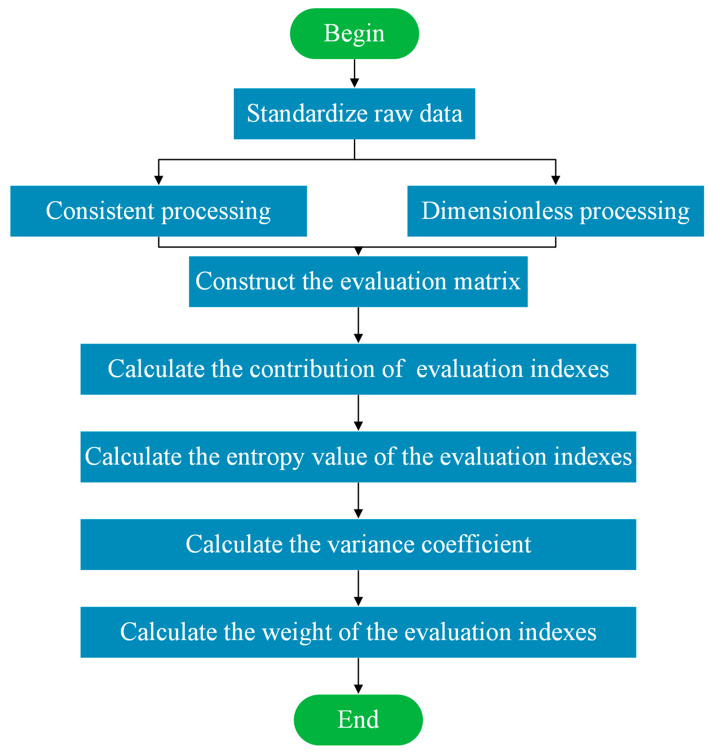
6.2. Determination of Factor Weights Based on the Entropy Method

The entropy value can be utilized to assess the degree of dispersion of a specific index. A smaller information entropy value indicates a higher degree of dispersion for the index, resulting in a greater weight assigned to the index in the overall evaluation. Employing information entropy to calculate each index’s weight provides a foundation for the comprehensive evaluation of multiple indexes. The flowchart of the EWM is shown in Figure 9.

The detailed calculation steps are as follows.

Step 1: Construct the evaluation matrix.

The results of the eight indexes of the four schemes under 45 traffic conditions were formed into a matrix, as shown in (16).

$$X_o=\left[D_{op},T_{op},E_{op},F_{op},C_{op},TT{C}_{op},PE{T}_{op},CS{I}_{op}\right]$$

(16)

where o denotes the design schemes number; p denotes the combination of traffic conditions, p = 1 to 45; D denotes delay; T denotes travel time; E denotes CO emissions; F denotes fuel consumption; and C denotes the number of conflicts.

The simulation results of Scheme 1 are represented as a matrix of 8 columns and 45 rows (refer to (17)).

$$X_1=\left[D_{1\mathrm{p}},T_{1p},E_{1p},F_{1p},C_{1p},TT{C}_{1\mathrm{p}},PE{T}_{1p},CS{I}_{1p}\right]$$

(17)

Among

$$D_{1p}={\left[D_{1,1},D_{1,2},\cdots ,D_{1,45}\right]}^T$$

(18)

In order to evaluate the results of the evaluation indexes of the four schemes under the same traffic combinations, the matrix of the four schemes was decomposed and reorganized to obtain the matrix A_S, shown in (19).

$$A_s=\left[\begin{array}{l}{X}_1(s,\cdot )\\ X_2(s,\cdot )\\ X_3(s,\cdot )\\ X_4(s,\cdot )\end{array}\right]$$

(19)

where $X_1\left(s,\cdot \right)$ denotes the sth row of X₁, i.e., the results of the eight indexes under the sth traffic combination.

Denote each element in matrix A_S by y_pq to obtain the new matrix Y (refer to (20)).

$$Y=\left[\begin{array}{cccc}{y}_{11}& y_{12}& \cdots & y_{1q}\\ y_{21}& y_{22}& \cdots & y_{2q}\\ ⋮& ⋮& ⋮& ⋮\\ y_{p1}& y_{p2}& \cdots & y_{pq}\end{array}\right]$$

(20)

where p denotes the number of schemes, p = 1 to 4, and q denotes the number of indexes, q = 1 to 8.

Step 2: Calculate the contribution of the qth evaluation index in the pth program.

$$p_{pq}=\frac{y_{pq}}{{\displaystyle \sum _p^n{y}_{pq}}}$$

(21)

Step 3: Calculate the entropy value of the qth evaluation index.

$$e_q=-\frac{1}{\ln \left(n\right)}{\displaystyle \sum _p^n{p}_{pq}\ln \left(p_{pq}\right)}$$

(22)

Step 4: Calculate the coefficient of variation.

$$d_q=1-e_q$$

(23)

Step 5: Calculate the weight of each evaluation index.

$$w_q=\frac{d_q}{{\displaystyle \sum _q^n{d}_q}}$$

(24)

The results of calculating the weights of each factor via the EWM are shown in

Table 21. Factor weighting results based on the EWM (%).

	Item	Scheme 1	Scheme 2	Scheme 3	Scheme 4
Factor 1	Delay	7.133	8.821	5.832	4.863
	Travel time	8.451	9.924	7.133	4.859
	CO emission	9.903	10.593	7.890	8.054
	Fuel consumption	9.903	10.593	7.890	8.054
	Number of conflicts	10.235	10.736	6.380	13.708
Factor 2	TTC	18.332	14.222	21.226	8.257
	PET	25.595	28.376	34.777	34.068
Factor 3	CSI	10.449	6.734	8.871	18.136

.

6.3. Determination of Evaluation Index Weights

The EWM determines the weight of each index based on its degree of variation, which is an objective empowerment method and not affected by subjective factors. However, it can not reduce the dimensionality of the evaluation indexes. The FAM is subjective in determining the principal ingredients by specifying criteria such as an eigenvalue greater than 1 or a cumulative contribution exceeding 80%. Considering the shortcomings of a single evaluation model, this paper adopts two methods, the FAM and the EWM, to calculate the weights of evaluation indexes by combining the advantages of the two methods to make the assignment more accurate. The comprehensive weight value of each principal ingredient is shown in

Table 22. Principal ingredient weight values (%).

	Principal Ingredient	Principal Ingredient Entropy Weights	Principal Ingredient Variance Contribution Ratio	Combined Weight
Scheme 1	F1	45.625	60.305	52.97
	F2	43.927	25.819	34.87
	F3	10.449	13.876	12.16
Scheme 2	F1	50.668	62.929	56.80
	F2	42.598	23.299	32.95
	F3	6.734	13.772	10.25
Scheme 3	F1	35.126	62.773	48.95
	F2	56.003	23.457	39.73
	F3	8.871	13.771	11.32
Scheme 4	F1	39.539	53.998	46.77
	F2	42.325	26.27	34.30
	F3	18.136	19.732	18.93

.

In summary, the compound interchange auxiliary lane design form is quantitatively scored by (25).

$$S=w_1{F}_1{}^{\prime }+w_2{F}_2{}^{\prime }+w_3{F}_3{}^{\prime }$$

(25)

where w is the value of the combination weights and $F^{\prime }$ is the score of the original variable on the principal ingredients.

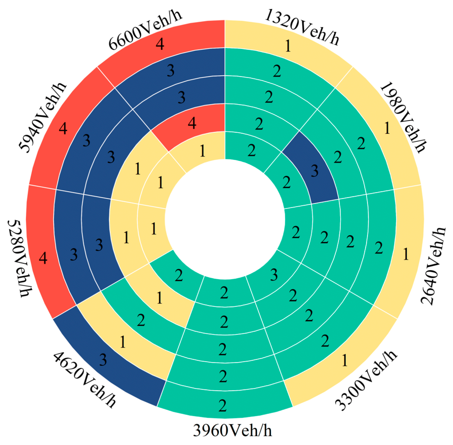
7. Results and Discussion

7.1. Discussion of the Calculations Results

We used (25) to calculate the scores of the four schemes under different traffic conditions; the scores are plotted in Figure 10. The best scheme under each traffic combination was also selected and plotted in Figure 11.

As can be seen in Figure 10 and Figure 11, Scheme 1 has the highest scores under traffic volumes of 5280–6600 veh/h and a diverging ratio of 10–20%, or traffic volumes of 1320–3300 veh/h and diverging ratio of 50%. This suggests that Scheme 1 should be used primarily when traffic volumes are high and the diverging ratio is low or where traffic volumes are low and the diverging ratio is high. The two-lane auxiliary lane can accommodate more vehicles when the traffic volume or diverging–emerging ratio is large. Meanwhile, Figure 10 shows that Scheme 1 scores second only to Scheme 2, and the gap between the two is small, so Scheme 1 has better applicability.

Scheme 2 utilizes a unique design form that tapers the two-lane auxiliary lane to a single lane. It scored the highest at low traffic volumes of 1320–3960 veh/h and a diverging ratio of 10–40%. On the one hand, the design ensures that vehicles can efficiently enter or exit the mainline under a larger diverging–emerging ratio. This improvement enhances the capacity of the freeway while preserving the advantages of two lanes at the entrance and exit. On the other hand, once the vehicle enters the mainline of the freeway if the traffic volume is low, the vehicle can quickly change lanes to the mainline. Therefore, the auxiliary lanes exhibit a low utilization rate of the outer lane, and the single-lane auxiliary lanes can ensure the vehicle’s diverging and emerging needs. This indicates that the design of Scheme 2 adapts well to small traffic volumes. However, as the traffic volume and diverging–emerging ratio increase, the score of Scheme 2 decreases significantly and is smaller than the remaining three schemes.

Scheme 3 achieves its highest score with large traffic volumes and a significant diverging–emerging ratio. For example, traffic volumes ranging from 5280 to 6600 veh/h and a diverging–emerging ratio of 30–40%. Due to the heavy traffic volume on both the mainline and auxiliary lanes, vehicles on the auxiliary lanes cannot change lanes to the mainline. However, Scheme 3 extends the inner auxiliary lane to a certain distance behind the diverging nose. This design allows vehicles to continue moving and change lanes to the mainline after passing through the heavily congested diverging area. Thus, Scheme 3 performs better in high-traffic conditions.

The score of Scheme 4 is highest only for the extreme case where the traffic volume and diverging ratio are the highest, but this is rarely the case in practice. Although the design of Scheme 4 makes it possible for vehicles to emerge into the mainline without changing lanes, it also brings some safety problems, resulting in a low comprehensive score. Therefore, Scheme 4 is less applicable.

In summary, the traffic volume and diverging–emerging ratio greatly impact the choice of auxiliary lane form. Scheme 2 has the best improvement effect in the case of both low traffic volume and diverging–emerging ratio, and Scheme 3 has better performance in the case of both high traffic volume and diverging–emerging ratio. The conclusions obtained via the FAEWM provide a reliable basis for engineering design and maximize traffic efficiency and safety while simultaneously mitigating environmental pollution. For the design of compound interchange auxiliary lanes, the design form can be selected directly based on the traffic volume and the diverging–emerging ratio. However, the scheme selected in Figure 11 under various traffic combinations is based on a comprehensive score, and there may still be a disadvantage in one of the evaluation indexes.

For example, a reasonable selection of auxiliary lane design forms can effectively improve pollutant emissions. Through the comparison of four solutions, it can be observed that as traffic volume increases, both Scheme 2–4 show significant improvements in CO emissions, particularly Scheme 3 and Scheme 4, with the highest improvement rate reaching 80%. Notably, while Solution 4 performs relatively poorly in terms of safety and efficiency, it exhibits substantial environmental improvement.

However, selecting design solutions needs to consider multiple aspects and should not solely prioritize environmental protection at the expense of efficiency and safety improvements. In reality, as long as traffic efficiency is enhanced and traffic congestion is alleviated, it can reduce vehicle exhaust emissions.

7.2. Discussion of Computational Modeling Applications

When evaluating multiple models or cases and dealing with multiple evaluation indexes, assessing the merits of different options through a single index becomes challenging. In such situations, it is necessary to consider multiple indexes comprehensively and normalize them for comparison. Particularly when there are numerous evaluation indexes, the method proposed in this paper can simplify the data and provide more meaningful interpretations. The FAEWM is suitable for the following situations: when there are a large number of evaluation indexes or dimensions, when there are complex relationships among the data, and when there is a high correlation between the evaluation indexes.

However, when there are few evaluation indexes, the data do not meet the basic assumptions of the FAM, or there is no correlation among the evaluation indexes, the FAEWM cannot be used.

The FAEWM can be implemented in practical applications through the following steps:

Firstly, the FAM can be used to uncover common factors or latent structures among variables, reducing the complexity of the data. By employing the FAM, original variables can be transformed into fewer and more meaningful factors, aiding in understanding the structure and patterns of the data.

Next, the EWM can be utilized to determine the weights of factors or criteria and evaluate their relative superiority or inferiority. The EWM calculates weights based on the information entropy of the criteria, considering the importance and distinctiveness of different factors or criteria. This allows for quantifying their relative significance in decision-making or evaluation processes.

7.3. Validation of the FAEWM

In order to verify the validity and reliability of the FAEWM, we use the simulation results obtained from the measured traffic volume data. As shown in the Data Collection section, the traffic volume is 3188 veh/h, and the diverging ratio is 51.44%. The simulation results of the four schemes with measured traffic data are listed in

Table 23. Simulation results with measured traffic volume.

	The Number of Conflicts	TTC	PET	CSI	Travel Time	Delay	CO Emissions	Fuel Consumption
1	62	0.36	0.35	0.24	77.81	2.58	5967.36	85.39
2	38	0.23	0.31	0.17	84.2	4.73	5350.25	76.54
3	48	0.24	0.32	0.20	70.96	1.3	4948.78	70.78
4	183	0.15	0.03	0.27	74.86	1.44	5019.78	71.78

.

From Table 23, it can be seen that Scheme 1 is the best in terms of TTC and PET, Scheme 2 is the best in terms of number of conflicts and CSI, Scheme 3 is the best in terms of travel time, delays, fuel consumption, and CO emissions, while Scheme 4 performs average in all aspects. It can be seen that Scheme 3 performs better in terms of traffic efficiency, while Schemes 1 and 2 perform better in terms of safety.

Based on the scores obtained for each solution under different traffic configurations (Figure 10), it can be observed that Schemes 1 and 2 have similar scores under measured traffic conditions. However, as the traffic volume continues to increase, the score for Scheme 3 gradually improves and surpasses Schemes 1 and 2. It is evident that around the measured traffic volume, the difference in traffic efficiency between Scheme 1 and Scheme 2 is not significant compared to Scheme 3, but there is a significant safety improvement. Therefore, when the traffic volume is relatively low, Schemes 1 and 2 receive higher scores. However, as the traffic volume exceeds the maximum capacity of Schemes 1 and 2, the improvement in traffic efficiency for Scheme 3 leads to an increase in its score, making it the optimal solution.

In summary, the results obtained using the FAEWM are consistent with the actual situation and verify the reliability of the FAEWM method.

8. Conclusions

The rapid construction of freeways, especially the expansion of the around-city freeway, inevitably produces more and more compound interchanges. The complex weaving behavior of compound interchanges seriously impacts traffic efficiency and safety. However, compound interchanges in China have various auxiliary lane forms, and the lack of specific standards for selecting the appropriate forms has led to some design problems regarding efficiency, safety, and land utilization.

In this study, four auxiliary lane design forms were proposed for compound interchanges, which were simulated via VISSIM traffic simulation software based on measured data. To comprehensively assess the reliability of the four schemes in terms of traffic efficiency, safety, and environmental protection, several evaluation indexes were selected, using the FAM to downsize the indexes and combine them with the EWM for comprehensive weighting to accurately, intuitively, and efficiently select the appropriate design scheme. The proposed auxiliary lane form can be widely used in small spacing interchanges under different traffic conditions and transformed into a compound interchange. This implementation aimed to enhance traffic efficiency, improve driving safety, and promote environmental protection capability. The conclusions obtained in this study can be summarized as follows.

• The auxiliary lanes of Scheme 1 were most effective under specific traffic conditions. When the traffic volume was less than 3960 veh/h, the diverging–emerging ratio was higher than 40%; when the traffic volume exceeded 3960 veh/h, the diverging-emerging ratio was 10–20%. However, in practice, the score gap between Schemes 1 and 2 is so small that they can be substituted for each other at low traffic volumes and low diverging–emerging ratios;
• Scheme 2 had the most advantages under low traffic volume and diverging–emerging ratio. Specifically, when the traffic volume is below 3960 veh/h and the diverging–emerging ratio is 10–40%, opting for Scheme 2 as the auxiliary lane form is recommended. This scheme proved to be adaptable and suitable for a wide range of traffic situations. In addition, its unique design can save much land and has good adaptability in terrain-restricted areas;
• When the traffic volume surpasses 3960 veh/h, and the diverging–emerging ratio exceeds 20%, it is advisable to select Scheme 3 as the preferred auxiliary lane form;
• The Scheme 4 B-type weaving area has the worst safety. This design leads to the inner ramp vehicles emerging directly into the mainline, interfering with straight vehicles and generating many conflicts. The more vehicles in the inner lanes of the ramp, the more serious the interference;
• The environmental impact of different types of auxiliary lanes varies greatly, up to 81.05%. A reasonable choice of auxiliary lane form is conducive to improving the environment.

The proposed design forms for continuous auxiliary lanes in this article demonstrate good applicability. They can be applied to newly constructed and existing freeways to ensure economic efficiency and space-saving.

For existing compound interchanges, when the conventional continuous auxiliary lanes fail to meet the current traffic capacity, they can be reconfigured according to Scheme 3, which involves extending the auxiliary lanes at the diverging nose. When the design meets the traffic capacity requirements and considers the slight difference between conventional auxiliary lanes and taper auxiliary lanes, the original form of conventional auxiliary lanes can be maintained.

For newly constructed compound interchanges, the above-mentioned findings can be referred to.

Limited to space, only a one-way, three-lane freeway was studied in this paper. Due to the fast growth rate of traffic volume in recent years, it is anticipated that future expansion projects will result in the development of an increased number of four-lane or even five-lane freeways. As a consequence, the following issues need to be considered. Firstly, further research is conducted for the case of different numbers of the mainline lanes. Secondly, focus must be placed on whether the interchange spacing affects the form of auxiliary lanes. Finally, the applicability of the recommended auxiliary lanes form proposed in this study on three-lane ramps should be considered. The authors intend to prioritize these issues in future studies.

References

1. MunOz, J.C.; Daganzo, C.F. The bottleneck mechanism of a freeway diverge. Transp. Res. Part A Policy Pract. 2002, 36, 483–505. [Google Scholar] [CrossRef]
2. Sarhan, M.; Hassan, Y.; Halim, A.O.A.E. Safety performance of freeway sections and relation to length of speed-change lanes. Rev. Can. Génie Civ. 2008, 35, 531–541. [Google Scholar] [CrossRef]
3. Wang, Z.; Chen, H.; Lu, J.J. Exploring Impacts of Factors Contributing to Injury Severity at Freeway Diverge Areas. Transp. Res. Rec. 2018, 2102, 43–52. [Google Scholar] [CrossRef]
4. Ali, Y.; Zheng, Z.D.; Haque, M.M.; Yildirimoglu, M.; Washington, S. CLACD: A complete Lane-Changing decision modeling framework for the connected and traditional environments. Transp. Res. Part C-Emerg. Technol. 2021, 128, 103162. [Google Scholar] [CrossRef]
5. Fatema, T.; Ismail, K.; Hassan, Y. Validation of Probabilistic Model for Design of Freeway Entrance Speed Change Lanes. Transp. Res. Rec. 2014, 2460, 97–106. [Google Scholar] [CrossRef]
6. Wang, R.H.; Hu, J.B.; Zhang, X.Q. Analysis of the Driver’s Behavior Characteristics in Low Volume Freeway Interchange. Math. Probl. Eng. 2016, 2016, 2679516. [Google Scholar] [CrossRef]
7. Chen, D.W.; Cheng, S.W.; Liu, J.Y.; Zhang, J.; You, X.Y. A Simulation-Based Optimization Method for Truck-Prohibit Ramp Placement along Freeways. Math. Probl. Eng. 2023, 2023, 4170669. [Google Scholar] [CrossRef]
8. Ahammed Mohammad, A.; Hassan, Y.; Sayed Tarek, A. Modeling Driver Behavior and Safety on Freeway Merging Areas. J. Transp. Eng. 2008, 134, 370–377. [Google Scholar] [CrossRef]
9. McCartt, A.T.; Northrup, V.S.; Retting, R.A. Types and characteristics of ramp-related motor vehicle crashes on urban interstate roadways in Northern Virginia. J. Saf. Res. 2004, 35, 107–114. [Google Scholar] [CrossRef]
10. Zhang, X.; Wang, J.B.; Li, T.N.; Sun, J. Safety factors of exit slip roads on China’s urban motorways. Proc. Inst. Civ. Eng. Transp. 2017, 170, 276–286. [Google Scholar] [CrossRef]
11. Chen, W.; Li, H.; Hou, E.K.; Wang, S.Q.; Wang, G.R.; Panahi, M.; Li, T.; Peng, T.; Guo, C.; Niu, C.; et al. GIS-based groundwater potential analysis using novel ensemble weights-of-evidence with logistic regression and functional tree models. Sci. Total Environ. 2018, 634, 853–867. [Google Scholar] [CrossRef] [PubMed]
12. Persson, P.O. A sparse and high-order accurate line-based discontinuous Galerkin method for unstructured meshes. J. Comput. Phys. 2013, 233, 414–429. [Google Scholar] [CrossRef]
13. Pan, B.H.; Xie, Z.J.; Liu, S.R.; Shao, Y.; Cai, J.J. Evaluating Designs of a Three-Lane Exit Ramp Based on the Entropy Method. IEEE Access 2021, 9, 53436–53451. [Google Scholar] [CrossRef]
14. Ledesma, R.D.; Ferrando, P.J.; Trogolo, M.A.; Poo, F.M.; Tosi, J.D.; Castro, C. Exploratory factor analysis in transportation research: Current practices and recommendations. Transp. Res. Part F-Traffic Psychol. Behav. 2021, 78, 340–352. [Google Scholar] [CrossRef]
15. Zhang, K.R.; Hassan, M.; Yahaya, M.; Yang, S.P. Analysis of Work-Zone Crashes Using the Ordered Probit Model with Factor Analysis in Egypt. J. Adv. Transp. 2018, 2018, 8570207. [Google Scholar] [CrossRef]
16. Zhang, C.; He, J.; Wang, Y.H.; Yan, X.T.; Zhang, C.J.; Chen, Y.K.; Liu, Z.Y.; Zhou, B.J. A Crash Severity Prediction Method Based on Improved Neural Network and Factor Analysis. Discret. Dyn. Nat. Soc. 2020, 2020, 4013185. [Google Scholar] [CrossRef]
17. Kong, X.Q.; Das, S.; Zhou, H.M.; Zhang, Y.L. Characterizing phone usage while driving: Safety impact from road and operational perspectives using factor analysis. Accid. Anal. Prev. 2021, 152, 106012. [Google Scholar] [CrossRef]
18. Liu, P.; Chen, H.Y.; Lu, J.J.; Cao, B. How Lane Arrangements on Freeway Mainlines and Ramps Affect Safety of Freeways with Closely Spaced Entrance and Exit Ramps. J. Transp. Eng. 2010, 136, 614–622. [Google Scholar] [CrossRef]
19. Huang, L.H.; Zhao, X.H.; Li, Y.; Ma, J.M.; Yang, L.P.; Rong, J.; Wang, Y. Optimal design alternatives of advance guide signs of closely spaced exit ramps on urban expressways. Accid. Anal. Prev. 2020, 138, 105465. [Google Scholar] [CrossRef]
20. Li, Z.B.; Wang, W.; Liu, P.; Bai, L.; Du, M.Q. Analysis of Crash Risks by Collision Type at Freeway Diverge Area Using Multivariate Modeling Technique. J. Transp. Eng. 2015, 141, 04015002. [Google Scholar] [CrossRef]
21. Liao, Y.G.; Yang, Y.; Ding, Z.Z.; Tong, K.M.; Zeng, Y.J. Risk Distribution Characteristics and Optimization of Short Weaving Area for Complex Municipal Interchanges. J. Adv. Transp. 2021, 2021, 5573335. [Google Scholar] [CrossRef]
22. Kusuma, A.; Liu, R.H.; Choudhury, C.; Montgomery, F. Analysis of the Driving Behaviour at Weaving Section Using Multiple Traffic Surveillance Data. In Proceedings of the 17th Meeting of the EURO-Working-Group on Transportation (EWGT), Seville, Spain, 2–4 July 2014; pp. 51–59. [Google Scholar]
23. Kwon, E.; Lau, R.; Aswegan, J. Maximum possible weaving volume for effective operations of ramp-weave areas—Online estimation. In Proceedings of the 79th Annual Meeting of the Transportation-Research-Board, Washington, DC, USA, 9–13 January 2000; pp. 132–141. [Google Scholar]
24. Al-Jameel, H. Characteristics of the driver behaviour in weaving sections: Empirical study. Int. J. Eng. Technol. Res. 2017, 2, 1430–1446. [Google Scholar]
25. Skabardonis, A. Simulation of freeway weaving areas. In Proceedings of the 81st Annual Meeting of the Transportation-Research-Board, Washington, DC, USA, 13–17 January 2002; pp. 115–124. [Google Scholar]
26. Mai, T.; Jiang, R.; Chung, E. A Cooperative Intelligent Transport Systems (C-ITS)-based lane-changing advisory for weaving sections. J. Adv. Transp. 2016, 50, 752–768. [Google Scholar] [CrossRef]
27. Shang, T.; Lian, G.; Zhao, Y.C.; Liu, X.L.; Wang, W.J. Off-Ramp Vehicle Mandatory Lane-Changing Duration in Small Spacing Section of Tunnel-Interchange Section Based on Survival Analysis. J. Adv. Transp. 2022, 2022, 9427052. [Google Scholar] [CrossRef]
28. Le, T.Q.; Porter, R.J. Safety Evaluation of Geometric Design Criteria for Spacing of Entrance-Exit Ramp Sequence and Use of Auxiliary Lanes. Transp. Res. Rec. 2012, 2309, 12–20. [Google Scholar] [CrossRef]
29. Guo, Y.Q. Effects of Ramp Spacing on Freeway Mainline Crashes. In Proceedings of the ICCET 2011, Jinan, China, 14–16 October 2011; pp. 95–99. [Google Scholar]
30. Park, B.J.; Fitzpatrick, K.; Lord, D. Evaluating the Effects of Freeway Design Elements on Safety. Transp. Res. Rec. 2010, 2195, 58–69. [Google Scholar] [CrossRef]
31. Fitzpatrick, K.; Porter, R.J.; Pesti, G.; Chu, C.L.; Park, E.S.; Le, T. Guidelines for Spacing Between Freeway Ramps. Transp. Res. Rec. 2011, 2262, 3–12. [Google Scholar] [CrossRef]
32. Liu, Y.T.; Pan, B.H.; Zhang, Z.L.; Zhang, R.Y.; Shao, Y. Evaluation of Design Method for Highway Adjacent Tunnel and Exit Connection Section Length Based on Entropy Method. Entropy 2022, 24, 1794. [Google Scholar] [CrossRef]
33. Chen, S.K.; Mao, B.H.; Liu, S.; Sun, Q.X.; Wei, W.; Zhan, L.X. Computer-aided analysis and evaluation on ramp spacing along urban expressways. Transp. Res. Part C-Emerg. Technol. 2013, 36, 381–393. [Google Scholar] [CrossRef]
34. Chen, D.W.; Mo, F.X.; Chen, Y.; Zhang, J.; You, X.Y. Optimization of Ramp Locations along Freeways: A Dynamic Programming Approach. Sustainability 2022, 14, 9718. [Google Scholar] [CrossRef]
35. Ma, J.; Zeng, Y.L.; Chen, D.W. Ramp Spacing Evaluation of Expressway Based on Entropy-Weighted TOPSIS Estimation Method. Systems 2023, 11, 139. [Google Scholar] [CrossRef]
36. Zhang, G.; Sun, D.H.; Zhao, M. Phase transition of a new lattice hydrodynamic model with consideration of on-ramp and off-ramp. Commun. Nonlinear Sci. Numer. Simul. 2018, 54, 347–355. [Google Scholar] [CrossRef]
37. Zhao, J.Y.; Guo, Y.Y.; Liu, P. Safety impacts of geometric design on freeway segments with closely spaced entrance and exit ramps. Accid. Anal. Prev. 2021, 163, 106461. [Google Scholar] [CrossRef]
38. Huang, Z.F.; Zhang, Z.H.; Li, H.J.; Qin, L.Q.; Rong, J. Determining Appropriate Lane-Changing Spacing for Off-Ramp Areas of Urban Expressways. Sustainability 2019, 11, 2087. [Google Scholar] [CrossRef]
39. Sato, H.; Xing, J.; Tanaka, S.; Morikita, K. Examining the Effect of Connecting Auxiliary Lanes on Mitigation of Expressway Traffic Congestion. Int. J. Intell. Transp. Syst. Res. 2011, 9, 55–63. [Google Scholar] [CrossRef]
40. Shea, M.S.; Le, T.Q.; Porter, R.J. Combined Crash Frequency-Crash Severity Evaluation of Geometric Design Decisions Entrance-Exit Ramp Spacing and Auxiliary Lane Presence. Transp. Res. Rec. 2015, 2521, 54–63. [Google Scholar] [CrossRef]
41. Qi, Y.; Wang, Y.B.; Chen, X.S.; Cheu, R.L.; Yu, L.; Teng, H.L. Methods of dropping auxiliary lanes at freeway weaving segments. Transp. Plan. Technol. 2018, 41, 389–401. [Google Scholar] [CrossRef]
42. Wang, X.F.; Ding, Z.Z.; Guo, K.; Lin, Y.J. A Simulation-Based Comprehensive Analysis for Traffic Efficiency and Spatial Distribution of Risks in Short Weaving Area of Municipal Interchange. J. Adv. Transp. 2021, 2021, 9968426. [Google Scholar] [CrossRef]
43. Wang, Y.P.; Xu, J.; Liu, X.L.; Zheng, Z.J.; Zhang, H.S.; Wang, C.Y. Analysis on Risk Characteristics of Traffic Accidents in Small-Spacing Expressway Interchange. Int. J. Environ. Res. Public Health 2022, 19, 9938. [Google Scholar] [CrossRef]
44. Liu, X.J.; Shao, C.Y.; Yang, S.; Zhang, R.Y.; Pan, B.H. Study on the location of unconventional outside left-turn lane at signalized intersections based on an entropy method. Front. Environ. Sci. 2022, 10, 970836. [Google Scholar] [CrossRef]
45. Pan, B.H.; Chai, H.; Liu, J.; Shao, Y.; Liu, S.R.; Zhang, R.Y. Evaluating Operational Features of Multilane Turbo Roundabouts with an Entropy Method. J. Transp. Eng. Part A-Syst. 2022, 148, 04022072. [Google Scholar] [CrossRef]
46. Pan, B.H.; Liu, S.R.; Xie, Z.J.; Shao, Y.; Li, X.; Ge, R.C. Evaluating Operational Features of Three Unconventional Intersections under Heavy Traffic Based on CRITIC Method. Sustainability 2021, 13, 4098. [Google Scholar] [CrossRef]
47. AASHTO. A Policy on Geometric Design of Highways and Streets; AASHTO: Washington, DC, USA, 2018. [Google Scholar]
48. Roadway Design Section. Guidelines for Design of Highway Grade-Separated Intersections; JTG/T D21; Arizona Department of Transportation: Phoenix, AZ, USA, 2014.
49. PTV. PTV Vissim 2022 User Manual; PTV China: Shanghai, China, 2022. [Google Scholar]
50. Xiang, Y.; Li, Z.B.; Wang, W.; Chen, J.X.; Wang, H.; Li, Y. Evaluating the Operational Features of an Unconventional Dual-Bay U-Turn Design for Intersections. PLoS ONE 2016, 11, e0158914. [Google Scholar] [CrossRef] [PubMed]
51. Sun, J. Guideline for Microscopic Traffic Simulation Analysis; Tongji University Press: Shanghai, China, 2014. [Google Scholar]
52. Henclewood, D.; Suh, W.; Rodgers, M.O.; Fujimoto, R.; Hunter, M.P. A calibration procedure for increasing the accuracy of microscopic traffic simulation models. Simul.-Trans. Soc. Model. Simul. Int. 2017, 93, 35–47. [Google Scholar] [CrossRef]
53. Lili, P.; Rahul, J. Surrogate Safety Assessment Model (SSAM)-Software User Manual; Federal Highway Administration: Washiton, DC, USA, 2008.
54. Liu, Q.J.; Deng, J.L.; Shen, Y.F.; Wang, W.X.; Zhang, Z.; Lu, L.J. Safety and Efficiency Analysis of Turbo Roundabout with Simulations Based on the Lujiazui Roundabout in Shanghai. Sustainability 2020, 12, 7479. [Google Scholar] [CrossRef]
55. JTG B01-2014; Technical Standard of Highway Engineering. Ministry of Transport of PRC: Bejing, China, 2014.
Figure 1. Distribution of interchanges on the Xi’an around-city freeway.
Applsci 13 10499 g001
Figure 2. Baqiao–Tianwang compound interchange.
Applsci 13 10499 g002
Figure 3. Traffic congestion index map of Xi’an.
Applsci 13 10499 g003
Figure 4. Design form scheme of the auxiliary lane. (a) Conventional auxiliary lane design; (b) tapered auxiliary lane design; (c) extended auxiliary lane design; (d) B-type weaving auxiliary lane design.
Applsci 13 10499 g004
Figure 5. Improvement ratio of Scheme 2 compared to Scheme 1. (a) Delay, (b) travel time, (c) CO emission, and (d) number of conflicts.
Applsci 13 10499 g005
Figure 6. Improvement ratio of Scheme 3 compared to Scheme 1. (a) Delay, (b) travel time, (c) CO emission, and (d) number of conflicts.
Applsci 13 10499 g006
Figure 7. Improvement ratio of Scheme 4 compared to Scheme 1. (a) Delay, (b) travel time, (c) CO emission, and (d) number of conflicts.
Applsci 13 10499 g007
Figure 8. Flowchart of the FAM.
Applsci 13 10499 g008
Figure 9. Flowchart of the EWM.
Applsci 13 10499 g009
Figure 10. Auxiliary lane design schemes score.
Applsci 13 10499 g010
Figure 11. Optimal solutions under different traffic combinations (numbers 1–4 in the figure denote the optimal solutions under different traffic combinations; the circle has five layers, representing the diverging ratio of 10%, 20%, 30%, 40%, and 50% from the inside to the outside; the same radial direction denotes the same traffic volume).
Applsci 13 10499 g011