3. Numerical Modeling of Double-Pulse Anti-Stokes Order
The theory describing MRG by A.P. Hickman et al. is based on a multi-wave approach where all the Raman orders are mutually coupled together in the process [
16]. The Raman orders including the two pumps form a set of frequency components
, where
is the pump frequency and
is the Raman frequency. The resonant Raman process is described by the interaction of the fields using the two-photon Bloch equations [
16,
17], and the authors obtained the following equations describing a generalized Rabi frequency
:
with on-resonance Rabi frequency
and total detuning
given by:
where the
are the amplitudes of the j-th Raman order,
is the complex conjugate of
,
are the transition moments, I is the total intensity of all orders, and
is the detuning between the frequency separation of the pumps and the Raman frequency. As can be seen from Equation (3), the detuning
is determined by three terms, the Raman frequency detuning
, the time derivative of the Rabi phase
, and the two-photon Stark shift due to the coupling of the polarizabilities,
, and total pulse intensity. The Hickman theory assumed steady state pumps. Rickes et al. showed adiabatic population transfer by a time-varying, two-photon laser-induced Rabi frequency shift [
17]. The time-dependent two-photon Bloch equations yield manifolds of pairs of coupled states E
+ and E
− with energies given by
where the detuning
is given by Equation (3), for time-dependent intensities. As the peak frequency separation is not detuned and kept at
= 0, we assume the detuning of instantaneous frequency separation with time delay gives the time-dependent phase term in Equation (3). The difference in energy of E
+ and E
− is then the time-dependent generalized Rabi frequency
given in Equation (1).
In
Figure 2, we depict the time-varying shifted energy levels of E
+ and E
− for three different time delays between the pump pulses. The durations of these demonstration pulses are slightly different so they both can be depicted for all three cases. We use arbitrary values of the polarizabilities for this depiction to demonstrate the different effects of the pump frequency detuning, the Stark shift, and the Rabi frequency. In
Figure 2a–c, the pump pulse lags the Stokes pulse by 0 fs, 333 fs, and 666 fs, respectively.
The energy levels are shifted by the total detuning and the Rabi frequency following Equation (5). The level shifts corresponding to the three time delays are depicted in
Figure 2d–f. In
Figure 2d, corresponding to the pump pulses timed together, the level splitting at early and late times is zero because the instantaneous frequency detuning is zero. The maximum shift for both levels occurs at the peak of the pulses due to the coincidence of the peak Stark shift and peak Rabi frequency shift. In
Figure 2e,f, the Stokes pulse leads the pump pulse yielding a red-detuning of the instantaneous frequency separation. The total detuning is reduced by the Stark shift as the pulse intensity increases, causing a reduction in frequency separation of the levels as shown in
Figure 2e,f. With the larger time delay as shown in
Figure 2c,f, the constant detuning caused by the pump delay increases, but the maximum Stark shift is lower and the peak Rabi frequency is significantly reduced.
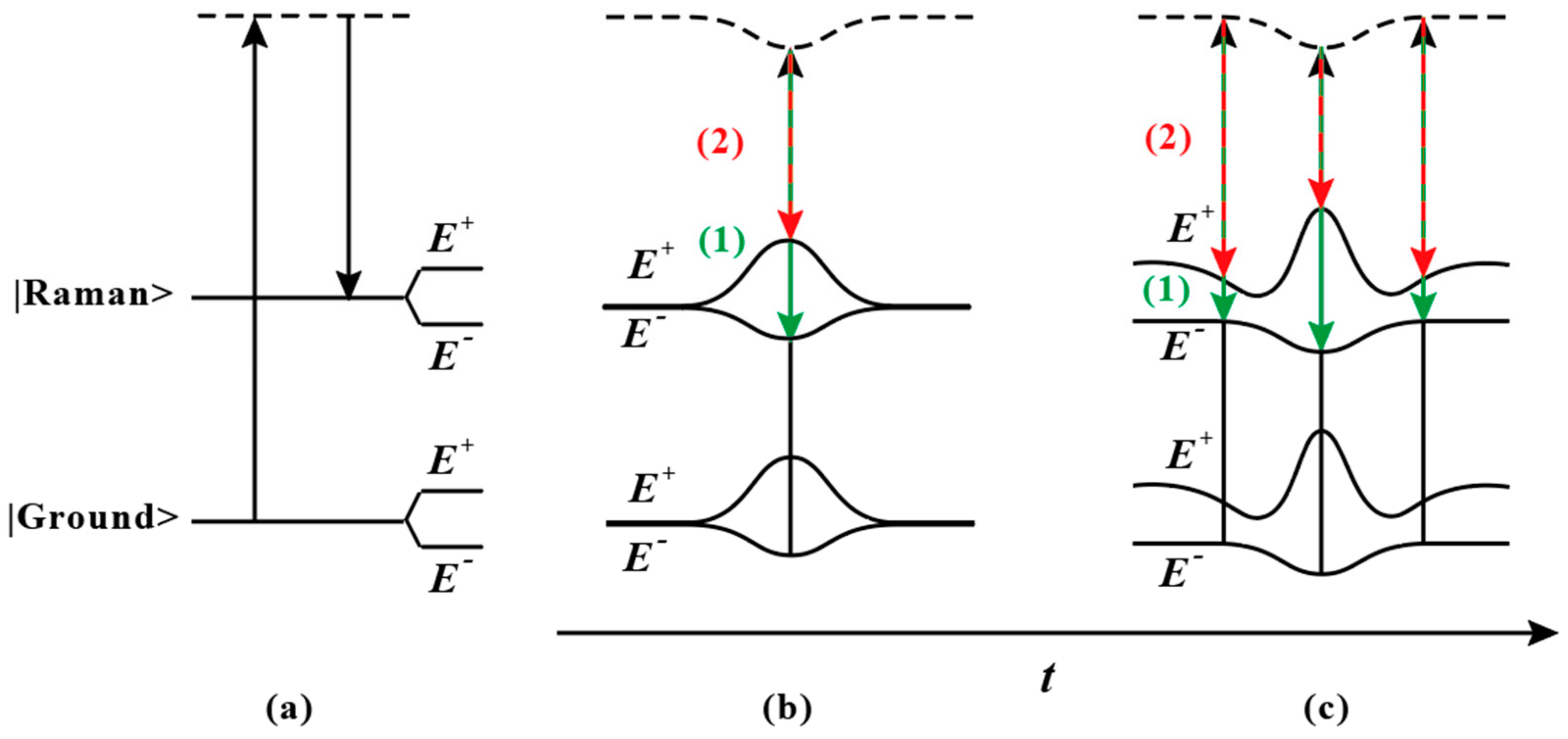
The work reported here demonstrates that the red-shifted spectral peak observed in transient MRG spectra has a spectral chirp that matches what would be expected from linear Raman scattering between manifolds of time-varying two-photon Stark-shifted states. The Hickman theory only allows for a closed system, with all the interactions coming from the third order, nonlinear process at the Raman frequency. This theory then does not account for the frequencies that could come from linear Raman scattering occurring between the lower energy state of one manifold and the higher energy state of another as depicted in
Figure 3. In
Figure 3a, we show the linear Raman process for the unshifted states having the same Raman frequency as the nonlinear Raman signal. Also shown in
Figure 3a are the Rabi frequency shifts of the molecular levels for the case of constant pump fields. In
Figure 3b,c, we show that if we assume that initially the population is in one state, which would be the E
− state for red-detuned pumps, then the linear Raman process could lead to two Stokes frequencies being generated between the dressed states.
For the time-varying coupled states, the frequency difference between the two Stokes pulses also then varies in time. In
Figure 3b, we show the Raman scattering between the shifted levels when the pump pulses overlap temporally. The pump pulse is depicted by a black arrow and population is pumped from the lower E
− level to a virtual level. The usual Stokes signal given by a shift of the Raman frequency is depicted by the green arrow and moves the population to the higher E
− level. The red-shifted Stokes pulse is depicted by a red arrow and takes the population to the higher E
+ level.
For the case of timed pump pulses, there are no shifts at early and late times. The arrows depict the maximum shift in frequency for the two Stokes pulses. Three different times during the pumping time are depicted in
Figure 3c, for the case of time-delayed pump pulses. The frequency of the usual Stokes pulse, given by the scattering between the E
− states, is constant and shifted from the pump frequency by the Raman frequency. We will therefore refer to this pulse as the Raman pulse. However, the second Stokes pulse will have a time-varying frequency with the maximum frequency difference between the two Stokes pulses occurring at the center time between the two pulses. We will refer to this pulse as the red-shifted pulse. In this case, due to the Stark shift, the frequency difference between the Raman pulse and the red-shifted pulse can be reduced from the frequency shift that caused by pump detuning. The frequency separation will again increase at the center because of the Rabi frequency shift. We only show the Stokes order being produced. This would imply that the red-shifted frequency observed on the first anti-Stokes comes from the red-shifted Stokes pulse pumped by the second anti-Stokes. We could have also shown linear anti-Stokes being generated if the pump pulse started on the upper manifold of states, causing two anti-Stokes pulses from transitions to either E
+ or E
− on the lower manifold. We cannot tell from our measurements which of these two linear processes is the dominant process.
In
Figure 4, we plot the modeled chirps of the two Stokes pulses for the case depicted in
Figure 3c. For this example, the Raman pulse has the same linear chirp as the pump pulse, and the red-shifted pulse has the same linear chirp with the addition of the time-dependent frequency shift from the generalized Rabi frequency. Far from the peak of the pulse, the red-shifted pulse has the same linear chirp that would result from 4-wave mixing of the two pump pulses.
4. Comparison of Experimental and Numerically Modeled Spectrograms
To compare with the experimentally measured FROG spectrograms of the first anti-Stokes order, we derived numerical spectrograms constructed from the model, where the first anti-Stokes order comprised two pulses generated through Raman scattering between the different dressed states as depicted in
Figure 3. We refer to the first pulse as the Raman pulse and the second pulse as the red-shifted pulse. We assumed that the fields, E
1 and E
2, of both pulses were Gaussian. Adding the two pulses together with an amplitude ratio
, and phases
and
, we can obtain the total electric field,
where
and
are the pulse durations,
is the central frequency of the Raman field, E
1. We are assuming that the Raman pulse is given by the pump pulse with the frequency shifted by the Raman frequency. Therefore, the phase
of the Raman pulse is taken to be the phase of the pump pulse. We also ensure that the phase at the peak of the Raman pulse is 0 so that we can impose a known phase difference between the two pulses. The phase
is given by the summation of the phase
, the phase given by the time integral of the time-dependent generalized Rabi frequency shift, described in Equation (1), and a constant phase difference.
We allowed there to be a constant phase shift of approximately π, added to the second pulse. In our initial attempts to model the spectrogram, we used a simpler two-pulse model, where the second pulse could have a different central frequency and we added a third-order phase to allow the central frequency separation to be larger from the peak intensity and we studied the case with maximum red-shifting. We allowed the two pulses to have different peak times and we noted that the optimized double pulse had a red-shifted pulse followed by the Raman pulse. The delay between the two pulses was about 1 ps and dispersion could not account for the red pulse coming ahead of the Raman pulse. Also, assuming that the Raman pulse would be timed to the pump pulses, we realized that this solution having a pulse appear before the pump pulse was unphysical. The appearance of a red pulse ahead of a blue pulse was most likely the result of two overlapping positively chirped pulses with a near π phase shift between them. With a π phase shift, a node would appear at the center of the combination of two pulses, with the red front half of the pulses appearing ahead of the trailing combined blue parts of the chirped pulses.
Upon closer examination, we concluded that the appearance of a red pulse preceding a blue pulse was likely a consequence of two overlapping positively chirped pulses with an almost π phase shift between them. With a π phase shift, a node formed at the center of the combined pulses, causing the red front half of the pulses to appear ahead of the trailing combined blue portions of the chirped pulses. This intriguing behavior shed light on the complex interplay of phase shifts and chirp effects in our experimental setup. The amplitude ratio between Stark shift and Rabi frequency depends on the polarizabilities, , , and as shown in Equations (2)–(4). In our experiment, the Raman medium is SF6, which has calculated values for , , and of 1.65456 × 10⁻³¹ m3, 1.64378 × 10⁻³¹ m3, and 1.66841 × 10⁻³¹ m3, respectively. With these values, we can determine that the amplitude ratio between the Stark shift and Rabi frequency is approximately 1:60. Hence, the Rabi frequency dominates the Stark shifting in SF6.
For the calculation of the intensity-dependent generalized Rabi frequency term, we assumed the pump pulses have Gaussian shape, with the experimentally measured pulse duration. The beam area was given by the diameter of the hollow fiber, which was 150 µm. We measured the energy before the hollow fiber and performed the experiments at three average energies of 1.2 mJ, 1.7 mJ, and 2.2 mJ. We also measured that ~30% of the light was transmitted through the fiber, with most of the loss coming from fiber coupling losses and Fresnel losses at both cell windows. In the model, we used the average energy before the fiber and used a variable energy coefficient to account for the losses and energy jitter of the laser.
To minimize the error between the experimental and modeled spectrograms, several of the variables were iterated. Within the generalized Rabi frequency term, we allowed the pump energy and time delay between pulses to vary around the average experimental values. This accounts for the experimental jitter of the laser in energy and time delay. In addition to these variables, we iterated the values of pulse durations T1 and T2, the amplitude ratio of the two fields, and the constant phase shift between the pulses. We compared the error with that given by the standard second harmonic FROG iteration and obtained comparable errors to the double-pulse model, even though we limited the profiles of both pulses to be Gaussian in the simulation.
We initiated our analysis by comparing the model’s predictions to experimental results obtained at a pump pulse delay of 333 fs, which corresponds to the point where the maximum number of Raman orders is generated. In this specific experimental run, we acquired three spectrograms for each energy setting. Notably, for the total pump energy of 2.2 mJ, one of the three spectrograms exhibited distinct characteristics compared to the other two. Strikingly, it closely resembled the spectrogram observed when the pump pulses were temporally synchronized. However, to obtain a result with minimal error for this spectrogram, the model required a significantly lower pump energy and a much smaller time delay between the pulses. We attribute this discrepancy to experimental timing and energy fluctuations, which can introduce variability into the measurements. For the other two pulse energies, the three measured spectrograms exhibited consistent patterns. The average FROG reconstruction errors across the three shots for the pump energies of 2.2 mJ, 1.7 mJ, and 1.2 mJ were 0.0059, 0.0058, and 0.0135, respectively.
To further gauge the accuracy of our model, we assessed the error between the double-pulse model predictions and the experimental spectrograms for the same three pulse energies. The resulting errors were 0.0064, 0.0056, and 0.0065, respectively. Throughout the nine shots, the average delay time was determined to be 357 fs, with a standard deviation of 72 fs. This standard deviation aligns with our experimental timing accuracy and jitter, reflecting the precision of our timing measurements.
Additionally, the average pump energy used in the model to calculate the generalized Rabi frequencies was found to be 0.52, 0.75, and 0.98 for the cases with pump energies of 1.2 mJ, 1.7 mJ, and 2.2 mJ, respectively. These model-predicted energies corresponded to approximately 43%, 44%, and 45% of the measured energies before the fiber. This alignment is reasonably consistent with the 30% measured energy output, with the understanding that some energy loss may occur at the exit window. Moreover, it is worth noting the presence of white light emitted along the length of the fiber, which means our measurements represent an average of the energy distributed along the fiber. This characteristic introduces an additional layer of complexity to our analysis, as we must consider this distributed energy when interpreting the results.
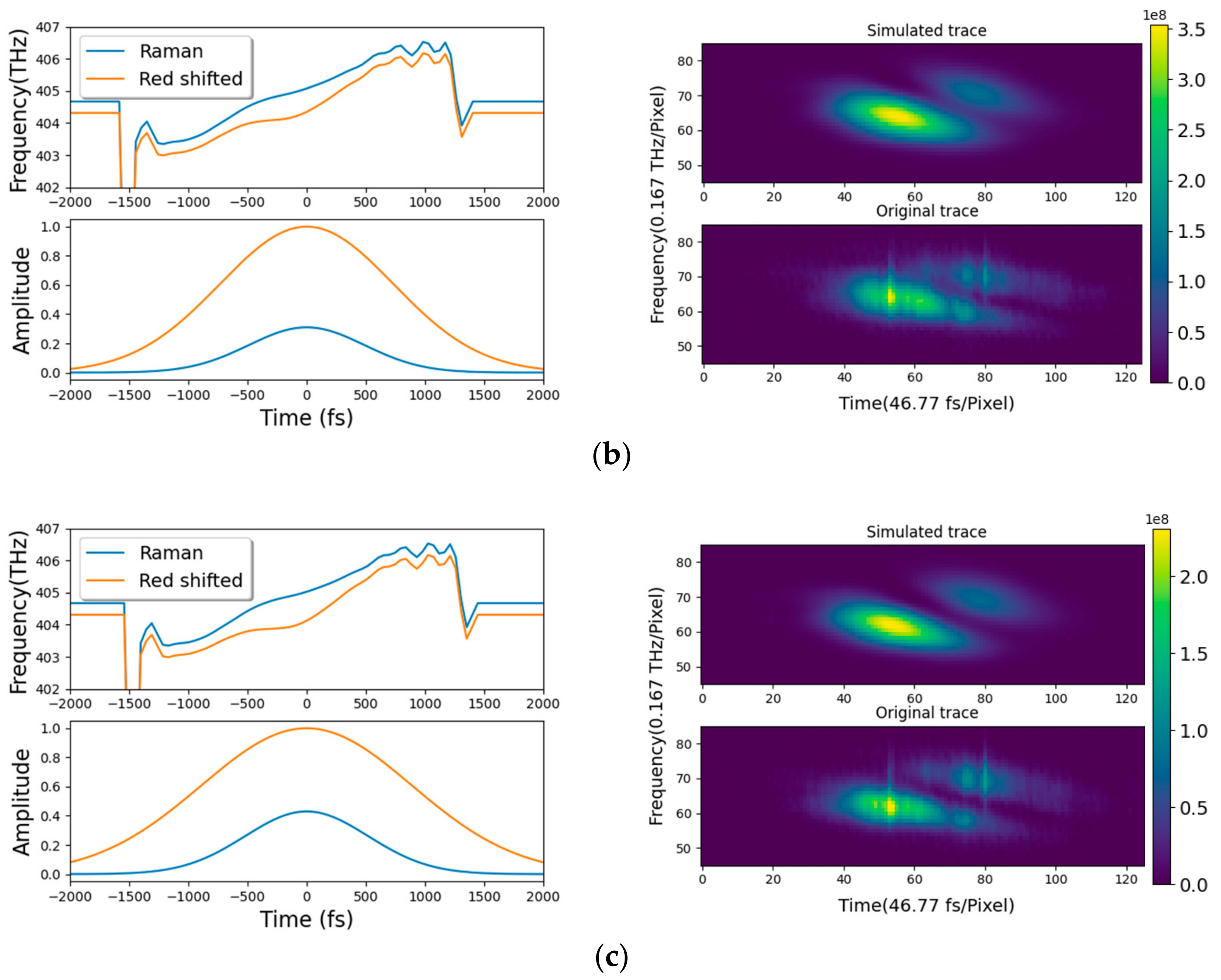
Shown in
Figure 5 are the optimized, simulated chirps of the two pulses comprising the first-order anti-Stokes order, along with the simulated pulse profiles. Also shown are the experimental and simulated spectrograms. In
Figure 5a–c, we show the results of one of the shots for experimental pump energy of 1.2, 1.7, and 2.2 mJ, respectively. The optimized simulated results in
Figure 5a correspond to a pump energy of 0.52 mJ and a pulse delay of 414 fs. The Raman pulse had a duration of 884 fs and the red-shifted pulse had a duration of 1429 fs. The amplitude of the red-shifted shoulder was 100 times larger for this case. The phase difference was 3.12. The average results for the three sets of profiles gave a Raman pulse duration of 872 fs, a red-shifted pulse duration of 1356 fs, an amplitude ratio of 14 and phase difference of 3.14. The optimized simulated results in
Figure 5b correspond to a pump energy of 0.76 mJ and a pulse delay of 359 fs. The Raman pulse had a duration of 848 fs and the red-shifted pulse had a duration of 1010 fs. The amplitude of the red-shifted shoulder was 4.2 times larger for this case. The phase difference was 2.76. The average profiles for the three spectrograms gave a Raman pulse duration of 831 fs, a red-shifted pulse duration of 1084 fs, an amplitude ratio of 5.3, and phase difference of 2.84. The optimized simulated results in
Figure 5c correspond to a pump energy of 1.0 mJ and a pulse delay of 365 fs. The Raman pulse had a duration of 865 fs and the red-shifted pulse had a duration of 1485 fs. The amplitude of the red-shifted shoulder was 2.3 times larger for this case. The phase difference was 2.99.
As can be seen in
Figure 5, the simulated spectrograms match well with the experimental measurements. The chirp of the Raman pulse is given as the chirp of the pump pulse that does not have a perfect linear chirp. It is worth noting that we first modeled the Raman as having a linear chirp that closely matched the pump chirp and that the red-shifted pulse chirp included the same linear chirp but the error between the model and the experiment was not as low as the FROG traces in many cases and so we decided to use the actual pump pulse chirp as measured by the FROG and we were able to reduce the error between the modeled and measured spectrograms.
In our second series of experiments, we aimed to investigate how the instantaneous frequency separation of the pump and Stokes pulses affected the spectrum of the first anti-Stokes order.
Figure 6 illustrates the results of these investigations, featuring both simulation outcomes and experimental measurements. Specifically, we focused on three distinct time delays: 0 fs, 333 fs, and 666 fs, all conducted at the average pump energy of 2.2 mJ. For each time delay, we conducted 11 spectrogram measurements. The average errors from FROG reconstructions were as follows for the increasing time delays: 0.0094, 0.0082, and 0.0048, respectively. Meanwhile, the double-pulse model yielded errors of 0.0087, 0.0085, and 0.0054 for the same time delays.
Interestingly, the average simulated pump pulse energy across all 33 spectrograms taken during this entire run was 0.76 mJ, which corresponds to just 35% of the expected 2.2 mJ. This discrepancy suggests that coupling losses were likely higher during this experimental run. The simulated chirps, as displayed in
Figure 6, indicated slight differences in pump pulse chirp compared to the energy scan experiment.
Across the three cases, the average time delays were approximately 58 ± 18 fs, 345 ± 8 fs, and 709 ± 43 fs. The average durations of the Raman pulses closely matched the experimental pump duration, measuring 780 fs for each case. Regarding the red-shifted pulses, their average durations were found to be 1340 fs, 1018 fs, and 1375 fs, respectively, all exceeding the duration of the Raman pulses. The amplitude ratios between the red-shifted and Raman pulses averaged at 0.83 ± 0.20, 1.40 ± 0.70, and 5.50 ± 2.70 for the increasing time delays. Additionally, the average phase differences between these pulses were 0.43 ± 0.25, 4.10 ± 0.90, and 6.22 ± 0.29, respectively.
Figure 6a shows the results for a case with nominally timed pump pulses. For the depicted case, the optimized simulate results gave a pump energy of 0.75 mJ with a delay of 19 fs. The Raman pulse had a duration of 795 fs and the shifted pulse had a duration of 1389 fs. The amplitude of the red-shifted pulse was 0.86 compared to the Raman pulse. The phase difference between the pulses was 0.67.
Figure 6a shows the results for a case with nominally timed pump pulses. For the depicted case, the optimized simulated results gave a pump energy of 0.75 mJ with a delay of 19 fs. The Raman pulse had a duration of 795 fs and the shifted pulse had a duration of 1389 fs. The amplitude of the red-shifted pulse was 0.86 compared to the Raman pulse. The phase difference between the pulses was 0.67.
Figure 6b displays the results having a pump energy of 0.74 mJ with a delay of 343 fs. The Raman and shifted pulses had durations of 768 fs and 981 fs, respectively. The amplitude of the red-shifted pulse was 1.6 times larger than that of the Raman pulse. The phase difference between the pulses was 4.26. The result for the longest time delay is shown in
Figure 6b. For this shot, the pump delay was determined to be 683 fs mJ and the pump energy was 0.74 mJ. The Raman and shifted pulses had durations of 818 fs and 1182 fs, respectively. The amplitude of the red-shifted pulse was 5.6 times that of the Raman pulse and the phase difference between the pulses was 0.43.
5. Discussion
As discussed in the Introduction, a second harmonic FROG iteration program does not give unique results for complicated electric fields. We were not able to obtain consistent FROG results for the different shots with the same experimental conditions and so we looked for a different method to glean the electric field from the measured spectrograms. We first tried simple double-pulse models that had the Raman pulse with a simple linear chirp and the shifted pulse having a central frequency shifted by some amount and third-order phase to account for a time-varying frequency separation. This gave unphysical results. We then used the theoretical model for the generalized two-photon Rabi frequency-shifted dressed states, included in the theory describing MRG. We looked to see if the complicated measured spectrograms would give more consistent results, if we assumed one of the pulses came from the normal Raman scattering process and a second pulse was generated through Raman scattering between the phased and anti-phased dressed states. This model did indeed give more consistent results for each of the experimental conditions and the changes in the red-shifted pulse corresponded to what would be expected with the model.
As can be seen in the plots of pulse chirps shown in
Figure 5, with increasing pump energy, there is an increasing dip in the frequency of the red-shifted shoulder at half the pump pulse delay, corresponding to the time of the maximum generalized Rabi frequency. The pump energy derived in the model for the three different energy cases varied by the same ratios as the experimental values. The simulated pump energy was 0.44 of the energy measured before the pressure cell containing the hollow fiber and so this value is very close to the experimental value. The average time delay across all nine shots for this run was 357 ± 72 fs which falls within the experimental accuracy and jitter levels.
The results shown in
Figure 6 show that the frequency difference between the pulses near the peaks of the pulses at time zero does not change much as the pulse delay increases. Rather, the shape of the frequency chirp of the red-shifted pulse changes significantly. For the timed case, shown in
Figure 6a, the optimized numerical result shows that the two pulses are overlapped spectrally until the intensity of the pulses becomes significant. This is expected from the model, as there is zero total detuning at the edges of the pulse because the pump pulses are resonant with the Raman transition and the generalized Rabi frequency would be zero. We also see the maximum dip in frequency in the red-shifted pulse at the center for the timed case as expected, because both the Stark shift and the on-axis Rabi shift are maximized in this case where the two pump pulses coincide. It can be seen in
Figure 6, with increasing time delay, that the frequency shift between the pulses at early and late times increases with increasing delay between the pump pulses and the frequency dip both decreases and occurs further from the peak of the pulses. At the longest time delay shown in
Figure 6c, the two pulses resemble what would be seen if the second pulse came simply from four-wave mixing as the overlap of the two pulses is small, resulting in low Rabi frequency shifts.
The simulated results show good agreement between the simulation and the experimental results and so indicate that the secondary pulses are indeed a result of Raman scattering between the dressed states. The simulations also give pulse profiles and phase differences between the pulses that we cannot yet address with the theory of Raman scattering between different dressed states. We have not carried out a theoretical calculation that could elucidate a possible p phase shift. We expect it could be a result of the Raman pulse being caused by scattering between like states and the red-shifted pulse coming from scattering between phased and anti-phased states. We also do not yet have a theory that can account for the effects of propagation resulting in further conversion from the first anti-Stokes to higher-order anti-Stokes as well as conversion to Stokes orders. We expect this propagation to influence the pulse profiles. The propagation would also affect the phase between the two pulses because they have different central frequencies and so would propagate at different speeds because of dispersion.
In all six cases shown in
Figure 5 and
Figure 6, the Raman pulse duration matches the pump pulse duration. This would be expected for linear Raman scattering. However, the MRG process relies on nonlinear Raman scattering. The shifted shoulder is consistently longer in duration than the Raman pulse and, except for the timed case, is higher in amplitude than the Raman pulse. The higher amplitude of the red-shifted pulse with a time delay of 333 fs is consistent with the observations in our earlier work [
10], which showed that the amplitude of the red-shifted peak grew with increasing anti-Stokes order until there was only the shoulder at the highest orders for this time delay between pump pulses. We expect that this is due to the pump pulse instantaneous frequency separation being on resonance with the dressed states for this delay time. This increase in amplitude of the red-shifted pulse with increasing order could account for the longer pulse duration of the red-shifted pulse because the nonlinear stimulated Raman scattering for this frequency separation would decrease the high-intensity peak more than the wings as the anti-Stokes pulse is converted to the next higher anti-Stokes through nonlinear Raman scattering.
