An Integrated Approach to Leak Detection in Water Distribution Networks (WDNs) Using GIS and Remote Sensing

Abstract

Leakages in the water distribution networks (WDNs) are real problems for utilities and other governmental agencies. Timely leak detection and location identification have been challenges. In this paper, an integrated approach to geospatial and infrared image processing was used for robust leak detection. The method combines drops in flow, pressure, and chlorine residuals to determine potential water leakage locations in the WDN using Geographic Information System (GIS) techniques. GIS layers were created from the hourly values of these three parameters for the city of Sharjah provided by the Sharjah Electricity, Water, and Gas Authority (SEWA). These layers are then analyzed for locations with dropped values of each of the parameters and are overlaid with each other. In the case where there were no overlaying locations between flow and pressure, further water quality analysis was avoided, assuming no potential leak. In the case where there are locations with drops in flow and pressure layers, these overlaying locations are then examined for drops in chlorine values. If overlaying locations are found, then these regions are considered potential leak locations. Once potential leak locations are identified, a specialized remote sensing technique can be used to pinpoint the leak location. This study also demonstrated the suitability of using an infrared camera for leak detection in a laboratory-based setup. This paper concludes that the following methodology can help water utility companies in the timely detection of leaks, saving money, time, and effort.

1. Introduction

Water distribution networks (WDNs) are complex systems that are prone to significant water loss, and this loss is mainly due to pipe leakage [1,2]. It is estimated that leaks can contribute up to 70% of water losses in transmission systems [3]. Leakages in these WDNs are mainly caused by pipe damage or by the network’s inability to control pressure due to uncertain demand and operating conditions [4]. Leaks in pipelines are an issue of increasing concern in WDNs as they have negative environmental, economic, and social impacts. Pipe leakages have detrimental effects on natural water resources, nearby infrastructure, and the environment, as they cause pipes to burst and enable the entry of harmful contaminants into the network [4,5]. The loss of a substantial volume of water that has undergone costly treatment is, for one, a serious economic issue [6]. Moreover, leaky pipes cause an increase in pumping energy and system rehabilitation costs, which compromise water quality by enabling the entry of contaminated groundwater, pathogens, and soil constituents [7]. Leaks also have the potential to erode soil and recharge aquifers beneath urban areas, which puts building foundations at risk [8]. Not only will mitigating leakages reduce operating costs and increase revenues, but it will also improve water efficiency, minimize infrastructure damage, and prevent adverse effects on human health [9].

Detecting these leakages poses a great challenge to engineers since the pipes are usually buried underground. For this reason, constant monitoring is required to identify and prevent potential water leakages in pipes. Traditional leak detection methods, which are disruptive techniques, would change the structure of the WDN, disrupting the serviceability of the network [10]. However, research on novel non-destructive methods has shown the potential for leak detection without altering the chemical composition or geometry of the materials being investigated.

The advent of technology has led to developments in non-destructive leak detection techniques for WDNs. For instance, innovative non-destructive techniques (NDT) like infrared (IR) cameras, spectrometers, and ground penetration radar (GPR) have been used to identify leaks in different types of pipes at different moisture contents [10,11]. The study deduced that all three NDTs could identify leaks in PE, PPR, and PVC pipes, but the detection effectiveness decreased as the moisture content of the soil increased. A recent study has shown the use of GPR and IR cameras simultaneously to effectively determine water leaks in both cold and hot weather conditions [12]. Since GPR is a geophysical imaging technique used for subsurface monitoring, it can accurately identify the pipe’s location underground [12]. The IR camera is then able to determine leakage locations and estimate the leakage area [12]. Thermal imaging has also been successful in leak detection [12,13]. In addition, acoustic emission methods are another NDT suitable for detecting leaks, as they collect sound signals generated by the cavitation and turbulence that occur in a leak [14,15]. It is important to note that signal processing and classification methods are required to verify that the noises formed are due to leaks [14]. Therefore, integrated approaches are proven to be the most effective for accurate and efficient real-time monitoring. Therefore, using a combination of NDTs has proven to enhance the effectiveness of leak detection methods to help mitigate leakages. Several studies have proposed techniques for leak detection in pressurized transmission mains (TMs). These techniques can be used on WDNs as well; however, more studies are focusing on TMs as the current technology for fault detection on TMs is lacking [16]. This issue is being addressed because research has shown that TMs with relatively larger diameters have larger leaks than expected, and the costs of replacing deteriorating TMs are higher than those of WDNs [17]. A study by [16] explored the use of transient tests, such as Transient Test-Based Techniques (TTBTs), for fault detection in water transmission mains. This technique involves inserting a small pressure wave into a pipeline, which travels through the pipeline, detecting leaks, partial blockages, and the reduction of the pipe wall’s thickness due to corrosion. The study illustrated the successful usage of TTBTs in a real-life pipe system. Another study designed a smart-portable pressure wave maker (S-PPWM) for leak detection in TMs as a form of TTBT [17]. The design was built to minimize the TM volume and to ease the evaluation of the minimum detectable leak for a given TM. The device has been proven to be used within leak detection surveys of TMs based on the execution of safe transient tests (TTBTs) [17].

The reviews of existing leak detection methods indicated the problem of accuracy in identifying the location of leakages. Therefore, combining different technologies to improve the accuracy of leak detection has proven to be most effective [18]. Recent studies have explored the use of geographic information systems (GIS) and remote sensing for different practical applications. One study by [19] developed a database of morphometric characteristics and their hydrological implications using a satellite image of the Jimen basin located in northern Iraq. The study evaluated the effect of solar radiation on the basin’s surface runoff, allowing them to predict the presence of saturated soil for water harvesting [19]. In addition, a study conducted in southwest Saudi Arabia integrated GIS and remote sensing to determine the hydrological characteristics of a watershed in Saudi Arabia [20]. The paper’s findings serve as a basis for practical applications in flood management and water harvesting [20].

This paper aims to use GIS and remote sensing with an infrared camera to accurately detect leakage in a pipe network. GIS refers to a computer-based system that stores, analyzes, and displays geographically referenced data [21]. Therefore, GIS is essential for the operation of water networks; studies have shown the integration of GIS can assist in real-time leak detection [22,23]. A study by [23] employed the use of GIS to help water utility companies predict and assess vulnerable locations prone to leakage in WDNs. Another study [24] utilized the ArcGIS software 3.2 to assist in the analysis of water losses in a WDN by using four feature classes: pipeline layer, meter layer, elevation map, and field operations layout. ArcGIS displayed the results obtained from the field and the results calibrated, which illustrated the faulty meters and pipe leak locations [24]. Combining the results of the model displayed on GIS with other layers, like a topographic layer of the region or district metered area zones, enhanced the analysis of critical zones of WDNs for optimal operation and management of the network [24].

Remote sensing provides better temporal and spatial coverage than ground detection methods [25]. Recent studies have shown that spatial resolution is an essential parameter for the detection and mapping of water leakage regions using remote sensing data. A study [18] identified leakages by recording remote sensing data from ground spectroradiometers and hyperspectral data from a low-altitude system. The study deduced that water leakages can be monitored and detected using the appropriate spatial resolution images. The spectral signals of dry and wet soils were recognizable in the visible range of 400–700 nm and in the near-IR range of 750–900 nm [18]. In comparison to dry soils, wet soils have 20–25% lower reflectance values, and the difference is maximized in the near-IR range [16]. The research study concluded that remote sensing is effective for the determination of water pipe location and leakage [18].

The literature on using hyperspectral imaging for water leakage detection is limited; however, it is a growing area in remote sensing [26]. Hyperspectral imaging is a developing technology in remote sensing where an imaging spectrometer collects hundreds of images at different wavelengths for the same spatial area [26]. It is concerned with the measurement, analysis, and interpretation of spectra taken from a given scene or object at a short, medium, or long distance by an airborne (drone) or satellite sensor [27]. The NASA Jet Propulsion Laboratory’s Airborne Visible Infra-Red Imaging Spectrometer (AVIRIS) can record the visible and near infrared spectrum (wavelength range 400–2500 nm) of the reflected light on an area 2–12 km wide and several kilometres long using 224 spectral bands [28]. The result is a stack of images whereby each pixel has a corresponding spectral signature, or ‘fingerprint’, that distinguishes the underlying objects, and the final data volume comprises several gigabytes per flight [26]. This usually requires hardware accelerators to speed up computations. Hyperspectral sensors are expected to increase their spatial, spectral, and temporal resolutions [26]. The incredible amount of spectral information available from the latest hyperspectral devices has opened doors to real-time processing applications such as monitoring leakages [29].

An IR camera detects infrared energy reflected or emitted by an object and converts it into a thermal image [10]. Leaks in an underground water network may change the temperature of the surrounding soil, as leaked water is typically cooler than soil, which absorbs thermal energy faster than water [10]. In addition, IR cameras can be used at any time of the day, and they can investigate large areas in comparatively less time with lower costs than other NDTs [30]. The paper presented the use of a thermography IR camera for the detection of heat changes at pavement surfaces due to water pipe leaks underneath the surface. The results of the study showed that the IR camera successfully detected several leaks as thermal contrast at pavement surfaces occurred in the fall and spring seasons. However, it failed to detect leaks during the summer and winter due to high pavement temperatures and snow coverage. A more recent study evaluating the effectiveness of spectrometers, GPR, and IR as NDTs deduced that the IR camera was shown to be the most effective for pipeline leak detection [10].

A study [31] used medium- and high-resolution data from different satellites for the detection of water leakages in the “Frenaros—Choirokoitia” water pipe in Cyprus. The study applied two alternative methodologies. The first used a high-resolution QuickBird image to identify and verify ‘suspicious leaks’ in a small area near the water pipes [31]. The second methodology involved using multi-temporal analysis using medium-resolution SPOT images. The analysis focused on regions around the joints of the pipe, using a 10-meter buffer zone [31]. This method recorded 10 possible leakage points along the 25-kilometer-long pipeline [31]. The effectiveness of this study could be enhanced if the images were taken of a larger area, displaying an entire WDN and not just a single pipeline. In addition, acquiring images at a high spatial resolution can increase the accuracy of leak detection along the pipeline.

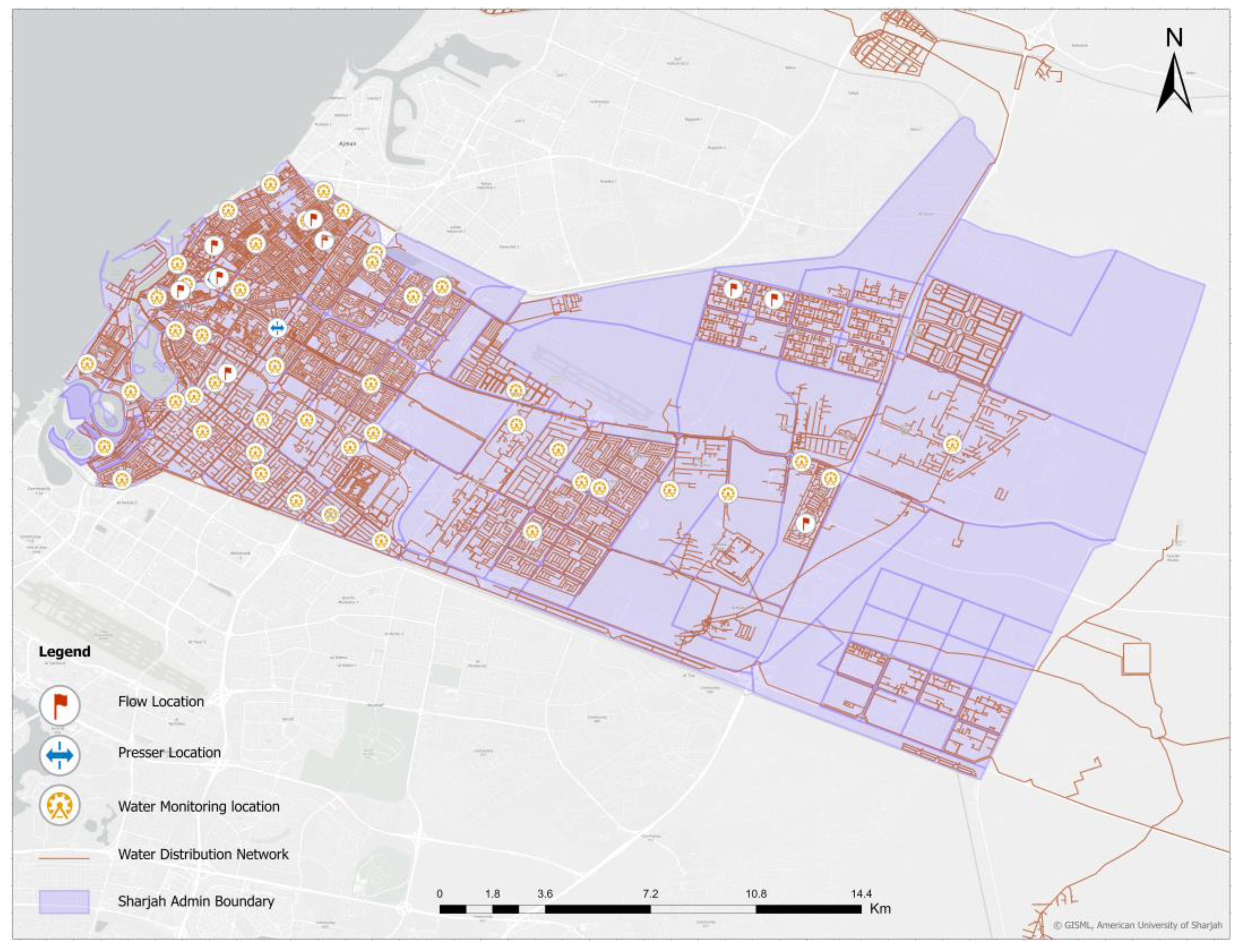
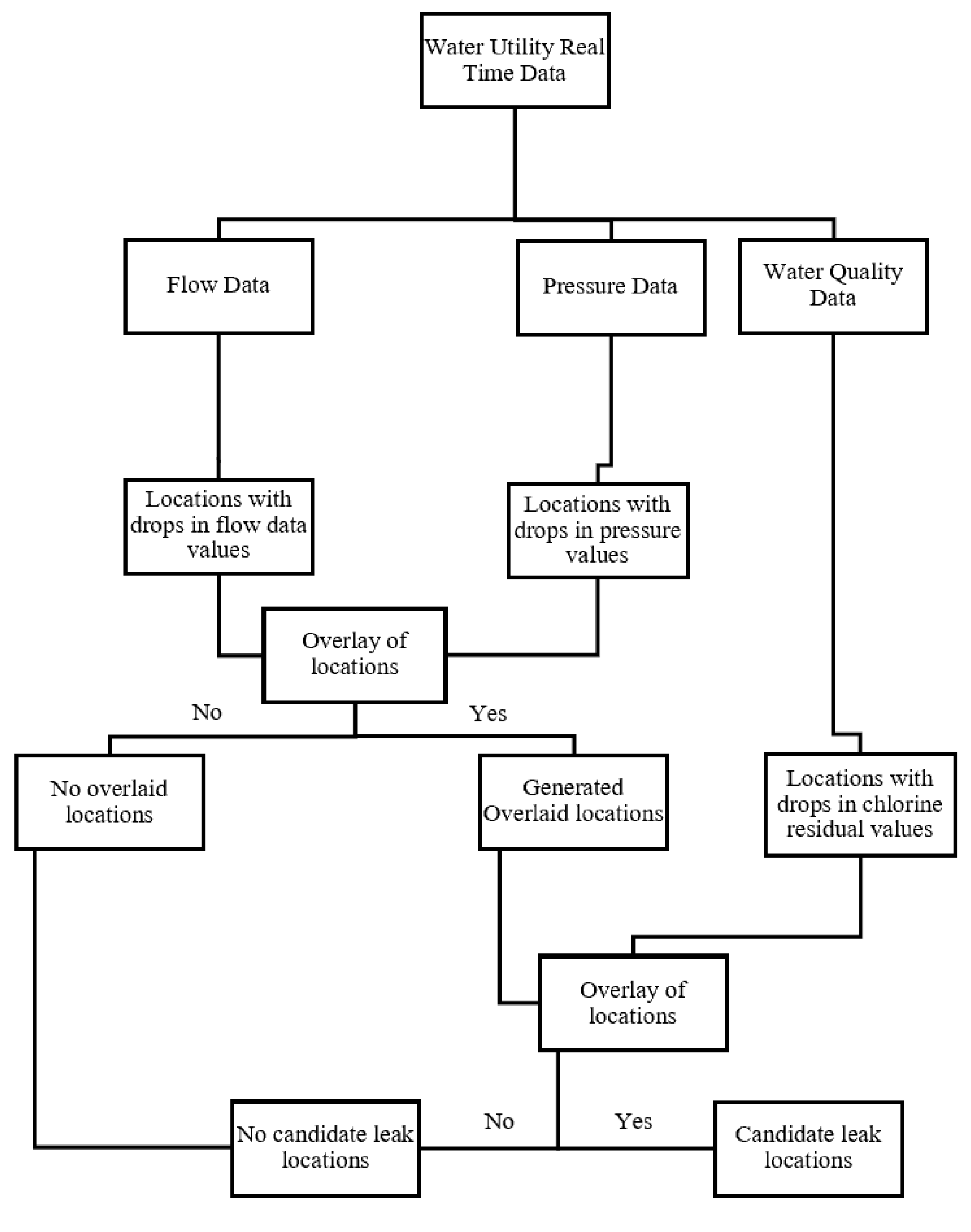
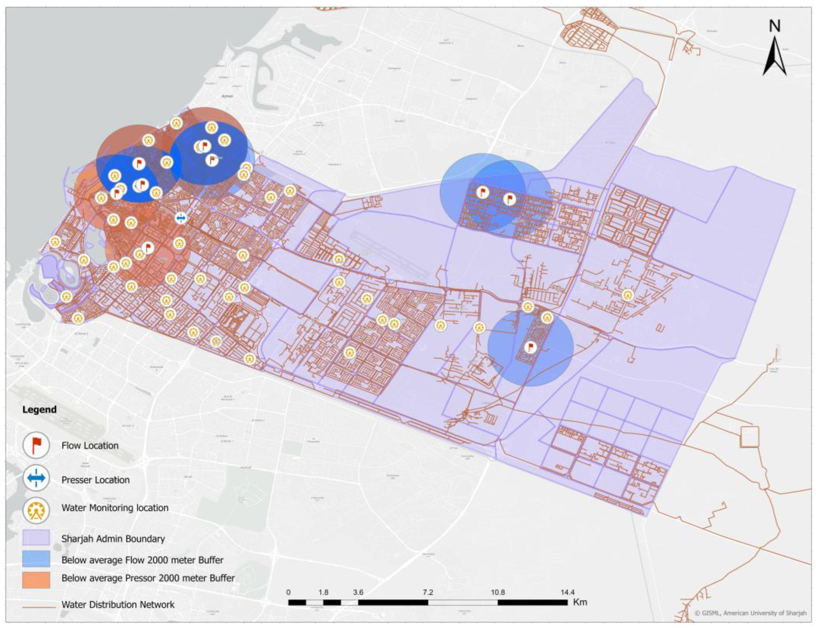
In this paper, an integrated approach of GIS and IR image processing was used to detect leakages in the WDN of Sharjah Electricity and Water Authority (SEWA). The objective of this paper is to develop a leak detection method using GIS and remote sensing. The aim of using this method is to enhance the efficiency of WDNs by increasing their accuracy in identifying leakages. This study creates a GIS-based customized system to identify potential leakage locations and deploys an IR camera to identify potential leak locations. The main contributions of this paper are as follows:

• For potential locations of leak identification, we used GIS analysis methods, including buffer and intersection methods, using drops in water pressure, flow, and chlorine values.
• Capturing infrared drone images for the potential leak locations identified through the GIS analysis methods.
• Use of log ratio methods to process the infrared drone images for robust leak localization.

2. Materials and Methods

To achieve the objectives, the paper develops an integrated leak detection method using GIS and remote sensing. For this reason, the methodology is deconstructed into two phases. In the first phase, the use of GIS helps identify potential leak locations using different sets of hydraulic and water quality data from a real WDN that may indicate potential leaks. That is, sudden drops in pressure, flow, and water quality can be shown on spatial variability maps generated by GIS. At the end of the first phase, either no leaks were found in certain locations or candidate leak locations were identified. Once the candidate leak locations are found, the second phase begins with the use of remote sensing to capture and process images that can be utilized at the candidate leak location.

2.1. Phase 1: GIS Application

In this study, WDN for the City of Sharjah, UAE, was used to demonstrate the applicability of the model. Sharjah Electricity and Water Authority (SEWA) manages the desalination plants and WDN in the City of Sharjah. The WDN consists of more than 4000 km of pipe networks. Figure 1 illustrates a map of SEWA’s WDN that was used for the GIS-based model for the leak detection system. Most of the pipes were made of asbestos-cement pipes. The SEWA installed many sensors throughout the large WDN to monitor the hydraulic and water quality parameters to ensure enough water is available in good quality.

SEWA installed sensors in the WDN capable of monitoring real-time hydraulic and general water quality parameters. Potential leaks can cause drops in parameters like pressure, flow, and water quality. In addition, the larger the number of joints along a pipe length, the more likely it is for there to be a leak. In large WDNs like Sharjah, it is difficult to differentiate leaks from other sources of parameter fluctuations. Therefore, spatial variability maps were generated in GIS for pressure, flow, and water quality parameters such as pH, conductivity, and chlorine residuals. The spatial variability maps were used to identify parts of the WDN where large drops of pressure, flow, and chlorine residuals occur. It is assumed that locations with high drops in pressure, flow, and chlorine residuals may indicate potential leakages. Three conditioning factors were represented as raster layers on the ArcGIS Pro 3.2 software: pressure, flow, and chlorine residual.

The ArcGIS Pro software was used in this phase. The flow chart illustrated in Figure 2 shows the values of the three parameters—flow, pressure, and water quality—at a set of locations during any period. This data was provided by SEWA. The real-time data is continuous, and the software is expected to run analysis as data is provided. Initially, the flow and pressure parameters in different regions undergo overlay analysis. An overlay analysis carries through all the attributes of the features taking part in the overlay and creates a new polygon dataset. The data set provided ten locations (regions) in Sharjah and tabulated thirty readings for pressure and flow data for each location, and the average value was calculated for each of those data sets. Any individual value lower than the average of the data set is suspected of containing a leak. Each value indicating a drop in pressure or flow along the pipe was overlaid in the software, and this either created new overlaying regions or no regions at all. In the case where there are no overlaying regions among the two parameters, there is no need to analyze the water quality values, and the conclusion is that there are no leaks detected in the given set of locations at a particular time. In the second case, where there are one or more overlaying regions formed among pressure and flow drops, these overlaying regions are merged with locations that indicate drops in chlorine residual values. Afterwards, there is no new overlaying region, which indicates that there were no leaks in that location at a certain time or that new overlaying regions had formed. If one or more new overlaying regions are generated, then the conclusion is that those locations do have leaks. The proposed methodology uses ArcGIS Pro as well as a module builder based on Python code (Appendix A) to identify leakage locations.

2.2. Phase 2: Remote Sensing with an Infrared Camera

In the second phase of this integrated approach, thermal images (thermograms) of the model distribution system were captured using the FLIR420 thermal imaging camera, Wilsonville, Oregon, U.S. (Figure 3). The camera has a wavelength range of 7500–14,000 nm. On the right side of the camera’s display, the color range represents the temperature range of the captured area. The darker colors illustrate regions with lower temperatures, while the brighter colors illustrate regions with higher temperatures.

Since the data provided by SEWA was a few years old at the time of the study, conducting field tests may not be meaningful as maintenance activities might have already been carried out at the suspected locations. In addition, due to government restrictions related to field experiments at the locations identified in Phase 1, similar experiments were conducted on the model setup. The thermal images of the model water distribution system, shown in Figure 4a,b, were captured manually. This WDN model is a carefully built setup that includes a dune-sand-filled box with four PPR pipes (th = 5.7 mm) and is designed to simulate pipe leaks in underground conditions. One of the pipes is a regular pipe without any leaks, and the three other pipes were created with simulated leaks from cracks, holes, and joints. An experiment was conducted on the pipe with a hole. These grayscaled IR images generated during laboratory-based experiments were then processed to clearly display the heat signatures. Since water has a cooling effect compared to the surrounding soil, with the help of time series images, the leakage locations can be identified.

The aim is to capture the thermograms in grayscale RGB (red, green, and blue) format where all three layers are equal. Therefore, only one layer is selected for image processing. The grayscale image is later processed to a false color image with multiple layers for perception purposes to increase the contrast of the thermal images. Figure 5 and Figure 6 show a sample grayscale image and its corresponding false-color thermogram from a previous study [13]. The leakage is characterized by a lower temperature than the soil. It is important to consider that the temperature of the soil will vary with time. The temperature of the surrounding soil will decrease continuously as the leak spreads throughout the soil. Therefore, the surface with the highest temperature variation is above the leakage. The next section outlines the mathematical model that will emphasize the temporal temperature variation.

3. Results and Discussion

3.1. GIS Application

3.1.1. Case Scenario 1: No Detection of Leakage Location(s)

To prove that this integrated approach works, this method was applied to dates that are known not to have any leakages. The raw data provided by SEWA is shown below, and it illustrates the flow and pressure values for each day in one month at 10 locations in the city of Sharjah. Using ArcGIS Pro, the flow and pressure data for each location are evaluated to map the water quality parameters. As mentioned in the previous section, the assumption is made that any flow higher than the average or pressure value lower than the average from the data set (highlighted in green and red) is suspected to have a leak in that location. Another assumption for suspected leakage is customer complaints.

Table 1. Flow data provided by SEWA (first half of the month).

DMA	D1	D2	D3	D4	D5	D6	D7	D8	D9	D10	D11	D12	D13	D14	D15	D16
Al Rahmanya-1	740	760	660	680	710	770	710	670	600	790	580	740	500	600	0	650
Al Rahmanya-3	960	1100	1030	970	1200	1140	1210	1120	600	1160	990	1190	1140	670	1250	1210
Industrial Area-4	4500	5070	5440	6930	5430	5450	5120	5110	4760	4730	4960	5180	5380	5150	5150	5350
Industrial Area-4	30	20	10	0	40	30	40	40	20	10	0	10	20	40	10	30
Barashi	410	570	160	630	670	930	1180	2260	2070	1800	1220	1420	640	780	1060	830
Maysaloon	440	650	800	450	170	100	240	1310	1710	2540	2780	3120	2620	2670	2940	3110
Al Fayah	980	980	1020	970	1030	1050	1070	1080	1010	1060	1060	1080	1070	1060	960	1020
Al Ghuwair	3340	4230	8190	3800	4650	5290	2870	3850	830	790	870	860	1200	890	950	1070
Bu Tina	6500	6490	6600	7280	7270	7120	7010	7040	6930	7410	7800	7420	7410	7150	7200	7150
Al Sabkha	3740	3730	3690	3670	3770	3760	3680	3730	3700	3870	3810	3720	3840	3970	3780	3830
Al Sabkha	890	880	900	830	800	860	740	880	850	820	800	730	640	690	700	630
Al Ghaphia	1270	1140	750	220	550	1170	610	830	1060	740	350	690	830	730	850	760
Al Ghaphia	1160	1070	950	780	860	1070	930	1060	1050	800	680	740	650	640	750	750

and

Table 2. Flow data provided by SEWA (second half of the month).

DMA	D17	D18	D19	D20	D21	D22	D23	D24	D25	D26	D27	D28	D29	D30	D31
Al Rahmanya-1	660	780	600	730	720	660	660	670	600	680	640	710	670	560	710
Al Rahmanya-3	1180	900	1000	1270	1200	1210	1150	1390	1010	1180	1140	1230	1160	1200	1360
Industrial Area-4	5310	5180	5060	5340	5090	5220	5330	5250	4830	4950	5380	5160	5350	5380	5000
Industrial Area-4	30	40	20	0	10	20	20	30	80	110	50	80	60	60	80
Barashi	660	1260	920	970	1690	1370	1160	820	1220	1580	2070	1580	1710	1480	1270
Maysaloon	2850	2850	2190	1870	2090	2380	2390	2020	2650	2000	1740	0	1530	1400	1380
Al Fayah	1050	1050	1130	1010	1050	980	1010	990	1030	1170	1040	1060	1100	1020	1090
Al Ghuwair	1060	1050	950	950	940	920	980	950	1150	1450	260	210	210	220	200
Bu Tina	7040	7690	7380	7070	6950	6860	7050	7070	7320	7380	7200	7220	7470	7220	7150
Al Sabkha	3790	3860	3790	3790	3760	3700	3770	3700	3730	3750	3680	3690	3780	3750	3770
Al Sabkha	620	670	690	710	720	770	750	720	700	640	620	630	630	680	740
Al Ghaphia	640	160	60	360	730	750	900	780	460	510	550	440	230	180	550
Al Ghaphia	790	720	720	810	800	800	920	760	910	800	770	830	750	740	820

show the daily flow data (in m³/day) at 10 different locations in a specific month, and

Table 3. Average flow in a month (m³/day).

DMA	AVG (m3/day)
Al Rahmanya-1	651.9354839
Al Rahmanya-3	1113.548387
Industrial Area-4	5210.967742
Industrial Area-4	33.5483871
Barashi	1173.870968
Maysaloon	1773.870968
Al Fayah	1041.290323
Al Ghuwair	1780
Bu Tina	7156.452
Al Sabkha	3761.290323
Al Sabkha	739.6774194
Al Ghaphia	640.3225806
Al Ghaphia	834.8387097

shows the average flow for that month. Any value less than the average is highlighted in green.

Table 4. Pressure data provided by SEWA (first half of the month).

DMA	D1	D2	D3	D4	D5	D6	D7	D8	D9	D10	D11	D12	D13	D14	D15	D16
Al Rahmanya-1	4.07	3.87	2.56	4.2	3.96	3.76	4	3.43	2.33	3.12	3.13	3.23	2.84	1.99	3.65	3.81
Al Rahmanya-3	3.7	3.41	2.18	3.7	3.58	3.23	3.39	2.73	2.22	2.31	2.41	2.33	3.03	2.61	2.8	2.98
Industrial Area-4	1.07	1.01	0.99	0.97	1.05	1.04	1.03	1.05	1.07	1.1	1.13	1.07	1.09	1.07	1.05	1.02
Barashi	3.31	1.73	1.93	2.64	2.2	1.33	1.89	2.09	2.48	2.04	1.38	1.44	1.09	0.89	1.05	1.17
Maysaloon	1.07	1.07	1.03	0.95	1.03	1.04	1.02	1.07	1.14	1.21	1.12	1.08	1.15	1.09	1.07	1.08
Al Fayah	0.89	0.86	0.88	0.89	0.88	0.9	0.87	0.87	0.85	0.93	0.94	0.89	0.93	0.9	0.9	0.87
Al Ghuwair	0.87	0.87	0.84	0.76	0.83	0.86	0.85	0.88	0.93	0.94	0.85	0.84	0.9	0.86	0.84	0.85
Bu Tina	0.69	0.68	0.68	0.63	0.67	0.69	0.68	0.7	0.7	0.72	0.68	0.67	0.71	0.69	0.68	0.67
Al Sabkha	1.05	1.02	1.01	0.97	1.01	1.05	1.01	1.04	1.02	1.04	1	1.02	1.03	0.96	1.01	1.01
Al Ghaphia	1.15	1.1	1.06	1.01	1.07	1.14	1.07	1.12	1.11	1.1	1.04	1.07	1.08	1	1.07	1.08
Al Nasserya	0.9	0.8	0.82	0.8	1.07	1.08	0.79	0.84	0.84	0.89	0.88	0.83	0.87	0.83	0.81	0.81
Al Qadsia	0.9	0.87	0.88	0.85	0.89	0.9	0.87	0.9	0.87	0.93	0.91	0.85	0.93	0.89	0.87	0.86
Industrial Area-6	0.67	0.66	0.5	0.3	0.55	0.64	0.67	0.7	0.79	0.56	0.32	0.5	0.49	0.47	0.48	0.53

and

Table 5. Pressure data provided by SEWA (second half of the month).

DMA	D17	D18	D19	D20	D21	D22	D23	D24	D25	D26	D27	D28	D29	D30	D31
Al Rahmanya-1	3.85	3.72	2.61	3.97	3.97	3.93	3.78	3.63	3.73	3.59	3.69	3.82	3.91	2.94	4.1
Al Rahmanya-3	3.1	3.12	2.18	3.15	3.22	3.33	3.17	2.94	3.05	2.98	2.73	3.34	2.87	3.21	3.36
Industrial Area-4	0.98	0.99	0.92	0.96	0.98	0.91	0.86	0.88	0.84	0.85	0.89	0.89	0.98	0.99	1
Barashi	0.93	1.12	1.25	1.32	2	1.6	1.68	1.26	1.29	1.57	1.76	1.95	1.77	1.64	1.42
Maysaloon	1.05	1.01	1.03	1.04	1.04	1.01	1.02	1.01	0.97	0.98	0.97	0.95	0.98	0.96	0.95
Al Fayah	0.83	0.84	0.84	0.87	0.85	0.82	0.83	0.86	0.81	0.83	0.8	0.82	0.86	0.88	0.87
Al Ghuwair	0.82	0.76	0.79	0.83	0.84	0.8	0.8	0.79	0.72	0.75	0.75	0.77	0.8	0.79	0.77
Bu Tina	0.64	0.6	0.61	0.67	0.67	0.63	0.63	0.64	0.58	0.59	0.61	0.62	0.65	0.66	0.65
Al Sabkha	0.99	0.95	0.97	1	1	0.96	1	1.01	0.96	0.98	0.99	0.99	1.01	1.01	1.01
Al Ghaphia	1.06	1.02	1.04	1.08	1.07	1.02	1.09	1.09	1.06	1.07	1.05	1.07	1.09	1.08	1.08
Al Nasserya	0.77	0.75	0.76	0.8	0.79	0.75	0.76	0.76	0.71	0.74	0.75	0.74	0.78	0.77	0.77
Al Qadsia	0.82	0.82	0.83	0.87	0.86	0.81	0.82	0.84	0.78	0.81	0.81	0.81	0.85	0.85	0.85
Industrial Area - 6	3.85	3.72	2.61	3.97	3.97	3.93	3.78	3.63	3.73	3.59	3.69	3.82	3.91	2.94	4.1

show the daily pressure data (in bars) at 10 different locations in one month, and

Table 6. Average pressure in a month (bars).

DMA	AVG (Bars)
Al Rahmanya-1	3.522258065
Al Rahmanya-3	2.979354839
Industrial Area-4	0.991290323
Barashi	1.652258065
Maysaloon	1.038387097
Al Fayah	0.866451613
Al Ghuwair	0.824193548
Bu Tina	0.657741935
Al Sabkha	1.0025806
Al Ghaphia	1.072258065
Al Nasserya	0.81483871
Al Qadsia	0.858064516
Industrial Area-4	0.58806452

shows the average flow for that month. Any value less than the average is highlighted in red.

The model is initiated by adding the given pressure and flow values into the ArcGIS Pro software. This is followed by the addition of the flow query values, which exclude any flow values above the average value and identify the value with the lowest flow below average from each location. Furthermore, the pressure query values are found by taking the average of the average pressure values from each location. Once the query values have been obtained in the model, a buffer analysis is conducted within a radius of 2000 m around the suspected leakage areas. That is, the buffer analysis tool on ArcGIS Pro traverses the suspected regions and creates buffer polygon offsets. The blue polygons in Figure 7 show the intersections of the buffer offsets generated from the suspected areas within a 2000-meter radius.

Once buffering is complete, the software generates a new output feature class. In terms of the water quality parameter, there are 42 chlorine residual locations within the polygon generated. The low chlorine values were determined by finding any value lower than the average of the daily mean chlorine values. The locations of low chlorine values were determined using the ‘near’ function. Figure 8 focuses on the intersections of the model that generate a new output feature class. The output results for the locations without leakage events show that there are no regions with leakages. Therefore, this proves that this method works for any pressure or flow value, indicating that it can be applied in any situation.

3.1.2. Case Scenario 2: Detection of Leakage Locations

The same procedure applied in Case Scenario 1 is undertaken. The output identified the three locations suspected of leakages: Al Ghaphia, Al Ghuwair, and Maysaloon. Once these locations were identified, a customized interface was run on ArcGIS Pro. The identified leak locations are determined based on the intersections of buffer zones from the low pressure and flow data, as well as areas with low chlorine levels detected using the ‘near’ function on the software. The GIS approach used in this study is different from other studies on leak detection. For this reason, direct comparisons may not be meaningful. However, other studies using GIS for leak detection found it feasible as a tool for leak detection [32,33].

3.2. Remote Sensing and IR Camera

The experiment was designed such that one IR video could be captured every twenty minutes over a pipeline. The experiment was run for three hours, producing nine thermograms. It took around sixty minutes for IR detection of water leakage. The experimental setup is shadowed by surrounding buildings, so the temperature of the soil was anticipated to decrease with time. The images shown in Figure 9, Figure 10 and Figure 11 are the acquired thermograms of the model WDN shown in Figure 4b. Figure 9 shows the captured grayscale RGB format, and Figure 10 shows the false-color IR images, which are used for better visualization of the leak locations.

The leakage areas and shadows shown in the IR images have overlapped luminance values, so temporal-based techniques are required to distinguish them. In addition, a decrease in the field temperature would reduce the soil’s temperature. As such, the dynamic ranges of the luminance of all the thermograms are transformed to remove the effects of the field temperature using the following equation:

$${ℒ}_s\left(t_i\right)=ℒ\left(t\_i \right)-min\left\{ℒ\left(t_i \right)\right\}$$

(1)

where $ℒ\left(t_i\right)$ is the luminance of the IR images and ${ℒ}_s\left(t_i\right)$ represents the shift-transformed luminance at a particular time $t_i$.

The method proposed in this paper is to quantify the time variation of the transformed luminance ${ℒ}_s\left(t_i\right)$. Figure 11 has the best illustration of leaks captured on the IR camera as it shows the log-ratio images. One of the variables that can affect the readings shown on the thermograms is whether the temperature of the leaked water is higher or lower than the soil’s temperature. In order to highlight the temperature changes in either case and improve the visual detection of the leakage spots, the following log-ratio equation was used:

$$R_l\left(t_i\right)=\left|log\frac{{ℒ}_s\left(t_i+1\right)}{{ℒ}_s\left(t_i\right)} \right|=\left|log\frac{{ℒ}_s\left(t_i\right)}{{ℒ}_s\left(t_i+1\right)} \right|$$

(2)

where $R_l$ represents the log-ratio image.

The log-ratio resulted in the best images for visual detection, as the equation focuses on only one source of leakage. As such, this method allows for the identification of leakage areas and negates non-leakage and shadowed areas. The log-ratio image is derived from the ratio image that is defined by:

$$R\left(t_i\right)=\frac{{ℒ}_s\left(t_i+1\right)}{{ℒ}_s\left(t_i\right)}+ \frac{{ℒ}_s\left(t_i\right)}{{ℒ}_s\left(t_{i+1}\right)}$$

(3)

where $R$ represents the ratio image.

While ratio images are capable of distinguishing leakage areas from non-leakage areas [23], they do not offer the best visuals to display the locations of leaks. Therefore, the log-ratio method is best at detecting the temporal variation of the temperature due to leakage. Moreover, hot spot analysis of the IR images has been employed to detect the leaks. As observed in Figure 11, there is a clear formation of light blue spots over time in the IR images. The light blue spots indicate the locations where the temperature was reduced due to increased moisture in the soil from the leak. IR images with higher resolutions may be able to capture more distinct temperature contrasts between the soil and the water leak. It is important to note that the general moisture of the soil can drastically affect the readings of the IR camera. That is, it can be more difficult to detect leaks if the soil has an initially high percentage of moisture [4]. Previous studies conducting water leak and oil spill detection also observed it to be a suitable technology [4,34]. The use of GIS can provide the general location of the leak, with infrared technology being used for accurate leak location. The integrated hybrid approach can be very suitable for large water distribution networks.

Previous studies have either used IR thermography or GIS separately for water leakage detection [12,13,23]. However, this study implemented two different techniques for leak detection. This paper used buffering analysis and intersection methods to create a GIS-based system to locate potential leakages by considering three operational conditioning factors for leakage: flow, pressure, and water quality. The model was validated by using thirteen DMAs of the SEWA WDN. The software generated an intersection map by identifying locations where low residuals intersected with low pressure and flow. This generates an intersection map that highlights areas that have all three conditioning factors for leakage. This intersection map can be used by water utilities for corrective maintenance and preventive measures. In addition, the findings have shown that the IR camera was able to accurately detect leaks in a PPR pipeline with a thickness of 5.7 mm. IR thermography has some disadvantages, such as being influenced by soil moisture and weather conditions [4,23]. However, these disadvantages can be mitigated by integrating IR thermography into a GIS-based system.

4. Conclusions

The study used a novel integrated approach combining the use of GIS and remote sensing for effective water leak detection. The study developed a novel GIS-based approach for identifying general leakage locations with low computational complexity. On the other hand, infrared-based remote sensing technology was used for the identification of precise leak locations. Laboratory-based experiments were conducted for remote sensing experiments.

Overall, the integrated approach presented in this study has demonstrated promising results in the detection of leakage locations within WDNs. While previous literature has shown the use of GIS and remote sensing independently for water pipeline leak detection [21,27], the studies have covered smaller regions and did not use an integrated approach. As such, this method goes beyond the identification of leakages and confirms data indicating the absence of leaks in specific regions. By combining GIS and remote sensing technologies with IR image analysis, this approach provides an effective means of monitoring and detecting pipe leaks. However, a major drawback of this research is receiving access to values of chlorine, pressure, and water flow within a WDN. In addition, it is recommended to include more parameters that affect leakages in pipelines, such as the type of soil beneath the pipes and the material of the pipes used. Evaluating the impacts of a variety of parameters would increase the accuracy of the buffer analysis. The successful application of this integrated approach suggests that further research and experimentation should be conducted. Further applications of hyperspectral remote sensing can offer the potential for more detailed and accurate detection and mapping of leakages. Future research efforts could potentially focus on operating the IR camera on a drone that detects leaks over an entire WDN and creating an integrated system that relies on multiple conditioning factors and IR thermography.

References

1. Moser, G.; German Paal, S.; Smith, I.F.C. Performance comparison of reduced models for leak detection in water distribution networks. Adv. Eng. Inform. 2015, 29, 714–726. [Google Scholar] [CrossRef]
2. Britton, T.C.; Stewart, R.A.; O’Halloran, K.R. Smart metering: Enabler for rapid and effective post meter leakage identification and water loss management. J. Clean. Prod. 2013, 54, 166–176. [Google Scholar] [CrossRef]
3. El-Zahab, S.; Zayed, T. Leak detection in water distribution networks: An introductory overview. Smart Water 2019, 4, 5. [Google Scholar] [CrossRef]
4. Aslam, H.; Kaur, M.; Sasi, S.; Yehia, S.; Mortula, M.M.; Ali, T. Detection of Leaks in Water Distribution System using Non-Destructive Techniques. In International Conference on Future Environment and Energy; IOP Publishing: Bristol, UK, 2018. [Google Scholar]
5. Şahin, E.; Yüce, H. Prediction of Water Leakage in Pipeline Networks Using Graph Convolutional Network Method. Appl. Sci. 2023, 13, 7427. [Google Scholar] [CrossRef]
6. Marzola, I.; Mazzoni, F.; Alvisi, S.; Franchini, M. Leakage detection and localization in a water distribution network through comparison of observed and simulated pressure data. J. Water Resour. Plan. Manag. 2021, 148, 04021096. [Google Scholar] [CrossRef]
7. Colombo, A.F.; Karney, B.W. Energy and costs of leaky pipes: Toward comprehensive picture. J. Water Resour. Plan. Manag. 2002, 128, 441–450. [Google Scholar] [CrossRef]
8. Price, M.; Reed, D.W. The influence of mains leakage and urban drainage on groundwater levels beneath conurbations in the UK. Proc. Inst. Civ. Eng. 1989, 86, 31–39. [Google Scholar] [CrossRef]
9. Rathi, S.N.M.A. Critical Review of Leakage Detection strategies including Pressure and Water Quality Sensor Placement in Water Distribution Systems—Sole and Integrated approaches for leakage and contamination intrusion. In Proceedings of the 2nd International Joint Conference on Water Distribution Systems Analysis & Computing and Control in the Water Industry, Valencia, Spain, 18 July 2022. [Google Scholar] [CrossRef]
10. Aslam, H.; Mortula, M.M.; Yehia, S.; Ali, T.; Kaur, M. Evaluation of the factors impacting the water pipe leak detection ability of GPR, infrared cameras, and spectrometers under controlled conditions. Appl. Sci. 2022, 12, 1683. [Google Scholar] [CrossRef]
11. Zaman, D.; Tiwari, M.K.; Gupta, A.K.; Sen, D. A review of leakage detection strategies for pressurised pipeline in steady-state. Eng. Fail. Anal. 2020, 109, 104264. [Google Scholar] [CrossRef]
12. Atef, A.; Zayed, T.; Hawari, A.; Khader, M.; Moselhi, O. Multi-tier method using infrared photography and GPR to detect and locate water leaks. Autom. Constr. 2016, 61, 162–170. [Google Scholar] [CrossRef]
13. Yahia, M.; Gawai, R.; Ali, T.; Mortula, M.M.; Albasha, L.; Landolsi, T. Non-Destructive Water Leak Detection Using Multitemporal Infrared Thermography. IEEE Access 2021, 9, 72556–72567. [Google Scholar] [CrossRef]
14. Fan, H.; Tariq, S.; Zayed, T. Acoustic leak detection approaches for water pipelines. Autom. Constr. 2022, 138, 104226. [Google Scholar] [CrossRef]
15. Awwad, A.; Yahyia, M.; Albasha, L.; Mortula, M.M.; Ali, T. Communication Network for Ultrasonic Acoustic Water Leakage Detectors. IEEE Access 2020, 8, 29954–29964. [Google Scholar] [CrossRef]
16. Meniconi, S.; Capponi, C.; Frisinghelli, M.; Brunone, B. Leak detection in a real transmission main through transient tests: Deeds and misdeeds. Water Resour. Res. 2021, 57, e2020WR027838. [Google Scholar] [CrossRef]
17. Brunone, B.; Capponi, C.; Meniconi, S. Design criteria and performance analysis of a smart portable device for leak detection in water transmission mains. Measurement 2021, 183, 109844. [Google Scholar] [CrossRef]
18. Hadjimitsis, D.G.; Themistocleous, K.; Alexakis, D.D.; Toulios, G.; Perdikou, S.; Sarris, A.; Toulios, L.; Clayton, C. Detection of Water Pipes and Leakages in Rural Water Supply Networks Using Remote Sensing Techniques. In Remote Sensing of Environment: Integrated Approaches; InTechOpen: London, UK, 2013; pp. 155–180. [Google Scholar] [CrossRef]
19. Khalel, M.H.; Hamza, A.F.; Khaled, F. Water Harvesting in the Jimin Basin by Using Remote Sensing Techniques and Geographical Information Systems. Al-Mustansiriyah J. Sci. 2023, 34, 25–31. [Google Scholar] [CrossRef]
20. Khan, M.Y.A.; ElKashouty, M.; Subyani, A.M.; Tian, F. Morphometric Determination and Digital Geological Mapping by RS and GIS Techniques in Aseer–Jazan Contact, Southwest Saudi Arabia. Water 2023, 15, 2438. [Google Scholar] [CrossRef]
21. Aburawe, S.M.; Mahmud, A.R. Water loss control and real-time leakage detection using GIS technology. In Proceedings of the Geomatics Technologies in the City Symposium, Jeddah, Saudi Arabia; 2011. [Google Scholar]
22. Ayad, A.; Khalifa, A.; Fawy, M.E.L.; Moawad, A. An integrated approach for non-revenue water reduction in water distribution networks based on field activities, optimisation, and GIS applications. Ain Shams Eng. J. 2021, 12, 3509–3520. [Google Scholar] [CrossRef]
23. Alzarooni, E.; Ali, T.; Atabay, S.; Yilmaz, A.G.; Mortula, M.M.; Fattah, K.P.; Khan, Z. GIS-Based Identification of Locations in Water Distribution Networks Vulnerable to Leakage. Appl. Sci. 2023, 13, 4692. [Google Scholar] [CrossRef]
24. Krapez, J.-C.; Sanchis Muñoz, J.; Mazel, C.; Chatelard, C.; Déliot, P.; Frédéric, Y.M.; Barillot, P.; Hélias, F.; Barba Polo, J.; Olichon, V.; et al. Multispectral optical remote sensing for water-leak detection. Sensors 2022, 22, 1057. [Google Scholar] [CrossRef]
25. González, C.; Sánchez, S.; Paz, A.; Resano, J.; Mozos, D.; Plaza, A. Use of FPGA or GPU-based architectures for remotely sensed hyperspectral image processing. Integration 2013, 46, 89–103. [Google Scholar] [CrossRef]
26. Hoetz, A.F.; Vane, G.; Solomon, J.E.; Rock, B.N. Imaging spectrometry for Earth remote sensing. Science 1985, 228, 1147–1153. [Google Scholar] [CrossRef]
27. Green, R.O.; Eastwood, M.L.; Sarture, C.M.; Chrien, T.G.; Aronsson, M.; Chippendale, B.J.; Faust, J.A.; Pavri, B.E.; Chovit, C.J.; Solis, M.; et al. Imaging spectroscopy and The airborne visible/infrared imaging spectrometer (AVIRIS). Remote Sens. Environ. 1998, 65, 227–248. [Google Scholar] [CrossRef]
28. Plaza, A.; Benediktsson, J.A.; Boardman, J.W.; Brazile, J.; Bruzzone, L.; Camps-Valls, G.; Chanussot, J.; Fauvel, M.; Gamba, P.; Gualtieri, A.; et al. Recent advances in techniques for hyperspectral image processing. Remote Sens. Environ. 2009, 113, S110–S122. [Google Scholar] [CrossRef]
29. Fahmy, M.; Moselhi, O. Automated detection and location of leaks in water mains using infrared photography. J. Perform. Constr. Facil. 2010, 24, 242–248. [Google Scholar] [CrossRef]
30. Agapiou, A.; Alexakis, D.D.; Themistocleous, K.; Hadjimitsis, D.G. Water leakage detection using remote sensing, field spectroscopy and GIS in semiarid areas of Cyprus. Urban Water J. 2016, 13, 221–231. [Google Scholar] [CrossRef]
31. Hunaidi, O. Detecting Leaks in Water Distribution Pipes Construction. In Construction Technology Update; Institute for Research in Construction: Ottawa, ON, Canada, 2000; Volume 40. [Google Scholar]
32. Ayad, A.; Khalifa, A.; Fawy, M. A Model—Based Approach for Leak Detection in Water Distribution Networks Based on Optimisation and GIS Applications. Civ. Environ. Eng. 2021, 17, 277–285. [Google Scholar] [CrossRef]
33. Cantos, W.P.; Juran, I.; Tinelli, S. Machine-learning–based risk assessment method for leak detection and geolocation in a water distribution system. J. Infrastruct. Syst. 2020, 26, 04019039. [Google Scholar] [CrossRef]
34. Tysiąc, P.; Strelets, T.; Tuszyńska, W. The Application of Satellite Image Analysis in Oil Spill Detection. Appl. Sci. 2022, 12, 4016. [Google Scholar] [CrossRef]
Figure 1. Water distribution network of Sharjah Electricity and Water Authority.
Applsci 13 10416 g001
Figure 2. Flow Chart of phase 1 using ArcGIS Pro.
Applsci 13 10416 g002
Figure 3. FLIRT420 IR camera.
Applsci 13 10416 g003
Figure 4. (a) Labeled diagram of experimental setup; (b) model water distribution system.
Applsci 13 10416 g004
Figure 5. Sample multitemporal IR images (a) 40 minutes (b) 60 minutes, adapted from [13].
Applsci 13 10416 g005
Figure 6. Sample multitemporal false-color IR images (a) 40 minutes (b) 60 minutes, adapted from [13].
Applsci 13 10416 g006
Figure 7. Buffering 2000 m from the location of the data.
Applsci 13 10416 g007
Figure 8. Intersection map.
Applsci 13 10416 g008
Figure 9. Multitemporal raw IR images. The temperature ranges have been set automatically by the camera. The white circles indicates potential leakage location.
Applsci 13 10416 g009
Figure 10. Multitemporal false-color IR images.
Applsci 13 10416 g010
Figure 11. Analysis of IR images, white circles indicating the potential leak location and blue areas indicating the surrounding.
Applsci 13 10416 g011