Abstract
This article begins with the engineering geological conditions and freezing design scheme of the Gongbei Tunnel’s underground excavation section, then applies the mathematical model theory of the horizontal freezing-tunnel-formation freezing temperature field and frost heave displacement field, and builds a coupled two-dimensional finite element calculation model. The development law of the frozen soil curtain and the variation law of frost heave displacement during the freezing phase were studied by comparing on-site observation data. According to the findings of this study, the construction of the artificial frozen curtain is mostly based on two types of freezing tubes that freeze the soil between jacked pipes and seal the water. At 90 days, the thickness of the frozen soil curtain ranges from 2.32 m to 2.58 m, guaranteeing that its strength fulfills water-sealing safety criteria. The distribution and variation of frost heave displacement are highly related to engineering geological circumstances, the freezing scheme, the frozen soil curtain development process, and the pipe curtain structure. The maximum vertical frost heave displacement value at any time is located at the centerline, which is 155.67 mm at 90 d. The numerical simulation findings are acceptable and can potentially be utilized for predicting frost heave in subsequent projects. More research is required to effectively represent complicated working conditions and to develop more exact large-scale numerical models for tunnel excavation, support structure building, and other situations.
1. Introduction
With the steady rise of China’s economic aggregate over the last decade, the urbanization rate of permanent residents has exceeded 65% [1,2]. The continuous growth of urban populations and the increasing density of construction facilities create many pressures such as land resource scarcity, crowded living space, traffic congestion, and environmental deterioration, which must be alleviated by the utilization and development of urban underground space as well as the acceleration of urban underground transportation construction [3].
Construction of urban underground tunnels, as one of the important solutions, currently faces major technical challenges, such as the safety risks of underpass operating tunnels or existing buildings, tunnel construction in soft soil layers with high water content, and predicting and regulating settlement deformation [4,5]. Tunnel excavation frequently results in the deterioration of rock and soil mass and surface deformation of the project and its surrounding environment, resulting in underground pipeline rupture, serious ground settlement, or even collapse, cracking, and damage to adjacent structures [6,7].
As an underground excavation construction technology, the pipe roof method (PRM) is commonly utilized in the building of large cross-section tunnels in soft soil locations [8]. Since its first use in the building of subterranean tunnels in Hong Kong, China, in 1984, this approach has been used in a variety of cities, including Taipei [9], Shanghai [10], Beijing [11], Shenyang [12], Zhengzhou [13], Xiamen [14], and Taiyuan [15]. In comparison to other construction methods, the PRM can effectively control the stratum deformation caused by tunnel excavation by forming a temporary support structure with high rigidity, reduce the damage caused by surface settlement to adjacent buildings, and be applied flexibly in response to complex and changing engineering geological conditions [16].
However, when this method is used for soft soil layers with high compressibility, high water content, and low strength in China’s coastal areas such as Tianjin, Shanghai, and Guangdong, there are relatively large construction risks, which primarily include: uncontrolled jacking direction of steel pipe, sharp increase in jacking force, excessive surface settlement, pipe curtain damage, and poor water sealing performance [17,18]. Surface settling and water sealing performance, in particular, frequently determine project success or failure.
Nowadays, Chinese engineering experts have suggested a novel combination of artificial ground freezing (AGF) technology with PRM, resulting in the formation of a new construction technique known as the freeze-sealing pipe roof method (FSPR). The freezing tube is cleverly installed inside the jacked pipe in FSPR, and the soil between the adjacent jacked pipes is artificially frozen, which can not only replace the traditional PRM’s water stop lock catch but also form a high-strength composite supporting structure of “steel pipe curtain–frozen soil curtain”.
The practicality of FSPR was essentially determined by Hu et al. [19], who outlined the fundamental idea of “freezing, anti-weakening, and limiting frost heave” and performed a preliminary study on several potential freezing systems using the finite element program ANSYS. Following the scale model test, three unique structures—the “main circular freezing-tube”, the “strengthening profiled freezing-tube”, and the “hot brine limiting-tube”—were created for the first time. Additionally, the impact of freezing the water between the pipes was proven [20]. Based on the results of large-scale model testing, Ren et al. [21] concentrated on analyzing the strengthening freezing impact of profiled freezing tubes and proposed opening them in advance during construction. Kang et al. [22] studied the changes in the frozen soil curtain throughout the freezing, tunnel excavation, and thawing phases using a thermal coupling analysis approach. They emphasized that the temperature field is an important aspect in forecasting the thickness of the frozen soil curtain. Hu et al. [23] investigated the bearing capacity of “steel pipe-frozen soil” composite constructions at four different temperatures and presented limit-state criteria for water sealing. Zhang et al. [24] analyzed the measured data of surface displacement, tunnel arch displacement, and horizontal convergence during the construction of the Gongbei Tunnel and proposed that when using the step method to excavate the upper part of a large cross-section tunnel, attention should be paid to the arch displacement caused by excavation construction and the frequency of on-site real-time monitoring be increased. The author’s team also conducted theoretical and experimental studies on the freezing temperature field of the FSPR method [25,26,27], the improved design of special-shaped freezing pipes, and the mechanical properties of jacked pipe-frozen soil composite structural mechanics, and made corresponding guiding suggestions for the specific construction process.
According to the research findings, the technological obstacles encountered by the FSPR approach in its use are mostly exhibited in three areas: First and foremost, it has a completely novel freezing idea. Second, the influence of frost heave on the strata, surface, and surrounding buildings (structures) must be considered. Third, there are few examples of this approach in use both at home and abroad, and there are still certain practical issues that need to be addressed and improved in building. As a result, extensive research on its freezing temperature field and frost heave displacement field is required.
After analyzing the engineering geological conditions and freezing design scheme of the Gongbei Tunnel’s underground section, a thermodynamic coupling two-dimensional finite element calculation model based on the mathematical model theory of the stratum freezing temperature field and frost heave displacement field of the horizontal freezing tunnel was built in this article. The construction law of frozen soil curtain and the modification of frost-heave displacement during the freezing period were researched using the calculation platform of finite element software COMSOL Multiphysics 5.6 and integrated with the project’s field-observed data.
2. Project Background
The Gongbei Tunnel stretches from the waters of Gongbei Bay to the Maoshengwei Management Area of the Guangdong Provincial Public Security Border Protection Fifth Brigade in Xiangzhou District, Zhuhai City, near Macau. As illustrated in Figure 1, the concealed excavation portion crossing through the Gongbei Port is a two-way, six-lane overlapping tunnel built with the FSPR method. It is a typical shallow-buried and concealed excavation tunnel with a burial depth of 4~5 m, a length of 255 m, and a cross-section of 345 m2. The plane line is of the “transition curve + circular curve” type, with a curvature radius of R = 885.852 m~906.298 m and a longitudinal slope of 0.35%.
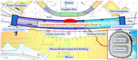
Figure 1.
Gongbei Tunnel’s concealed excavation portion.
2.1. Geological Conditions
The tunnel buried excavation portion, as illustrated in Figure 2, is in the transition zone between the continental edge’s shallow sea and the coastal alluvial plain. The sedimentary environment is relatively complicated, and there are geological changes between the tunnel’s left and right sides. The soil types in the formation, according to the exploration report, mostly comprise artificial backfill soil, silt and muddy soil, clay and silty clay, sandy gravel, weathered granite, etc., and their characteristics are shown in Table 1.
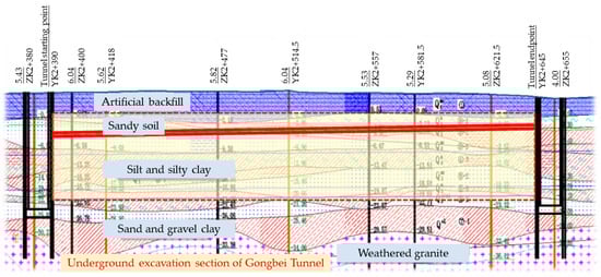
Figure 2.
Characteristics of stratum conditions in concealed excavation section.

Table 1.
Soil layer characteristics in concealed excavation section.
The surface layer is primarily composed of soft soil layers such as silt and muddy soil, which have the characteristics of wide distribution, large thickness, and significant local changes; high compressibility and sensitivity; and a humid climate with long and abundant rainfall, which forms a large supply of groundwater. The mucky soil in layers III-1, IV-3, and V-3, as well as the silt layer with greater humus, have engineering features such as high water content, high compressibility, and poor strength, which are detrimental to subterranean engineering excavation and stability.
2.2. Freezing Program for the FSPR Method
A horizontal zoning and vertical segmentation freezing method is used to avoid an excessive volume of frozen soil, according to the freezing construction organization design papers and pertinent requirements of the Gongbei Tunnel. As indicated in Figure 3, horizontal zoning freezing is mostly used to collaborate with underground excavation construction by separating the pipe curtain section into five zones: A, B1, B2, B3, and C. Vertical zoning freezing entails establishing two freezing stations on the east and west sides of the tunnel near the working shafts at both longitudinal ends, each with two systems (a refrigeration system and a limit system). To manage the opening and shutting of freezing tubes and limiting tubes, the pipe curtain is separated into three zones: freezing zone 1 (64 m), freezing zone 2 (128 m), and freezing zone 3 (64 m) from east to west.
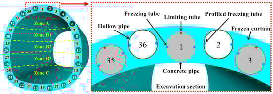
Figure 3.
Schematic presentation of FSPR applied in the Gongbei Tunnel.
Excessive frost heave can easily result in project risks since the tunnel passes through the customs port complex, near a significant number of subterranean pipelines and building piles, and is primarily surrounded by water-rich and soft soil layers. There are stringent criteria for mitigating the influence of ground frost heave, and the thickness of the frozen soil curtain should not be excessive. To achieve the above two requirements, careful real-time monitoring of the freezing temperature field is required during the building process:
- (1)
- Water sealing between jacked pipes should be safe with a minimum design value of frozen soil curtain thickness. The minimum thickness of the frozen soil curtain is planned to be 2 m, considering design characteristics such as pipe diameter, average separation between neighboring pipes, and misalignment angle;
- (2)
- The maximum design value of frozen soil curtain thickness cannot induce severe frost heave surface deformation. Because of the proportional relationship between the volume of frozen soil and the amount of surface frost heave, if the thickness of the frozen soil curtain is too thick, it will cause damage or even destruction to adjacent buildings (structures) and surrounding pipelines, affecting Gongbei Customs’ daily operations. The design thickness of the frozen soil curtain in the upper part of the tunnel (Zones A and B1) does not exceed 2.3 m, and the design thickness of the frozen soil curtain in the middle and lower parts of the tunnel (Zone B2C) does not exceed 2.6 m, according to the “Preliminary Research Report on Frost Heave Deformation during the Construction of the Gongbei Tunnel with the FSPR Method” and combined with relevant freezing engineering experience.
During the freezing phase, pick the freezing tube opening sequence and keep the temperature between −25 °C and −30 °C. Determine if the thickness of the frozen soil curtain matches the design criteria based on real-time data monitoring findings of temperature measurement locations in the soil layer. When the thickness of the frozen soil curtain approaches the minimum design value, the refrigeration system’s operating parameters should be modified promptly to prevent excessive development of the frozen soil curtain and to guarantee that its maximum thickness is between 2.3 m and 2.6 m.
3. Coupling Mathematical Model for Tunnel Freezing–Frost Heave
3.1. Mathematical Model for the Freezing Temperature Field
The transient heat conduction issue with phase transition includes the fluctuation of the freezing temperature field in the horizontal freezing tunnel [28,29]. Based on heat transfer and permafrost theories, and assuming that the temperature gradient of the low-temperature refrigerant in the freezing tube along the longitudinal direction (length direction) of the tunnel is approximately zero during the freezing process [30,31], the two-dimensional heat balance control differential equation of the freezing temperature field can be expressed as follows:
where
- —
Assuming that the soil’s freezing and melting temperatures are Td and Tr, respectively, and that no phase transition occurs when the soil temperature T < Td or T > Tr, the phase transition latent heat of water in ΩL = [Td, Tr] in Equation (1) can be derived and transformed into the phase transition latent heat of water-bearing soil, namely:
where
The differential equation for managing the heat balance of permafrost in the phase transition zone ΩL = [Td, Tr] can be found by substituting the derivation of Equation (2) into Equation (1):
By linear interpolating according to the temperature interval, the mass volume-specific heat CL and thermal conductivity λL in Equation (3) can be obtained:
where
The two-dimensional heat balance control differential equation of the freezing temperature field may be consistently stated by synthesizing Equations (1)–(5):
Equation (6)’s initial temperature requirement:
where T0 is the initial temperature of the soil, and a uniform temperature distribution is assumed. The temperature field in Equations (3)–(8) must meet continuity and energy conservation constraints at the phase transition boundary, i.e., at the frozen front S(t), namely:
where n is the phase transition boundary’s normal vector.
Because the freezing tube is significantly smaller than the tunnel and stratum, it may be treated as a single low-temperature point source, and the boundary conditions at the freezing tube are as follows:
where
The boundary conditions for soil at an infinite distance from the tunnel section:
When considering the heat exchange between the surface and the surrounding atmosphere, the surface may be seen as a convective heat transfer boundary, namely:
where
The preceding two-dimensional heat balance control differential equation, as well as its initial and boundary conditions, provide a mathematical description of the stratum’s transient freezing temperature field.
3.2. Coupling Mathematical Model for Freezing–Frost Heave
Thermal elastic–plastic analysis is performed with the features of the frozen soil curtain in mind [32,33]. Assuming frozen soil is an isotropic linear elastic material, its total strain {ε} may be thought of as a combination of elastic strain increment {ε}e induced by load and instantaneous bulk strain increment {ε}v caused by temperature change [34,35], namely:
The elastic strain increment {ε}e can be expressed:
where [D] is the elastic matrix, and its expression is as follows:
The thermal strain component produced by temperature change may be described in the local coordinate system as follows:
Hooke’s elastic theorem states that the total strain component of frozen soil in the local coordinate system is expressed as follows:
For the planar strain issue, with ε13 = ε23 = ε33 = 0, it can be obtained that:
The formula for the total strain of frozen soil in the local coordinate system is found by inserting Equation (18) into Equation (17):
The stress field equilibrium equation in the global coordinate system for the planar strain issue is as follows:
where γ is the soil gravity, and the geometric equation is
The displacement boundary conditions:
Given that mechanical properties of frozen soil—such as elastic modulus E and Poisson’s ratio μ—fluctuate with temperature, the thermodynamic coupling constitutive equation can be found by rewriting Equation (19):
According to the incremental theory [36,37,38], the stress–strain relationship for the assumed isotropic elastic–plastic unfrozen soil is as follows [39]:
where [D]ep is the elastic–plastic matrix and [D]p is the plastic matrix. And, there is
where F represents the yield function, P represents the plastic potential function, and A represents the hardening function. The coupling mathematical model of frost heave comprises Equations (6), (20) and (24).
4. Establishment of Finite Element Model
4.1. Numerical Calculation Model
Due to the tunnel’s complicated construction and geological circumstances, one of the cross-sections and its surrounding strata were chosen as the numerical computation object, as illustrated in Figure 4. The model has an overall dimension of 120 m × 60 m, and the geological condition has been simplified and separated into seven levels from the surface down. To assure the convergence and correctness of the calculation results, a planar triangular element was utilized for mesh division, and mesh refinement was performed in the pipe curtain area. The computation model has 215,091 elements, with an average element quality of 0.8264. For coupling, the calculation module employs the Solid Mechanics module and the Porous Medium Heat Transfer module [40,41].
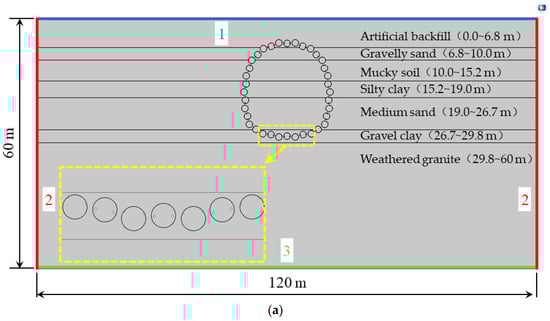
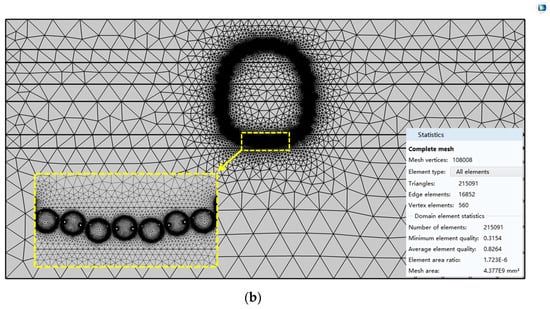
Figure 4.
Numerical calculation model: (a) Model size and soil layer distribution; (b) Computational domain grid.
4.2. Selection of Model Materials and Parameters
The yield criteria are based on the Drucker–Prager criterion, which assumes that all soil layers are ideal elastic–plastic constitutive models. Each soil layer’s material properties are established using the “Test Report of Physical and Mechanical Parameters of Artificial Frozen Soil at Gongbei Port on the Zhuhai side of the Hong Kong-Zhuhai-Macao Bridge”. The thermophysical parameters are listed in Table 2. Table 3 shows the mechanical properties of frozen soil, where the elastic modulus E of frozen soil is calculated using the interpolation procedure in the table, the freezing temperature T (°C) is negative, and the jacked pipe and concrete are considered elastic materials.
Table 2.
Thermophysical parameters of soil layer materials.
Table 3.
Mechanical parameters of materials.
4.3. Boundary Conditions and Calculation Assumptions
- (1)
- As shown in Figure 5, set the initial temperature of all soil layers to 20 °C, and the cooling plans for the circular freezing tubes in the concrete pipe and the profiled freezing tubes in the hollow pipe shall be taken based on their corresponding freezing system temperatures. Based on the engineering ambient temperature, the surface boundary (boundary 1) is set as a convective heat transfer boundary, while the borders on both sides (boundaries 2 and 3) and the bottom (boundary 4) are set as adiabatic, as shown in Figure 4a;
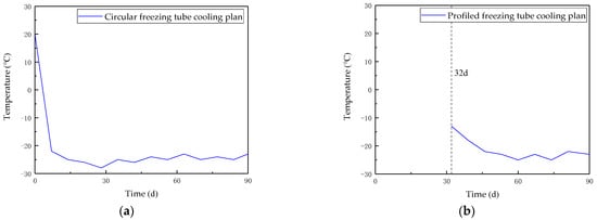 Figure 5. Cooling plan for two types of freezing tubes: (a) Circular freezing tubes; (b) Profiled freezing tubes.
 - (2)
- Without considering the surface load, the surface boundary (boundary 1) is regarded as a free boundary. Roller support is installed on both sides (boundaries 2 and 3), and only horizontal displacement is restricted. To restrict horizontal and vertical movement, fixed constraints are established at the bottom (boundary 4);
- (3)
- Assuming that the thermal resistance between different soil layers is zero, and ignoring the effect of soil moisture migration on the freezing process. The freezing point of all soil layers is uniformly set at −1.5 °C for the convenience of studying the size and shape of the frozen soil curtain.
To begin, an initial geostress field equilibrium analysis is performed to eliminate the initial vertical displacement of soil caused by gravity stress. Second, before the frost heave analysis, the model is subjected to volume force (soil gravity) and corresponding displacement boundary conditions to analyze the internal stress field of the soil at this time, and the data are derived and applied to the subsequent frost heave analysis model as the initial stress field of the soil. The soil maintains its equilibrium state without initial displacement due to the combined action of the initial stress field and the external volume force (gravity field), i.e., the initial vertical displacement of the soil is eliminated.
5. Analysis and Discussion of Calculation Results
5.1. Formation Law of Frozen Soil Curtain
Figure 6 depicts the cloud map of the temperature field distribution throughout the freezing phase. To study the changing features of the frozen soil curtain, the soil layer region around the 6# hollow pipe and 7# concrete pipe were intercepted. The frozen soil boundary (−1.5 °C) is denoted by the black line in each illustration.
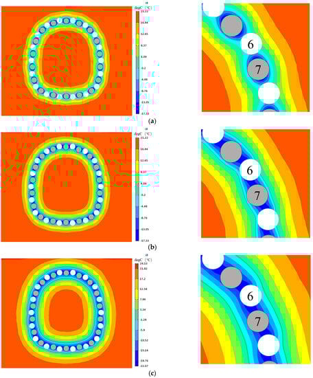
Figure 6.
Temperature field distribution during freezing phase: (a) 32 days; (b) 45 days; (c) 90 days.
According to the cooling plan, only the circular freezing tubes in the concrete pipe were opened in the first 32 days, as shown in Figure 6a. As the freezing time progresses, frozen soil forms near the circular freezing tubes at the two waist positions of each concrete pipe, and its range gradually expands from the pipe to the inside and outside of the pipe curtain. On day 32, the soil temperature in the pipe curtain area significantly decreased, particularly around the concrete pipes. The frozen soil curtain region has begun to “wrap” the concrete pipe and “overlap” with the neighboring hollow pipe but its size and temperature have not yet met the design requirements.
The soil temperature in the pipe curtain region rapidly decreased after the opening of the profiled freezing tubes in the hollow pipe from day 32 to day 45, and the distribution of the frozen soil curtain exhibited substantial changes compared to previously, as shown in Figure 6b. A frozen soil curtain of varying thickness has formed around the concrete pipes, with an average thickness range of 1.80 m to 1.87 m; the part of the hollow pipe located on the inner side of the pipe curtain has also been “wrapped” by the frozen soil; while a small portion on the outside has not been “wrapped”, the inner frozen soil curtain is developing faster than the outer side. The frozen soil between neighboring pipes also develops quite quickly, with an average thickness range of 1.82 m to 1.91 m and a temperature range of −0.2 °C to −17.3 °C.
After the frozen soil curtain has completely “wrapped” the hollow pipe, the frozen soil range on the inner and outer sides of the pipe curtain continues to expand but at a slower rate, and the temperature of the frozen soil between the adjacent pipes decreases further. When frozen for 90 days, the development of the frozen soil curtain begins to stabilize, as shown in Figure 6c. The average thickness increased somewhat, ranging from 2.32 m to 2.58 m, and the temperature range of the frozen soil between pipes is −7.2 °C to −22.1 °C, meeting the freezing design requirements.
The interface and axial plane between 6# hollow pipe and 7# concrete pipe were chosen as research subjects to explore the spatiotemporal impacts of temperature variations in frozen soil between adjacent pipes, as illustrated in Figure 7a. The distance between interface points was 0.4 m, while the distance between axial plane points was 0.09 m.
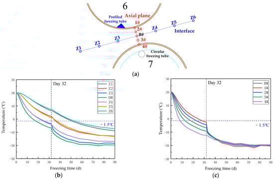
Figure 7.
Analysis of temporal and spatial variation of frozen soil temperature between jacked pipes: (a) Schematic diagram of measuring points; (b) Temperature–time curve of interface measurement points; (c) Temperature–time curve of axial plane measurement points.
Figure 7b depicts the temperature–time curves for each point on the interface. Because of the varying distances from point 0#, each curve shows “layering” and “symmetry” features from 0 d to 32 d. The average cooling rate at point 0# is −0.83 °C/d; the average cooling rates of Z3 and Z4, Z2 and Z5, and Z1 and Z6 are −0.74 °C/d, −0.57 °C/d, and −0.41 °C/d, respectively. When the profiled freezing tube in the hollow pipe was opened for operation after 32 days, all curves revealed a dramatic change in curvature, indicating that the cooling rate at each location had been increased once again. Simultaneously, because the position of the profiled freezing tube is closer to the inner side of the pipe curtain, the curve of Z3 is substantially lower than that of Z4. The average cooling rates of 0#, Z3, and Z4 were −0.76 °C/d, −0.85 °C/d, and −0.6 °C/d, respectively, during 32 to 45 days, indicating that the profiled freezing tube has a strong freezing strengthening effect. The total temperature range of the interface was −7.3 °C~−19.7 °C after 90 days, and the temperature on the inner side of the pipe curtain was slightly lower than that on the outer side. The overall distribution was relatively uniform.
Figure 7c depicts the temperature–time curve for each point on the axial plane. The difference from the interface temperature distribution with the average cooling rate in 32 d~45 d is that the closer the point is to the 6# hollow pipe, the higher the average cooling rate. The cooling rates of 1#, 2#, 0#, 3#, and 4# are −1.17 °C/d, −0.97 °C/d, −0.76 °C/d, −0.56 °C/d, and −0.34 °C/d, respectively. The temperature curve variations at each location eventually tend to be horizontal and overlap after 70 days, showing that the temperature differential between adjacent jacked pipes steadily narrows. By 90 days, the temperature at each location is nearly identical, with an overall value of −19.9 °C.
According to the above analysis, the process of forming a frozen soil curtain and the distribution features of the freezing temperature field are directly connected to the layout and opening time sequence of the two types of freezing tubes in hollow and concrete pipes. The results of the calculations demonstrate that the thickness and temperature distribution of the frozen soil curtain can match the design requirements, and that it has high water sealing and safety performance, producing ideal support conditions for future tunnel section excavation.
5.2. Distribution Law of Stratum Frost Heave Displacement
The size of the frozen soil curtain grows larger with time, causing vertical and horizontal displacement of the stratum due to frost heave. Figure 8 depicts the distribution features of the vertical frost heave displacement field. The highest vertical frost heave displacement at 32 d is 26.08 mm. The formation of the frozen soil curtain is relatively slow during the first 32 days because only the circular freezing tube inside the concrete pipe is opened for freezing; after 32 days, the formation rate accelerates due to the opening of the profiled freezing tube to strengthen the freezing. The maximum displacement is 75.5 mm after 45 days and 133.69 mm after 70 days. Following that, the size of the frozen soil curtain changes insignificantly, with a maximum displacement of 167.49 mm at 90 days.
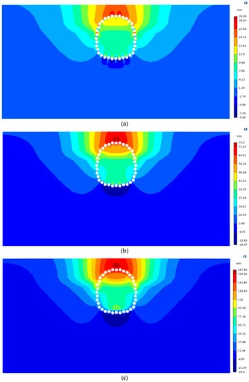
Figure 8.
Vertical frost heave displacement distribution of stratum: (a) 32 days; (b) 45 days; (c) 90 days.
Because of the model’s symmetry, the vertical frost heave displacement field is horizontally symmetrical in general, and its value increases with the time of freezing. The maximum positive value of vertical displacement always appears near the top of the pipe curtain, related to the tunnel’s shallow buried depth, the thin covering soil layer, and the comparatively large volume of frozen soil. The vertical frost heave displacement decreases as soil depth increases, indicating that the larger effective stress of deep soil partially offsets the frost heave force, which has a limiting effect on frost heave deformation until the vertical displacement at the bottom of the pipe curtain shows a small negative value. The vertical frost heave displacement in the tunnel excavation segment is quite minor due to the overall stiffness of the pipe curtain.
As shown in Figure 9, the horizontal frost heave displacement field, like the vertical frost heave displacement field, changes slightly within 0–32 days, with a maximum value of 20.64 mm at 32 d. It increased rapidly from 32 d to 70 d, with maximum values of 39.9 mm and 56.8 mm at 45 d and 70 d, respectively. The development then slows in 70 to 90 days, reaching a maximum of 72.3 mm at 90 days.
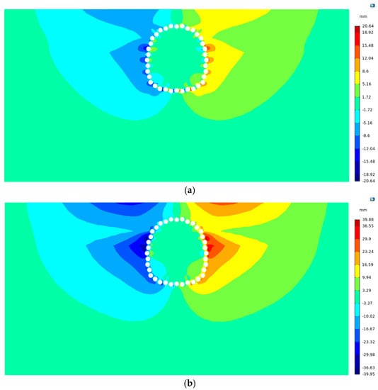
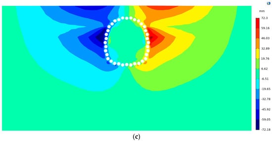
Figure 9.
Horizontal frost heave displacement distribution of stratum: (a) 32 days; (b) 45 days; (c) 90 days.
Overall, the stratum’s horizontal frost heave displacement field has a horizontally antisymmetric distribution, and its absolute magnitude increases with the duration of continuous freezing. In addition to the ground surface, areas with high displacement values are distributed beyond the pipe curtain’s waist, where there is primarily a silty clay layer with high water content and a high frost heave rate, causing significant deformation as the thickness of the frozen soil curtain increases during the freezing process. The horizontal frost heave displacement is quite minor in the tunnel excavation segment.
5.3. Distribution Law of Ground Surface Frost Heave Displacement
Figure 10a depicts the ground surface’s vertical frost heave displacement distribution curve. The tunnel centerline (x = 0 m) serves as the symmetry axis for all the curves. The vertical displacement of each point rises with freezing duration, and the effect is particularly noticeable in the −30 m ≤ x ≤ 30 m. range. The highest vertical uplift value of the surface at any moment in time is found at the center line, and the farther the location is from the center line, the lower the value is and ultimately approaches zero.
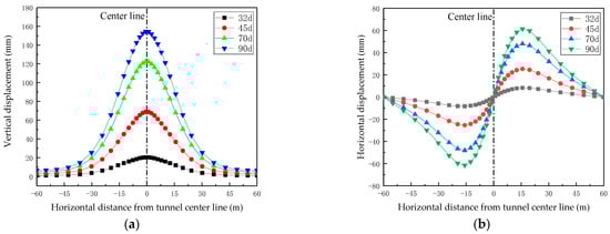
Figure 10.
Frost heave displacement distribution curve of ground surface: (a) Vertical displacement curve; (b) Horizontal displacement curve.
Within 32 days to 70 days, there is a considerable rise, with maximum values of 68.96 mm and 122.4 mm at 45 and 70 days, respectively, and 10.71 mm and 19.38 mm at ±30 m from the centerline. From 70 d to 90 d, the range of variation was rather minimal, with a maximum value of 155.67 mm at 90 d and 25.36 mm at 30 ±m from the center line.
The ground surface’s horizontal frost heave displacement distribution curve is shown in Figure 10b, with the tunnel centerline (x = 0 m) as the axis of symmetry—indicating an anti-symmetric distribution—and the displacement at the centerline being zero at all times. The displacement values on both sides of the centerline first gradually increase with distance, reaching the extreme value at x = ±15.74 m, and then gradually decreasing to zero.
The horizontal displacement of the ground surface changes relatively little from 0 d to 32 d, with an average increase of 0.26 mm/d and an extreme value of 8.17 mm at 32 d. It quickly increases from 32 to 45 days, with an average rate of 1.25 mm/d and an extreme value of 24.47 mm at 45 days. It slows down from 45 d to 70 d, with an average rate of 0.88 mm/d and an extreme value of 46.44 mm at 70 d; from 70 d to 90 d, with an average rate of 0.66 mm/d and an extreme value of 59.63 mm at 90 d.
Comparing the numerical calculation results of vertical frost heave displacement at the surface midpoint of the selected model cross-section with the field-measured values, as shown in Figure 11, the variation patterns of the two are basically consistent, with some points having deviations less than 15 mm. The displacement value fluctuates relatively little from 0 d to 10 d, with an average increase rate of 0.07 mm/d. The displacement value varied relatively little from 0 to 10 d, with an average growth rate of 0.07 mm/d, then gradually increased to 0.93 mm/d from 10 d to 32 d. The displacement curve changes significantly from 32 d to 45 d, with an average increase rate of 3.47 mm/d, which then decreases to 2.14 mm/d from 45 d to 70 d, and further decreases to 1.54 mm/d from 70 d to 90 d. The numerical calculation result was 155.67 mm at 90 d, whereas the measured datum was 157.41 mm, showing that the calculation results are acceptable.
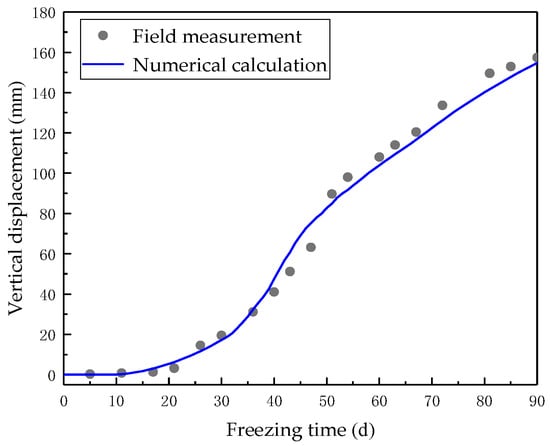
Figure 11.
Comparison of simulated and measured vertical displacement of ground surface midpoint.
The findings of the foregoing study show that the distribution and change of frost heave displacement during the freezing period are directly connected to the engineering geological circumstances, freezing scheme, forming process of frozen soil curtain, and pipe curtain structure.
6. Conclusions
- (1)
- The formation of the frozen curtain during the freezing process is mostly dependent on two types of freezing tubes to freeze the soil between the jacked pipes and fulfill the objective of sealing water. At 90 days, the thickness of the frozen soil curtain varies from 2.32 m to 2.58 m, and the lower and more homogeneous frozen soil temperature between adjacent pipes ensures that its strength fulfills the water-sealing safety requirements;
- (2)
- The frost heave displacement distribution and fluctuation throughout the freezing phase are highly connected to geological conditions, freezing scheme, frozen soil curtain development, and pipe curtain structure. The ground surface’s vertical frost heave displacement curve is normally distributed with the tunnel centerline (x = 0 m) as the symmetry axis, and the change is more noticeable in the range of −30 m ≤ x ≤ 30 m; the maximum value at any time is located at the centerline, which is 155.67 mm at 90 d. The horizontal displacement at the ground surface’s center line is always zero, while the values on both sides of the centerline progressively rise with distance, reaching an extreme value at x = 15.74 m, 59.63 mm at 90 d;
- (3)
- In this study, the geological conditions, temperature gradient, and numerical model are appropriately simplified, and the calculation object is the two-dimensional cross-section of the tunnel during the freezing phase. Although the calculation results are in good agreement with the measured data and have good guiding value for engineering construction, it is still a topic worth further research on how to more accurately reflect complex actual working conditions and focus on establishing more precise large-scale numerical models considering subsequent construction phases, such as tunnel excavation, support structure construction, and ground thawing settlement.
Author Contributions
Conceptualization, Y.D.; methodology, Y.D.; software, Y.D. and W.L.; validation, Y.D. and C.R.; writing—original draft preparation, Y.D.; writing—review and editing, Y.D. and W.L. All authors have read and agreed to the published version of the manuscript.
Funding
This research was funded by the Scientific Research Foundation for High-level Talents of Anhui University of Science and Technology, grant number 2022yjrc55; and the National Natural Science Foundation of China, grant number 51878005.
Data Availability Statement
The datasets generated and analyzed during the current study are available from the corresponding author upon reasonable request.
Conflicts of Interest
The authors declare no conflict of interest.
References
- National Bureau of Statistics. China Statistical Yearbook; China Statistical Press: Beijing, China, 2022; pp. 2–6. (In Chinese)
- He, X.L.; Li, J.Y. Demographic Structure, Consumption Structure of Residents and Industrial Upgrading. Reg. Econ. Rev. 2023, 63, 90–100. [Google Scholar] [CrossRef]
- Zucca, M.; Valente, M. On the limitations of decoupled approach for the seismic behaviour evaluation of shallow multi-propped underground structures embedded in granular soils. Eng. Struct. 2020, 211, 110497. [Google Scholar] [CrossRef]
- Xiong, Z.M.; Lu, H.; Wang, M.Y.; Qian, Q.H.; Rong, X.L. Research progress on safety risk management for large scale geotechnical engineering construction in China. Rock Soil Mech. 2018, 39, 3703–3716. [Google Scholar] [CrossRef]
- Ma, P.; Shimada, H.; Sasaoka, T.; Hamanaka, A.; Dintwe, T.K.M.; Pan, D. Investigation on the Performance of Pipe Roof Method Adjacent to the Underground Construction. Geotech. Geol. Eng. 2021, 39, 4677–4687. [Google Scholar] [CrossRef]
- Zhu, Y.F.; Guo, Y.; Pan, W.Q.; Zhao, X.P. Application of Pipe-roofing Method with Various Section Types in Metro Construction of Guiqiao Road Station at Saturated Soft Soil Area. Tunn. Constr. 2020, 40, 552–561. [Google Scholar]
- Zucca, M.; Crespi, P.; Tropeano, G.; Marco, S. On the Influence of Shallow Underground Structures in the Evaluation of the Seismic Signals. Ing. Sismica 2021, 38, 23–35. [Google Scholar]
- Hemerijckx, I.E. Tubular thrust jacking for underground roof construction on the Antwerp metro. Int. J. Rock Mech. Min. Sci. Geomech. Abstr. 1983, 20, 27–30. [Google Scholar] [CrossRef]
- Liao, H.J.; Cheng, M. Construction of a piperoofed underpass below groundwater table. Proc. Ice Geotech. Eng. 1996, 119, 202–210. [Google Scholar] [CrossRef]
- Ge, J.K. Study on tunnel construction scheme by pipe-roofing in saturated soft strata. In Proceedings of the Geo-Shanghai, Shanghai, China, 10–11 November 2004. [Google Scholar]
- Kang, C.G. Discussion on Tube Curtain Slurry-balanced Pipe-jacking Construction Technology of Beijing Subway Line 4. J. Water Resour. Archit. Eng. 2012, 10, 91–94. [Google Scholar] [CrossRef]
- Li, Y.S.; Zhang, K.N.; Huang, C.B.; Li, Z.; Deng, M.-L. Analysis of surface subsidence of tunnel built by pipe-roof pre-construction method. Rock Soil Mech. 2011, 32, 3701–3707. [Google Scholar] [CrossRef]
- Wang, X.D. Design and Construction of the Gaoqiao Tunnel on the Zhengzhou-Xi’an Passenger Dedicated Line Passing Under the Existing Railway. Mod. Tunn. Technol. 2012, 49, 132–137. [Google Scholar] [CrossRef]
- Gou, M.Z. Key Technology for Design and Construction of Highway Tunnel Crossing underneath Operating Railway Lines with Small Clearance. Tunn. Constr. 2013, 33, 59–64. [Google Scholar]
- Xiao, D.D. Study on the Tunnel Structural Design and Construction Mechanics Effect of the New Tubular Roof Method on the TaiYuan Railway Station. Master’s Thesis, Shijiazhuang Tiedao University, Shijiazhuang, China, 2018. [Google Scholar]
- Li, Y.L.; Zhang, Y.H.; Li, W.Q. Research and Application of Pipe Roofing Method in Soft Soil. Chin. J. Undergr. Space Eng. 2011, 7, 962–967. [Google Scholar] [CrossRef]
- Artem, V.; Jianzhong, X.; Zhuye, H.; Haojie, Z. Analyses of Artificial Ground Freezing with Carbon Dioxygen to Protect Foundation Pit from High Ground Velocity Water Flow. J. Eng. Archit. 2019, 7, 2334–2994. [Google Scholar] [CrossRef]
- Russo, G.; Corbo, A.; Cavuoto, F.; Autuori, S. Artificial Ground Freezing to Excavate a Tunnel in sandy Soil. Measurements and Back Analysis. Tunn. Undergr. Space Technol. 2015, 50, 226–238. [Google Scholar] [CrossRef]
- Hu, X.D.; Fang, T. Numerical Simulation of Temperature Field at the Active Freeze Period in Tunnel Construction Using Freeze-Sealing Pipe Roof Method. In Proceedings of the Geo-Shanghai, Tunneling and Underground Construction, Shanghai, China, 26–28 May 2014; pp. 731–741. [Google Scholar] [CrossRef]
- Hu, X.D.; Ren, H.; Chen, J.; Cheng, Y. Model Test Study of the Active Freezing Scheme for the Combined Pipe-Roof and Freezing Method. Mod. Tunn. Technol. 2014, 51, 92–98. [Google Scholar] [CrossRef]
- Ren, H.; Hu, X.D.; Chen, J. Study on Freezing Effect and Operation of Profiled Enhancing Freezing tube in Freeze sealing Pipe Roof. Tunn. Constr. 2015, 35, 1169–1175. [Google Scholar] [CrossRef]
- Kang, Y.S.; Liu, Q.S.; Yong, C.; Liu, X. Combined freeze-sealing and New Tubular Roof construction methods for seaside urban tunnel in soft ground. Tunn. Undergr. Space Technol. Inc. Trenchless Technol. Res. 2016, 58, 1–10. [Google Scholar] [CrossRef]
- Hu, X.D.; Deng, S.J.; Wang, Y. Mechanical tests on bearing capacity of steel pipe-frozen soil composite structure applied in Gongbei Tunnel. Chin. J. Geotech. Eng. 2018, 40, 1481–1490. [Google Scholar] [CrossRef]
- Zhang, D.M.; Pang, J.; Ren, H.; Han, L. Observed deformation behavior of Gongbei Tunnel of Hong Kong-Zhuhai-Macao Bridge during construction. Chin. J. Geotech. Eng. 2020, 42, 1632–1641. [Google Scholar] [CrossRef]
- Duan, Y.; Rong, C.; Cheng, H.; Cai, H.; Long, W. Freezing Temperature Field of FSPR under Different Pipe Configurations: A Case Study in Gongbei Tunnel, China. Adv. Civ. Eng. 2021, 2021, 9958165. [Google Scholar] [CrossRef]
- Duan, Y.; Rong, C.; Huang, X.; Long, W. An Analytical Solution to Steady-State Temperature Field in the FSPR Method Considering Different Soil Freezing Points. Appl. Sci. 2022, 12, 11576. [Google Scholar] [CrossRef]
- Duan, Y.; Rong, C.; Cai, H.; Long, W. Experimental research on mechanical properties of “jacked pipe-frozen soil” composite structure in freeze-sealing pipe roof tunnel. Coal Geol. Explor. 2022, 50, 159–169. [Google Scholar] [CrossRef]
- Zhang, X.; Lai, Y.; Yu, W.; Zhang, S. Nonlinear analysis for the three-dimensional temperature fields in cold region tunnels. China Civ. Eng. J. 2003, 35, 207–219. [Google Scholar] [CrossRef]
- Alzoubi, M.A.; Xu, M.; Hassani, F.P.; Poncet, S.; Sasmito, A.P. Artificial ground freezing: A review of thermal and hydraulic aspects. Tunn. Undergr. Space Technol. 2020, 104, 103534. [Google Scholar] [CrossRef]
- Zhang, X.; Lai, Y.; Yu, W.; Zhang, S. Numerical analysis for the three-dimension temperature fields in cold region tunnels. J. China Railw. Soc. 2003, 25, 84–90. [Google Scholar] [CrossRef]
- Lai, Y.M.; Wu, Z.W.; Zhu, Y.L.; Zhu, L.N. Nonlinear analysis for the coupled problem of temperature, seepage and stress fields in cold-region tunnels. Tunn. Undergr. Space Technol. 1998, 13, 435–440. [Google Scholar] [CrossRef]
- Zhao, Y.; Liang, C. Coupling Analysis of temperature and elastic-plastic stress field of frozen shaft walling. In Proceedings of the 3rd Rock Mechanics Academic Conference, Beijing, China, 20–23 August 1985; pp. 1–20. (In Chinese). [Google Scholar]
- Bekele, Y.W.; Kyokawa, H.; Kvarving, A.M.; Kvamsdal, T.; Nordal, S. Isogeometric analysis of THM coupled processes in ground freezing. Comput. Geotech. 2017, 88, 129–145. [Google Scholar] [CrossRef]
- Chen, H.; Zang, H. Quasi-coupling numeric analysis of frost heave effect of horizontal freezing in artificial ground. Chin. J. Geotech. Eng. 2003, 25, 87–90. [Google Scholar] [CrossRef]
- Wu, G.X.; Liu, Y.M.; Liu, X.; Duan, A.M. Numerical method of phase-change field of temperature coupled with moisture, stress in frozen soil. J. Tongji Univ. 2005, 33, 1281–1285. [Google Scholar] [CrossRef]
- Qiu, J.; Guo, N.; Liu, Z. Solution on freezing temperature stress during underground construction by freezing method. J. China Railw. Soc. 2000, 22, 78–83. [Google Scholar]
- Wang, T.; Hu, C.; Li, N. Stress-strain numerical model for frozen soil subgrade. Chin. J. Geotech. Eng. 2002, 24, 193–197. [Google Scholar] [CrossRef]
- Wang, Z.; Ma, W.; Sheng, Y.; Wu, Z. A Progressive Yield Criteria on Creep of Frozen Soil. J. Glaciol. Geocryol. 1999, 2, 61–67. [Google Scholar]
- Lai, Y.; Wu, Z.; Zhu, Y. Nonlinear analyses for the couple problem of temperature, seepage and stress fields in cold region tunnels. Chin. J. Geotech. Eng. 1999, 21, 529–533. [Google Scholar]
- COMSOL Multiphysics Application Programming Guide. 2022. Available online: http://cdn.comsol.com/doc/6.1.0.357/ApplicationProgrammingGuide.zh_CN.pdf (accessed on 1 June 2022).
- Panteleev, I.; Kostina, A.; Plekhov, O.A. Numerical Simulation of Artificial Ground Freezing in a Fluid-Saturated Rock Mass with Account for Filtration and Mechanical Processes. Cold Arid Reg. 2017, 9, 363–377. [Google Scholar]
Disclaimer/Publisher’s Note: The statements, opinions and data contained in all publications are solely those of the individual author(s) and contributor(s) and not of MDPI and/or the editor(s). MDPI and/or the editor(s) disclaim responsibility for any injury to people or property resulting from any ideas, methods, instructions or products referred to in the content. |
© 2023 by the authors. Licensee MDPI, Basel, Switzerland. This article is an open access article distributed under the terms and conditions of the Creative Commons Attribution (CC BY) license (https://creativecommons.org/licenses/by/4.0/).