Abstract
The problem of sparse-view computed tomography (SVCT) reconstruction has become a popular research issue because of its significant capacity for radiation dose reduction. However, the reconstructed images often contain serious artifacts and noise from under-sampled projection data. Although the good results achieved by the prior image constrained compressed sensing (PICCS) method, there may be some unsatisfactory results in the reconstructed images because of the image gradient L1-norm used in the original PICCS model, which leads to the image suffering from step artifacts and over-smoothing of the edge as a result. To address the above-mentioned problem, this paper proposes a novel improved PICCS algorithm (NPICCS) for SVCT reconstruction. The proposed algorithm utilizes the advantages of PICCS, which could recover more details. Moreover, the algorithm introduces the L0-norm of image gradient regularization into the framework, which overcomes the disadvantage of conventional PICCS, and enhances the capability to retain edge and fine image detail. The split Bregman method has been used to resolve the proposed mathematical model. To verify the effectiveness of the proposed method, a large number of experiments with different angles are conducted. Final experimental results show that the proposed algorithm has advantages in edge preservation, noise suppression, and image detail recovery.
1. Introduction
In recent years, X-ray computed tomography (CT) has been able to capture images of internal organ tissues and structures by a non-destructive technique, which has been successfully used in various fields such as archaeology, medical diagnosis, and industrial inspection [1,2]. But there has been growing concern that the human body will absorb some X-rays, leading to a risk of cancer [3,4]. To avoid excessive radiation doses, the well-known ALARA (as low as reasonably achievable) principle is extensively applied in clinical practice. Commonly, there are two methods to reduce the radiation dose, for example, reducing the detector unit X-ray flux and decreasing the scanned views [5,6,7,8]. However, reducing the radiation dose and the scanned views usually cause high noise and artifacts in the reconstructed images by conventional filtered back projection (FBP) [9]. Therefore, how to reconstruct a satisfactory image from noisy projection data or under-sampled projection data has become a hot research issue. This work focuses on the under-sampled projection data case.
In order to obtain finely detailed reconstructed images from under-sampled projection data, researchers have proposed some iterative reconstruction methods. Typical iterative reconstruction algorithms such as the algebraic reconstruction technique (ART) [10], the simultaneous algebraic reconstruction technique (SART) [11], and expectation maximization (EM) [12] combined with prior regularization constraint could improve image quality to a certain extent. Total variation (TV), as a simple and effective regularization, has been widely applied in the CT field [13,14]. But the disadvantage of TV is the assumption that the reconstructed image is constructed of piecewise constants [15], leading to serious staircase artifacts in the reconstructed image. Therefore, variant methods have been presented to improve the image quality. Tian et al. proposed an edge-preserving total variation (EPTV) method, which allocated different weights to penalize the pixels at the non-edge or edge position in the image [16]. Kim et al. developed a non-local total-variation (NLTV) minimization method, which combined with reweighted L1-norm to process image [17]. Liu et al. presented an adaptive-weighted total variation (AWTV) regularization, which considered the weights depending on the anisotropic edge properties between adjacent image voxels [18]. Niu et al. used a penalized weighted least-squares (PWLS) method with a total generalized variation (TGV), which showed the advantage in reconstruction accuracy [19]. Yu et al. presented a novel regularization combined constraint structural group sparsity with TV prior sparsity, which effectively suppressed the noise and artifacts [20]. Although the above-mentioned methods have advantages in suppressing staircase artifacts effects, they are still based on TV and may lose subtle details and blur the image edge. Later in the CT reconstruction field, dictionary learning (DL) was proposed and had demonstrated great potential. DL methods were firstly developed by Xu et al. [21] for low-dose CT (LDCT) image reconstruction via combining the PWLS method with regularization involving redundant pre-learned dictionaries. Dong et al. designed a new discriminative dictionary for both the reconstruction and segmentation, providing better results than common dictionary-based methods [22]. Gui et al. proposed an iterative reconstruction algorithm for LDCT images based on image block classification and dictionary learning to address the limitation that all image blocks are represented by the same dictionary, which greatly improved the image quality [23]. Wu et al. combined the L1-norm dictionary learning penalty with a statistical iterative reconstruction framework for LDCT image reconstruction, which accelerated the global convergence rate [24]. Zhi et al. designed a spatially structural two-dimensional dictionary and a motion-aware dictionary for four-dimensional CT reconstruction [25]. But most DL methods extract patches from the image and operate based on a patch, which causes concern that the image may render new patch aggregation artifacts at the patch boundary. Therefore, the convolutional sparse coding (CSC) method was presented and achieved better reconstruction results [26,27].
Different from the afore-mentioned methods, it is worth emphasizing that the quality of CT images will be improved if a prior image is introduced. Therefore, in 2010, Qi et al. proposed a method based on prior image constrained compressed sensing (PICCS), which reduced noise and radiation dose in breast cone beam CT imaging [28]. Szczykutowicz et al. designed a novel denoising method based on PICCS for dual energy CT [29]. Lee et al. presented an adaptive PICCS method to enhance 4D CBCT reconstruction image quality [30]. Essam A. Rashed et al. proposed a powerful statistical image reconstruction algorithm for CT for which prior information obtained from a probabilistic atlas is modeled for the CT image reconstruction [31]. Pascal Theriault Lauzier et al. applied the PICCS reconstruction method in the cardiac interventional setting, which solved the view angle under-sampling and projection data truncation problems, causing by cardiac gating and the small size of the detector [32]. Chen et al. proposed a sparse-view CT reconstruction method based on PICCS, which introduced a prior image to accurately reconstruct dynamic CT images from under-sampled projection datasets, and achieved good results [33,34]. Later, the methods based on PICCS were widely used in energy spectrum CT reconstruction, which greatly improved the quality of energy spectrum CT reconstruction [35,36,37,38]. However, most PICCS-based methods are based on TV sparse framework, and the gradient L1-norm may cause blurred edges and loss image details. Recently, the image gradient L0-norm has been extensively used in image restoration, image segmentation, and image smoothing [39,40,41]. It achieved better performance in sparse-view, limited-view, and LDCT reconstruction such as edge preservation, artifact reduction, and noise suppression [42,43]. The primary reason is that the image gradient L0-norm does not penalize large image gradient magnitudes, which may be more suitable for preserving image edge and reducing noise.
In this work, based on the pioneering research of PICCS, we propose a novel improved PICCS algorithm for SVCT reconstruction (NPICCS). Firstly, the algorithm continues to utilize the advantage of prior image constrained compressed sensing, which recovers more details. Moreover, by introducing the L0-norm of the image gradient regularization term into the algorithm framework, not only the edge information can be effectively preserved, but also noise can be greatly reduced.
The major contribution of this article is manifested in the following two aspects. Firstly, the innovative introduction of L0-norm regularization to the PICCS framework for SVCT reconstruction not only enhances the ability to preserve image details, but also reduces noise and artifacts in the images. Secondly, an effective split Bregman algorithm is employed to solve the NPICCS optimization model.
The remainder of the article is structured as follows. In Section 2, some relevant algorithm models and fundamental theory are briefly introduced. The method to solve the algorithm model is described in Section 3. Section 4 discusses and compares some representative experiments. In the last section, we present the conclusion and discussion.
2. Related Work
This section briefly reviews some relevant work, including mathematical models and fundamental theories related to PICCS for CT reconstruction and image gradient L0-norm minimization.
2.1. CT Reconstruction Based on PICCS
By using a reconstruction algorithm, CT reconstruction collects X-ray projection data recorded by the detector at different views to obtain the linear attenuation coefficient of the scanned object. In the sparse-view reconstruction, in order to suppress noise and artifacts in the reconstructed image and obtain a reasonable approximate solution, it is usually necessary to introduce a regularization term to optimize the model, and the specific optimization model can be expressed as follows:
A = {ai,j}∈RIxJ is a system matrix, I and J stand for the number of X-rays and image pixels, respectively. x represents the reconstructed image, in whose value is the X-ray’s linear attenuation coefficient. Y stands for the projection data. Hence, the core problem in CT reconstruction is commonly regarded as an inverse problem, which reconstructs the image x from A and Y. In practice, x can be calculated by addressing the least squares problem:
To solve the ill-posed inverse problem and acquire reasonable approximate solutions, especially for SVCT, appropriate regularization term should be introduced. For simplicity, the problem can be represented as follows:
The first and second term are data fidelity and a regularization term such as TV, TGV, and wavelet framework, etc., respectively. μ is a scale parameter, which balances the regularization term and data fidelity term. When a prior image is available, it could be appended to the second regularization term. Therefore, the PICCS image reconstruction is achieved by resolving the following minimization problem [34]:
where a is the empirical parameter and xprior is a prior image. TV denotes the image gradient L1-norm, which is expressed as follows:
where i and j stand for the pixel position of image. xi,j are the pixel values at the position.
2.2. Image Gradient L0-Norm Minimization
The successful application of the image gradient L0-norm in image processing has inspired scholars to start developing it for limited-view and SVCT reconstruction. The main principle of the image gradient L0-norm is to count the number of non-zero elements. The mathematical expression is denoted as follows:
where p (p = 1, 2, …, N1 × N2) represents the location of (n1, n2) in the image. The (ძix)p and (ძjx)p denote (x(n1,n2) − x(n1 − 1,n2)) and (x(n1,n2) − x(n1,n2 − 1)). Ψ is a counting operator, which can be defined as follows:
It could be observed from Equation (7) that the gradient L0-norm does not penalize the values with large gradients, which indicates that edge information and more small structures are more likely to be retained.
3. Method
3.1. Mathematical Model
Despite the good results achieved by the PICCS algorithm in CT reconstruction, there may be some unsatisfactory results in the reconstructed images because of the image gradient L1-norm used in the original PICCS model, which leads to the image suffering from step artifacts and over-smoothing of the edge as a result. In order to resolve the above-mentioned problem, it is necessary to introduce a new regularization constraint. Therefore, we incorporate the image gradient L0-norm to the original PICCS framework to enhance the ability of image edge preservation and artifacts reduction. The specific objective function is defined as follows:
where xprior is a prior image, which comes from a full-view projection with noise by the direct FBP reconstruction in this work.
3.2. Solution
For the above model, Equation (8) is a non-convex and NP-hard problem since it contains a gradient L0-norm. To resolve this problem efficiently, we first introduce two additional parameters c1 and c2; Equation (8) could be redefined as a constrained optimization problem as follows:
Then, the above problem can be converted into an unconstrained problem by utilizing the scaled augmented Lagrangian function [44], mathematical model as follows:
where m1 and m2 are auxiliary variables, and λ1and λ2 represent two Lagrangian multipliers. We utilize the split Bregman (SB) algorithm to divide Equation (10) into the following sub-problems:
Sub-problem 1:
Sub-problem 2:
Sub-problem 3:
Equation (11) can be resolved via the separable surrogate algorithm [45] as follows:
Because Equations (12) and (13) are similar, we only discuss the solution of (13). c2 is obtained by minimizing the L0-norm, which is not easily solved directly. So, we reference an approximate method in the literature [46] to solve it. Firstly, we introduce two auxiliary variables (u2k and v2k) in place of the x- and y- direction of c2, and Equation (13) can be transformed as follows:
where γ2 = 2 × (1 − a)/λ2 affects the ability of image edge retention. τ2 is utilized to trade off the proximity between (u2k, v2k) and (ძx(c2k), ძy(c2k)). Equation (17) has three parameters, and we still use the SB algorithm to compute. Equation (17) can be further converted into the two steps, as follows:
Step 1:
Step 2:
For Equation (18), the optimal condition is as follows:
where τ2 is adjusted in iterations automatically, which starts from small values of τ02, and each time it is multiplied by k2. The same process is used for τ1 associated with the Equation (12), where τ1, τ2, and τmax have fixed values of 2γ1, 2γ2, and 105, respectively. k1 and k2 are set to 1.4 and 1.2, which could provide a good trade-off between performance and efficiency.
To address the optimization Equation (19), we utilize a fast method in the reference [47] combining the diagonalized derivative operator and the Fourier transform convolution theorem. The solution of Equation (19) could be denoted as follows:
F and F* stand for Fourier transform and conjugate Fourier transform, respectively. In conclusion, the pseudocode is displayed in Algorithm 1.
| Algorithm 1: NPICCS |
| Input: a, γ1, γ2, τmax, k1, k2, Niter, xprior Initialize: x(0) = c1(0) = c2(0) = m1(0) = m2(0) = 0 for N < Niter Update x(n+1) by Equation (16); while (τ1 ≤ τmax) do Update {(u1k) r+1, (v1k) r+1} same as Equation (20); Update c1r+1 same as Equation (21); τ1 = k1τ1, r = r + 1 end while while (τ2 ≤ τmax) do Update {(u2k) r+1, (v2k) r+1} by Equation (20); Update c2r+1 by Equation (21); τ2 = k2τ2, r = r + 1 end while Update c(n+1): c1n+1 = c1r+1, c2n+1 = c2r+1; Update m1(n+1), m2(n+1) by Equations (14) and (15); n = n + 1 when satisfy the stopping condition, stop iterating end for output: reconstruction image x |
4. Experimental Results
In order to demonstrate the effectiveness and feasibility of our method, we conducted multiple experiments for two typical CT images—pelvic and abdomen images. This work utilized the algorithm in reference [48] to generate projection data. The size of the images is 256 × 256. From the X-ray source to the detector/scanned object, the distance is 80 cm and 40 cm, respectively. The number of detectors is 512, with a length of 41.3 cm. In practical applications, noise is unavoidable, so the projection data have added some degree of Poisson noise, the level of which can be changed via the incident photons number. We set the value as 106 in this experiment. Five algorithms were used for comparison: FBP, OS-SART, TV minimization, PICCS, and a guided image filter reconstruction based on TV and prior image (TVPI-G) [49]. The initial image was set to zero for all iterative algorithms. The maximum number of iterations was set to 500, and the iteration stops when the algorithm converges. RMSE, SSIM [50], and PSNR are calculated to analyze the image quality quantitatively.
4.1. Image Reconstruction Experiment of Pelvic Image
The first image reconstruction experiment is using a pelvic image to show the feasibility of our algorithm for SVCT reconstruction, as shown in Figure 1. We extracted 80, 64, and 48 views from a full scan and selected parameters empirically. The parameters are set as follows: a = 0.5, γ1 = 0.3, and γ2 = 0.08. Figure 2, Figure 3 and Figure 4 show the ground truth and reconstruction images via FBP, OS-SART, TV, PICCS, TVPI-G, and our method NPICCS. From these figures, it is evident that our algorithm outperforms the other methods in terms of recovering image structures and suppressing noise. Specifically, the FBP and OS-SART results (as shown in Figure 2b,c, Figure 3b,c and Figure 4b,c) contain high levels of noise and artifacts, while TV results (as shown in Figure 2d, Figure 3d and Figure 4d) are characterized by blurring and staircasing effects. The PICCS and TVPI-G methods provide better results than the other approaches because of the introduction of prior information, but image edges are missing as shown in Figure 2e,f, Figure 3e,f and Figure 4e,f. At the same time, it can be seen that our method is able to preserve image edges and suppress noise effectively, as shown in Figure 2g, Figure 3g and Figure 4g.
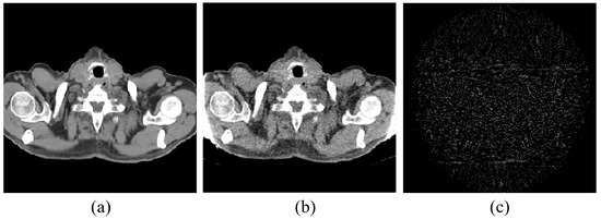
Figure 1.
Pelvic image for the experiments: (a) the target image; (b) the prior image; and (c) the difference image between the prior image and the target image.
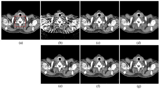
Figure 2.
48 views reconstruction results of pelvic image: (a) ground truth, (b) FBP, (c) OS-SART, (d) TV, (e) PICCS, (f) TVPI-G, and (g) NPICCS. The display window is [−150 250] HU.
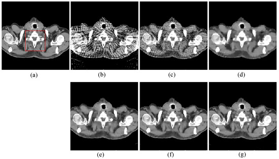
Figure 3.
64 views reconstruction results of pelvic image: (a) ground truth, (b) FBP, (c) OS-SART, (d) TV, (e) PICCS, (f) TVPI-G, and (g) NPICCS. The display window is [−150 250] HU.
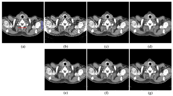
Figure 4.
80 views reconstruction results of pelvic image: (a) ground truth, (b) FBP, (c) OS-SART, (d) TV, (e) PICCS, (f) TVPI-G, and (g) NPICCS. The display window is [−150 250] HU.
To compare the recovery of reconstructed image details and edge information, we selected two regions of interest (ROIs) from the 48-view and 64-view reconstructed images and zoomed in to show. The ROIs are labelled with red box as shown in Figure 2a and Figure 3a. The corresponding zoomed-in results are shown in Figure 5. As can be seen from the figure, our algorithm can reconstruct some small image structures shown by the arrows, which are difficult to see by other algorithms. Also, we find that our algorithm performs better in edge retention.
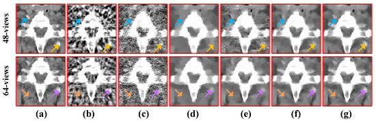
Figure 5.
The ROIs from 48-views and 64-views reconstruction results. The first row is from 48-views ROI. The second row is from 64-views ROI. (a) ground truth, (b) FBP, (c) OS-SART, (d) TV, (e) PICCS, (f) TVPI-G, and (g) NPICCS. The display window is [−150 250] HU.
To visualize the accuracy of our proposed method for local reconstruction of CT images, we plot the one-dimensional line intensity distribution of CT images reconstructed from 80 projections at two areas (shown by the blue and red lines in Figure 4a), as displayed in Figure 6. It can be visually observed that the line intensity distribution of the reconstructed images from our proposed method is closest to the original CT images at the two areas. In comparison, the proposed reconstruction algorithm has higher accuracy.
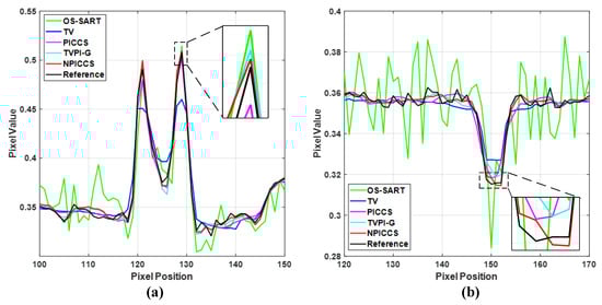
Figure 6.
Line intensity distribution of CT images reconstructed from 80-views at two areas. (a) Red line; (b) Blue line.
Next, to further show the accuracy of the global reconstruction results, Figure 7 shows the absolute difference image comparison for 48-views reconstruction. It is commonly known that the smaller the absolute difference value, the greater the accuracy of the reconstructed image. As can be seen from the Figure 7f, we can see that our result achieves the smaller absolute difference, which means our image reconstruction accuracy are better than other methods. In addition, we use RMSE, SSIM, and PSNR to compare the algorithms quantitatively. Table 1 shows the final metrics calculation result. Numerically, it can be seen that our method performs better in all three metrics, further demonstrating the superiority of the proposed algorithm.
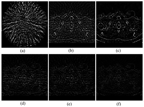
Figure 7.
Absolute difference image of different methods from 48-views. (a) FBP, (b) OS-SART, (c) TV, (d) PICCS, (e) TVPI-G, and (f) NPICCS.

Table 1.
Comparison of metrics under different views by different algorithms.
It is well known that determining the optimal parameter is a difficult problem for iterative CT reconstruction algorithm. The parameters a, γ1 and γ2 in this work are determined by extensive experiments. We use PSNR and SSIM as the basis for selecting parameters. In our experiments, optimal parameters are close at different angles, so we set parameters as the same values for different angles. Different settings of these parameters could lead to different qualities of reconstructed images. In order to study the performance of our algorithm under different parameters, we only relax one or two free parameters while fixing the other parameters. During the experiment, we firstly set a smaller initial value empirically and observe the image quality, then it is found that the image is full of strong noise and artifacts. If the parameter values increase gradually, image quality is improved and the PSNR and SSIM values rise. However, if the values increase unrestrictedly, the image quality does not improve as expected—then, the image appears to be oversmoothed and to have lost details, at the same time the PSNR and SSIM values are also significantly decreased. The parameters selection experiments are conducted and relevant quantification curves are displayed in Figure 8. From the figure, it could be observed that the parameter values have a great impact on the image quality. If the values are too high or too low, the image quality will be affected greatly. Concretely speaking, when a is 0.5, the PSNR and SSIM achieve the best value. γ1 and γ2 control the quality of the reconstructed images; it can be seen from the figure that when the values increase, the PSNR and SSIM will be higher, but if the values continue to increase, the indicators will obtain unsatisfactory results.
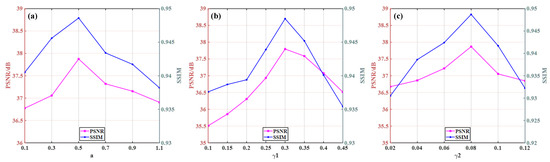
Figure 8.
Parameters selection of pelvic image: (a) parameter a; (b) parameter γ1; and (c) parameter γ2.
4.2. Image Reconstruction Experiment of Abdomen Image
The second image reconstruction experiment is conducted on an abdomen image with more image details to show the feasibility of our algorithm for SVCT reconstruction, as shown in Figure 9. We extracted 80, 64, and 48 views from a full scan and set the parameters as follows: a = 0.5, γ1 = 0.1, and γ2 = 0.06. The reconstructed results using different algorithms are shown in Figure 10, Figure 11 and Figure 12. As can be seen from the figures, our algorithm performs better than other algorithms in preserving small structures and reducing noise. Specifically, FBP reconstruction results contain severe artifacts as displayed in Figure 10b, Figure 11b and Figure 12b. OS-SART reconstruction results also have obvious noise as displayed in Figure 10c, Figure 11c and Figure 12c. TV has a better performance than FBP and OS-SART, but the result has blocky artifacts, as displayed in Figure 10d, Figure 11d and Figure 12d. The PICCS and TVPI-G algorithms have an improvement in image quality, but fine image structures are losing detail and some edge information is blurring, as displayed in Figure 10e,f, Figure 11e,f and Figure 12e,f. As can be observed from Figure 10g, Figure 11g and Figure 12g, the proposed algorithm performs better not only in preserving edge and image details, but also in reducing noise.
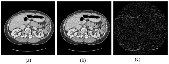
Figure 9.
Abdomen image for the experiments: (a) the target image; (b) the prior image; and (c) the difference image between the prior image and the target image.
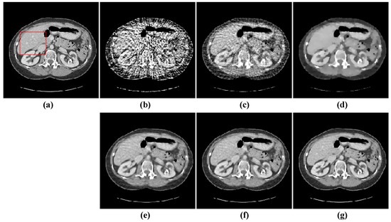
Figure 10.
48-views reconstruction results of abdomen image: (a) ground truth, (b) FBP, (c) OS-SART, (d) TV, (e) PICCS, (f) TVPI-G, and (g) NPICCS. The display window is [−150 250] HU.
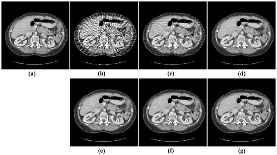
Figure 11.
64-views reconstruction results of abdomen image: (a) ground truth, (b) FBP, (c) OS-SART, (d) TV, (e) PICCS, (f) TVPI-G, and (g) NPICCS. The display window is [−150 250] HU.
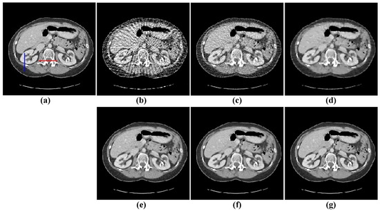
Figure 12.
80-views reconstruction results of abdomen image: (a) ground truth, (b) FBP, (c) OS-SART, (d) TV, (e) PICCS, (f) TVPI-G, and (g) NPICCS. The display window is [−150 250] HU.
Subsequently, we select two ROIs, marked by a red box as shown in Figure 10a and Figure 11a, and zoom in on them to show the results. The enlarged ROIs are shown in Figure 13. It could be observed that our algorithm can reconstruct some of the important tissues shown by the arrows, which are blurred or difficult to see in other ROIs. To show the accuracy of the different methods for local reconstruction of CT images, we plot the 1D line intensity distribution in CT images reconstructed from 80 projections in two regions (shown as blue and red lines in Figure 12a); the curves are as shown in Figure 14. Visually, it can be seen that the line intensity distribution of the image reconstructed by the proposed method is the closest to the original CT image in these two regions. In comparison, the proposed reconstruction algorithm in this paper is more accurate. At the same time, the red enlarged part of the figure indicates the edge area, from which it can be seen that the proposed algorithm has better performance in edge protection.
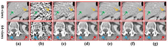
Figure 13.
The ROIs from 48-views and 64-views reconstruction results. The first row is from 48-views ROI. The second row is from 64-views ROI. (a) ground truth, (b) FBP, (c) OS-SART, (d) TV, (e) PICCS, (f) TVPI-G, and (g) NPICCS. The display window is [−150 250] HU.
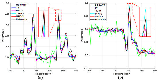
Figure 14.
Line intensity distribution of CT images reconstructed from 80 projections at two areas: (a) red line; and (b) blue line.
To show the global reconstruction accuracy, the absolute difference images are utilized to compare and are displayed in Figure 15. It could be seen that our results obtain the smallest absolute difference. Next, we utilize PSNR, RMSE, and SSIM to evaluate the algorithms from numerical indicators, as displayed in Table 2. As can be seen from the table, our algorithm performs better in all three metric values, which illustrates the advantage of our algorithm.
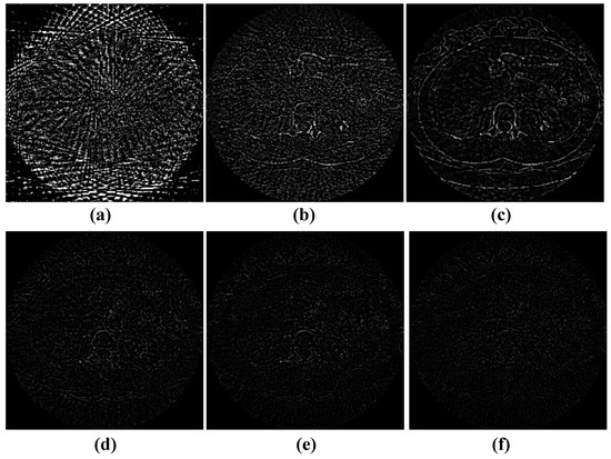
Figure 15.
Absolute difference image of different methods from 48-views. (a) FBP, (b) OS-SART, (c) TV, (d) PICCS, (e) TVPI-G, and (f) NPICCS.
Table 2.
Comparison of metric values by different algorithms.
As in the pelvic image reconstruction, we use the same method to select parameters, and the optimal parameters for reconstruction are the same at three angles; the relevant quantification curves are shown in Figure 16. The same conclusion can be drawn that the parameter values have an important impact on the image quality. When the parameters are too large or too small, the desired results are not achieved.
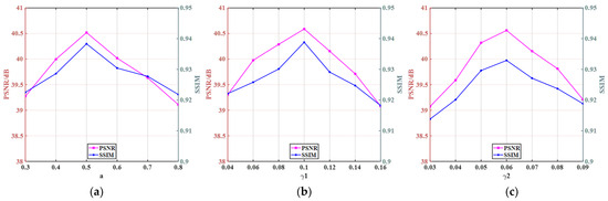
Figure 16.
Parameters selection of the abdomen image: (a) parameter a; (b) parameter γ1; and (c) parameter γ2.
5. Discussion and Conclusions
SVCT reconstruction has become a hot research topic because of its huge promise in terms of radiation dose reduction. The PICCS theory has made a great contribution to the research area. Nonetheless, the traditional PICCS-based CT reconstruction algorithms still use TV sparse framework, and the gradient L1-norm may cause blurred edges and lose image details. To resolve the limitation of the PICCS-based methods, this paper presents a novel improved PICCS algorithm for SVCT reconstruction. Firstly, the method utilizes the advantages of PICCS by introducing a prior image, which preserves more details and structures. Moreover, the algorithm incorporates the gradient L0-norm into the framework, which improves the ability of retaining edge and suppressing noise. The reconstruction results show that the proposed algorithm outperforms methods such as FBP, OS-SART, TV, PICCS, and TVPI-G.
Although the method achieves better performance, there still exist some problems. Firstly, the optimal parameters are selected by an empirical approach in this paper. Thus, how to automatically optimize the parameters needs to be investigated. Moreover, a good-quality prior image is often not available, and we get the prior image from a full-view projection with noise by direct FBP reconstruction, but noise still exists in the prior image that will affect the final image quality. In addition, it is also hard to obtain a full-view projection reconstruction image. Therefore, how to achieve a better prior image remains to be investigated. These problems will be studied in our next work. In the future, it will be fascinating to combine deep learning techniques with mathematical optimization models to improve CT image quality.
Author Contributions
Conceptualization, X.L.; methodology, X.L. and X.S.; software, X.L., F.L. and X.S.; validation, X.L., F.L. and X.S.; resources, X.L. and F.L.; writing—original draft preparation, X.L.; writing—review and editing, X.L.; funding acquisition, F.L. All authors have read and agreed to the published version of the manuscript.
Funding
This research was supported by the Natural Science Foundation for Young Scientists of Shanxi Province (202203021212455), the Shanxi Key Research and Development Program (201703D221033-3), and the Shanxi Agricultural University Young Science and Technology Innovation Program (2019021).
Informed Consent Statement
Not applicable.
Data Availability Statement
Data in this paper are available here: http://www.aapm.org/GrandChallenge/LowDoseCT/, accessed on 2016.
Conflicts of Interest
The authors declare no conflict of interest.
References
- Wang, G.; Yu, H.; De Man, B. An outlook on x-ray CT research and development. Med. Phys. 2008, 35, 1051–1064. [Google Scholar] [CrossRef] [PubMed]
- Nakano, M.; Haga, A.; Kotoku, J.; Magome, T.; Masutani, Y.; Hanaoka, S.; Kida, S.; Nakagawa, K. Cone-beam CT reconstruction for non-periodic organ motion using time-ordered chain graph model. Radiat. Oncol. 2017, 12, 145. [Google Scholar] [CrossRef]
- Brenner, D.J.; Hall, E.J. Computed tomography—An increasing source of radiation exposure. N. Engl. J. Med. 2013, 357, 2277–2284. [Google Scholar] [CrossRef] [PubMed]
- González, A.B.D.; Darby, S. Risk of cancer from diagnostic X-rays: Estimates for the UK and 14 other countries. Lancet 2004, 363, 345–351. [Google Scholar] [CrossRef] [PubMed]
- Gao, Y.; Bian, Z.; Huang, J.; Zhang, Y.; Niu, S.; Feng, Q.; Chen, W.; Liang, Z.; Ma, J. Low-dose X-ray computed tomography image reconstruction with a combined low-mAs and sparse-view protocol. Opt. Express 2014, 22, 15190–15210. [Google Scholar] [CrossRef] [PubMed]
- Kim, Y.; Kudo, H. Nonlocal Total Variation Using the First and Second Order Derivatives and Its Application to CT image Reconstruction. Sensors 2020, 20, 3494. [Google Scholar] [CrossRef] [PubMed]
- Gao, Y.; Lu, S.; Shi, Y.; Chang, S.; Zhang, H.; Hou, W.; Li, L.; Liang, Z. A Joint-Parameter Estimation and Bayesian Reconstruction Approach to Low-Dose CT. Sensors 2023, 23, 1374. [Google Scholar] [CrossRef] [PubMed]
- Kaganovsky, Y.; Li, D.; Holmgren, A.; Jeon, H.; MacCabe, K.P.; Politte, D.G.; O’Sullivan, J.A.; Carin, L.; Brady, D.J. Compressed sampling strategies for tomography. J. Opt. Soc. Am. A 2014, 31, 1369–1394. [Google Scholar] [CrossRef]
- Pan, X.; Sidky, E.Y.; Vannier, M. Why do commercial CT scanners still employ traditional, filtered back-projection for image reconstruction? Inverse Probl. 2008, 25, 1230009. [Google Scholar] [CrossRef] [PubMed]
- Gordon, R.; Bender, R.; Herman, G.T. Algebraic reconstruction techniques (ART) for three-dimensional electron microscopy and x-ray photography. J. Theor. Biol. 1970, 29, 471–476, IN1–IN2, 477–481. [Google Scholar] [CrossRef]
- Andersen, A.H.; Kak, A.C. Simultaneous Algebraic Reconstruction Technique (SART): A Superior Implementation of the ART Algorithm. Ultrason. Imaging 1984, 6, 81–94. [Google Scholar] [CrossRef] [PubMed]
- Dempster, A.P.; Laird, N.M.; Rubin, D.B. Maximum likelihood from incomplete data via the EM algorithm. J. R. Stat. Soc. Ser. B (Methodol.) 1977, 39, 1–22. [Google Scholar] [CrossRef]
- Sidky, E.Y.; Kao, C.M.; Pan, X. Accurate image reconstruction from few-views and limited-angle data in divergent-beam CT. J. X-Ray Sci. Technol. 2006, 14, 119–139. [Google Scholar] [CrossRef]
- Sidky, E.Y.; Pan, X. Image reconstruction in circular cone-beam computed tomography by constrained, total-variation minimization. Phys. Med. Biol. 2008, 53, 4777–4807. [Google Scholar] [CrossRef]
- Rudin, L.I.; Osher, S.; Fatemi, E. Nonlinear total variation based noise removal algorithms. Phys. D Nonlinear Phenom. 1992, 60, 259–268. [Google Scholar] [CrossRef]
- Tian, Z.; Jia, X.; Yuan, K.; Pan, T.; Jiang, S.B. Low-dose CT reconstruction via edge-preserving total variation regularization. Phys. Med. Biol. 2011, 56, 5949–5967. [Google Scholar] [CrossRef]
- Kim, H.; Chen, J.; Wang, A.; Chuang, C.; Held, M.; Pouliot, J. Non-local total-variation (NLTV) minimization combined with reweighted L1-norm for compressed sensing CT reconstruction. Phys. Med. Biol. 2016, 61, 6878–6891. [Google Scholar] [CrossRef]
- Liu, Y.; Ma, J.; Fan, Y.; Liang, Z. Adaptive-weighted total variation minimization for sparse data toward low-dose x-ray computed tomography image reconstruction. Phys. Med. Biol. 2012, 57, 7923–7956. [Google Scholar] [CrossRef]
- Niu, S.; Gao, Y.; Bian, Z.; Huang, J.; Chen, W.; Yu, G.; Liang, Z.; Ma, J. Sparse-view x-ray CT reconstruction via total generalized variation regularization. Phys. Med. Biol. 2014, 59, 2997. [Google Scholar] [CrossRef]
- Yu, W.; Peng, W.; Yin, H.; Wang, C.; Yu, K. Low-dose computed tomography reconstruction regularized by structural group sparsity joined with gradient prior. Signal Process. 2021, 182, 107945–107954. [Google Scholar] [CrossRef]
- Xu, Q.; Yu, H.Y.; Mou, X.Q.; Zhang, L.; Hsieh, J.; Wang, G. Low-dose X-ray CT reconstruction via dictionary learning. IEEE Trans. Med. Imaging 2012, 31, 1682–1697. [Google Scholar] [CrossRef] [PubMed]
- Dong, Y.; Hansen, P.C.; Kjer, H.M. Joint CT Reconstruction and Segmentation With Discriminative Dictionary Learning. IEEE Trans. Comput. Imaging 2018, 4, 528–536. [Google Scholar] [CrossRef]
- Gui, Y.; Zhao, X.; Bai, Y.; Zhao, R.; Li, W.; Liu, Y. Low-dose CT iterative reconstruction based on image block classification and dictionary learning. Signal Image Video Process. 2023, 17, 407–415. [Google Scholar] [CrossRef]
- Wu, J.; Dai, F.; Hu, G.; Mou, X. Low dose CT reconstruction via L1 norm dictionary learning using alternating minimization algorithm and balancing principle. J. X-Ray Sci. Technol. 2018, 26, 603–622. [Google Scholar] [CrossRef]
- Zhi, S.; Kachelrie, M.; Mou, X. Spatiotemporal structure-aware dictionary learning-based 4D CBCT reconstruction. Med. Phys. 2021, 48, 6421–6436. [Google Scholar] [CrossRef]
- Bao, P.; Sun, H.; Wang, Z.; Zhang, Y.; Xia, W.; Yang, K.; Chen, W.; Chen, M.; Xi, Y.; Niu, S.; et al. Convolutional Sparse Coding for Compressed Sensing CT Reconstruction. IEEE Trans. Med. Imaging 2019, 38, 2607–2619. [Google Scholar] [CrossRef]
- Li, X.; Li, Y.; Chen, P.; Li, F. Combining convolutional sparse coding with total variation for sparse-view CT reconstruction. Appl. Opt. 2022, 61, C116–C124. [Google Scholar] [CrossRef]
- Qi, Z.; Huang, S.; Nett, B.; Tang, J.; Yang, K.; Boone, J.; Chen, G. Dramatic Noise Reduction and Potential Radiation Dose Reduction in Breast Cone-Beam CT Imaging Using Prior Image Constrained Compressed Sensing (PICCS). Med. Phys. 2010, 37, 3443. [Google Scholar] [CrossRef]
- Szczykutowicz, T.P.; Chen, G.H. A Novel Denoising Method for Dual Energy CT Based on Prior Image Constrained Compressed Sensing (PICCS). Med. Phys. 2011, 38, 3400–3401. [Google Scholar] [CrossRef]
- Lee, H.; Yoon, J.; Lee, E.; Cho, S.; Park, K.; Choi, W.; Keum, K. Enhancement of 4D CBCT Image Quality Using An Adaptive Prior Image Constrained Compressed Sensing. Med. Phys. 2015, 42, 3639. [Google Scholar] [CrossRef]
- Rashed, E.A.; Kudo, H. Probabilistic atlas prior for CT image reconstruction. Comput. Methods Programs Biomed. 2016, 128, 119–136. [Google Scholar] [CrossRef] [PubMed]
- Lauzier, P.T.; Tang, J.; Chen, G. Time-resolved cardiac interventional cone-beam CT reconstruction from fully truncated projections using the prior image constrained compressed sensing (PICCS) algorithm. Phys. Med. Biol. 2012, 57, 2461–2476. [Google Scholar] [CrossRef]
- Chen, G.-H.; Tang, J.; Leng, S. Prior image constrained compressed sensing (PICCS). Proc. SPIE Int. Soc. Opt. Eng. 2008, 6856, 685618. [Google Scholar] [CrossRef]
- Chen, G.-H.; Tang, J.; Leng, S. Prior image constrained compressed sensing (PICCS): A method to accurately reconstruct dynamic CT images from highly undersampled projection data sets. Med. Phys. 2008, 35, 660–663. [Google Scholar] [CrossRef]
- Yu, Z.; Leng, S.; Li, Z.; McCollough, C.H. Spectral prior image constrained compressed sensing (spectral PICCS) for photon-counting computed tomography. Phys. Med. Biol. 2016, 61, 6707–6732. [Google Scholar] [CrossRef] [PubMed]
- Niu, S.; Zhang, Y.; Zhong, Y.; Liu, G.; Lu, S.; Zhang, X.; Hu, S.; Wang, T.; Yu, G.; Wang, J. Iterative reconstruction for photon-counting CT using prior image constrained total generalized variation. Comput. Biol. Med. 2018, 103, 167–182. [Google Scholar] [CrossRef] [PubMed]
- Wang, S.; Wu, W.; Feng, J.; Liu, F.; Yu, H. Low-dose spectral CT reconstruction based on image-gradient L0-norm and adaptive spectral PICCS. Phys. Med. Biol. 2020, 65, 245005. [Google Scholar] [CrossRef]
- Kong, H.; Lei, X.; Lei, L.; Zhang, Y.; Yu, H. Spectral CT Reconstruction Based on PICCS and Dictionary Learning. IEEE Access 2020, 8, 133367–133376. [Google Scholar] [CrossRef]
- Li, X.; Lu, C.; Yi, X.; Jia, J. Image smoothing via L0 gradient minimization. ACM Trans. Graph. 2011, 30, 1–12. [Google Scholar] [CrossRef]
- Biswas, S.; Hazra, R. A new binary level set model using L0 regularizer for image segmentation. Signal Process. 2020, 174, 107603. [Google Scholar] [CrossRef]
- Yuan, G.; Ghanem, B. L0TV: A Sparse Optimization Method for Impulse Noise Image Restoration. IEEE Trans. Pattern Anal. Mach. Intell. 2019, 41, 352–364. [Google Scholar] [CrossRef] [PubMed]
- Wu, W.; Zhang, Y.; Wang, Q.; Liu, F.; Chen, P.; Yu, H. Low-dose spectral CT reconstruction using image gradient ℓ0–norm and tensor dictionary. Appl. Math. Model. 2018, 63, 538–557. [Google Scholar] [CrossRef]
- Li, X.; Sun, X.; Zhang, Y.; Pan, J.; Chen, P. Tensor Dictionary Learning with an Enhanced Sparsity Constraint for Sparse-View Spectral CT Reconstruction. Photonics 2022, 9, 35. [Google Scholar] [CrossRef]
- Liu, Q.; Liang, D.; Song, Y.; Luo, J.; Zhu, Y.; Li, W. Augmented lagrangian-based sparse representation method with dictionary updating for image deblurring. SIAM J. Imaging Sci. 2013, 6, 1689–1718. [Google Scholar] [CrossRef]
- Elbakri, I.A.; Fessler, J.A. Statistical image reconstruction for polyenergetic X-ray computed tomography. IEEE Trans. Med. Imaging 2002, 21, 89–99. [Google Scholar] [CrossRef] [PubMed]
- Yu, W.; Wang, C.; Huang, M. Edge-preserving reconstruction from sparse projections of limited-angle computed tomography using ℓ0-regularized gradient prior. Rev. Sci. Instrum. 2017, 88, 043703. [Google Scholar] [CrossRef] [PubMed]
- Ren, D.; Zhang, H.; Zhang, D.; Zuo, W. Fast total-variation based image restoration based on derivative alternated direction optimization methods. Neurocomputing 2015, 170, 201–212. [Google Scholar] [CrossRef]
- Siddon, R.L. Fast calculation of the exact radiological path for a three-dimensional CT array. Med. Phys. 1985, 12, 252–255. [Google Scholar] [CrossRef]
- Shen, Z.; Gong, C.; Yu, W.; Zeng, L. Guided Image Filtering Reconstruction Based on Total Variation and Prior Image for Limited-Angle CT. IEEE Access 2020, 8, 151878–151887. [Google Scholar] [CrossRef]
- Wang, Z.; Bovik, A.C.; Sheikh, H.R.; Simoncelli, E.P. Image quality assessment: From error visibility to structural similarity. IEEE Trans. Image Process. 2004, 13, 600–612. [Google Scholar] [CrossRef]
Disclaimer/Publisher’s Note: The statements, opinions and data contained in all publications are solely those of the individual author(s) and contributor(s) and not of MDPI and/or the editor(s). MDPI and/or the editor(s) disclaim responsibility for any injury to people or property resulting from any ideas, methods, instructions or products referred to in the content. |
© 2023 by the authors. Licensee MDPI, Basel, Switzerland. This article is an open access article distributed under the terms and conditions of the Creative Commons Attribution (CC BY) license (https://creativecommons.org/licenses/by/4.0/).