Research on the Reconfiguration Method of Space-Based Exploration Satellite Constellations for Moving Target Tracking at Sea

Abstract

In addressing the challenge of tracking moving targets at sea, our focus has been directed towards the development of a reconstruction methodology founded upon satellite orbital manoeuvres. This endeavour has led us to devise a predictive model for manoeuvres within a geographic coordinate system, alongside the creation of a three-phase orbital manoeuvre model. A Non-dominant Sorting Adaptive Memetic (NSAM) algorithm is proposed in this paper, which is a two-layer multi-objective optimization algorithm that retains the advantages of evolutionary algorithms based on the population’s evolution and has an excellent local optimization ability of local search algorithms. The proposed algorithm can be used to solve multi-objective optimization problems. By comparing the target observation results before and after the satellite reconstruction simulation, it can be concluded that the orbital manoeuvring can effectively improve the observation probability and observation duration of the target at a certain speed. The orbital manoeuvre model created in this paper provides a certain methodical support for the tracking problem of moving targets at sea.

1. Introduction

Since the beginning of the 21st century, the competition in the global marine field has become increasingly fierce, and the maritime issues are complex and changeable. A question of how to speed up the construction of a maritime power and build a strong maritime force has become the development theme of all countries. With the development of modern information war, space has become the commanding height of reconnaissance and surveillance. The reasonable use of satellites to carry out maritime target tracking will enable the countries to take the lead in maritime military activities; thus, the maritime moving target tracking technology has become the focus of all the major countries. Compared with land-based, sea-based, and air-based detection means, space-based detection satellites have the advantages of wider coverage area, higher security, stronger concealment, and no restriction of national boundaries [1].

Berry [2] defined the three phases of maritime moving target tracking as “search, localization, and tracking”, and realized the tracking task of maritime moving targets through the scheduled planning of satellites in each task phase. Xu [3] obtained the optimal moving target tracking scheme by selecting and scheduling satellite observation strips and transit windows based on a target’s prior information. Automatic Identification System (AIS) assisted satellite images are used by Liu [4] to design a multi-feature track association algorithm based on Iterative Closest Point (ICP) and Global Nearest Neighbor (GNN), which provide a new method for tracking moving targets at sea. Shand [5] has realized the target tracking by combining satellite sequence images with information on a ship’s position. A multi-channel and multi-target search method, based on reinforcement learning, was proposed by Li [6] to solve the problem of satellite searching for moving targets at sea. A nine-cell adjacent observation field of view algorithm for tracking moving targets of high-orbit satellites was designed by Huang [7] to improve the utilization of the observation field of view and save a number of satellite attitude manoeuvres. The sea manoeuvring target has the characteristics of a wide range of movement and strong manoeuvrability. Due to the limitation of the orbit period of the satellite movement, the overhead imaging time cannot be controlled freely; thus, it is very difficult for space-based detection satellites to track and monitor manoeuvring targets at sea. Missing imaging opportunity may lead to the failure of the tracking task. Under this condition, if the satellite has the ability of in-orbit manoeuvring for emergency reconstruction of satellite constellation according to mission requirements, the moving target tracking task will be better completed. Furthermore, Yuanzhuo Ci [8] proposed to use a “smart satellite” to solve the problem of tracking moving targets. Yifan Xu [3] assumed that it is necessary to establish a joint scheduling technology for moving target surveillance at sea suitable for smart satellites, since the application of “smart” satellites increases the complexity of the scheduling problem. A manoeuvring target search strategy based on satellite reconstruction phase-modulated networking is proposed by Zhao [9]. Morgan [10] proposed to use the Biased Random Key Genetic Algorithm (BRKGA) to optimally solve the problem of moving target tracking at sea, based on satellite reconstruction.

From previous studies, it can be seen that it is a popular trend to better solve the moving target observation problem using satellite constellation reconfiguration. In addition, Weck [11] proposed the use of an auction algorithm for satellite constellation reconfiguration. Paek [12] used genetic algorithms to optimize satellite constellation reconfiguration, while a binary certificate linear programming formulation is used by Lee [13] to optimize the constellation reconstruction process. Application of physical planning to reconfigurable constellations for disaster observations is introduced by [14]. In general, the multi-objective optimization algorithm is one of the best methods to solve the constellation reconstruction problem at present, but the problem that it can easily fall into the local optimum cannot be ignored.

In this paper, a constellation reconfiguration method based on satellite orbit manoeuvring to cope with the task of tracking moving targets at sea is proposed. The NSAM algorithm is designed to solve the local optimal problem and realize the constellation reconstruction optimization. In Section 2, the motion prediction model of the moving target at sea will be introduced. In Section 3, the three-phase orbital manoeuvring method is proposed, and its dynamic equation is given. A new multi-objective memetic algorithm based on the NSAM is introduced in detail in Section 4. In Section 5, taking ship target tracking at sea as an example, the effectiveness of the proposed method is proved by comparing non-moving satellite tracking with moving target observation at sea by means of simulation. Finally, the main findings are summarized in Section 6.

2. Manoeuvre Prediction Model for Moving Targets at Sea

2.1. Basis for Model Selection

At present, the prediction methods for moving target motion trajectory can be divided into data-driven and behaviour-driven moving target trajectory prediction methods [15]. The data-driven moving target trajectory prediction method is used to explore the hidden target behavioural characteristics behind the data using massive historical data and predicting the target’s movement trend by fusing and matching with the current location data. There are four main categories of data-driven moving target trajectory prediction methods: probabilistic statistics, neural networks, deep learning, and hybrid models. The behaviour-driven moving target trajectory prediction method is used to predict the trajectory of a certain period of time in the future according to the relevant motion characteristics of the moving target. There are two main categories of behaviour-driven moving target trajectory prediction methods: kinetic modelling and intent recognition. Data-driven methods based on massive historical trajectory data have greater potential for application in long-time trajectory dynamics prediction. The behaviour-driven approach is more explanatory and novel, but it requires too much information on the environment and target state and has the best results only in specific scenarios. Since the environmental complexity is large and the target state uncertainty is strong in the process of observing moving targets at sea; hence, this paper adopts a data-driven moving target trajectory prediction method based on data.

The typical data-driven marine moving target motion prediction methods mainly include the dead estimation method, curve fitting method, and typical path method. The navigation position prediction method has higher requirements for the prior information of a manoeuvring target and is more accurate in judging the potential area of the target. Therefore, the navigation position prediction method is adopted in this section to establish a manoeuvring target prediction model. Next, model inference is performed in two dimensions, a two-dimensional planar coordinate system and a three-dimensional spatial coordinate system. Three-dimensional spatial model reasoning is more complicated, but the reasoning idea is basically the same as that in the two-dimensional coordinate system. The predictive model reasoning in the two-dimensional planar coordinate system is first extended to the three-dimensional spatial coordinate system after the reasoning is sufficient.

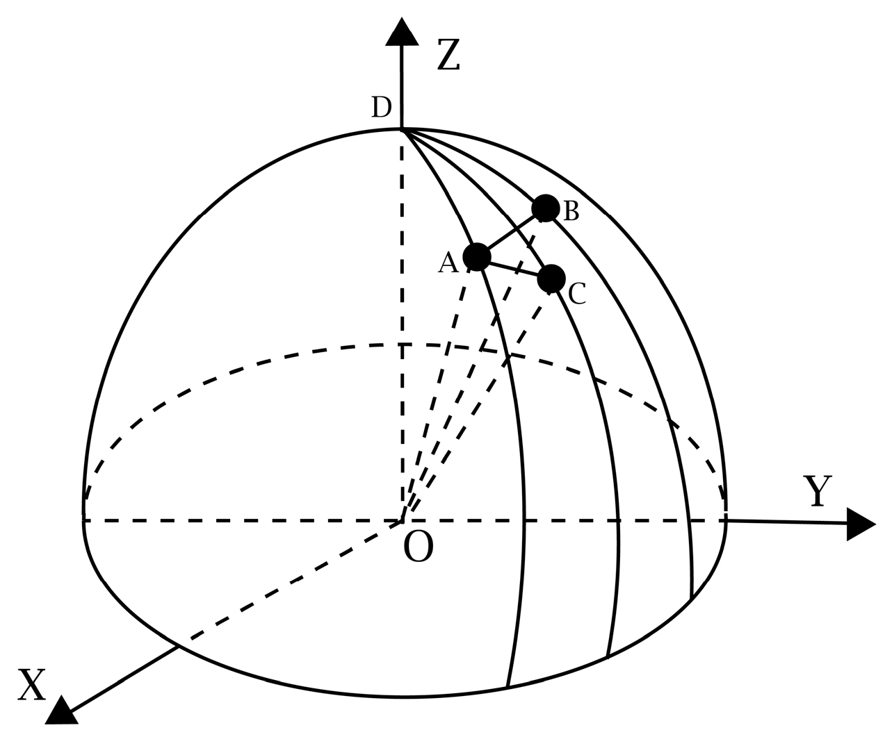
2.2. Manoeuvring Prediction Model of Moving Target in Three-Dimensional Space Coordinate System

Refer to the formula in [3]. The initial state of the moving target is known as initial position $\gamma \left({\mathrm{lon}}_{\gamma },{\mathrm{lat}}_{\gamma }\right)$, target velocity $V$, course angle $\beta$, velocity range $\pm \Delta V$, and course angle range $\pm \Delta \beta$. The possible movement area is a fan-shaped area in which movement time is $\Delta t$, with the initial position as the center of the circle; with (V − ΔV) · Δt and and $\left(V+\Delta V\right)\cdot \Delta t$ as the upper and lower boundary; and $\left(\beta -\Delta \beta ,\beta +\Delta \beta \right)$ as the azimuth range. Since the target velocity $v$ and course angle α follow the Gaussian distribution:

$$v~N\left(V,{\sigma }_V^2\right),\alpha ~N\left(\beta ,{\sigma }_V^2\right)$$

(1)

the target speed and course angle probability density can be expressed as:

$$\{\begin{array}{l}f\left(v\right)=\frac{1}{\sqrt{2\pi }{\sigma }_V}{\mathrm{e}}^{-\frac{{(v-1)}^2}{2{\sigma }_V^2}}\hfill \\ f\left(\alpha \right)=\frac{1}{\sqrt{2\pi }{\sigma }_{\beta }}{\mathrm{e}}^{-\frac{{(\alpha -\beta )}^2}{2{\sigma }_{\beta }^2}}\hfill \end{array}$$

(2)

Build the polar equation, set the movement time $\Delta t$, distance of movement $r$, and course angle $\alpha$. The joint probability density function with $r$ and $\alpha$ can be expresses as follows:

$$f\left(r,\alpha \right)=\frac{1}{\sqrt{2\pi }{\sigma }_r}{\mathrm{e}}^{-\frac{{(r-1)}^2{y}^2}{2{\sigma }_{ϵ}^2}}\cdot \frac{1}{\sqrt{2\pi }{\sigma }_{\beta }}{\mathrm{e}}^{-\frac{{(\sigma -\beta )}^2}{2\sigma {\sigma }_{\beta }}}$$

(3)

It can also be converted to rectangular coordinate equation as follows:

$$f\left(x,y\right)=\frac{1}{2\pi {\sigma }_r{\sigma }_{\beta }}\exp \left(-\frac{\Delta l^2}{2{\sigma }_r^2}-\frac{\Delta {\theta }^2}{2{\sigma }_{\beta }^2}\right)$$

(4)

The target deviates from the mean distance $\Delta l$ and deviation from the mean position angle $\Delta \theta$ can be expresses as follows:

$$\{\begin{array}{l}\Delta l=\left|\sqrt{x^2+y^2}-V\Delta t\right|\hfill \\ \Delta \theta =\left|\arctan \frac{y}{x}-\beta \right|\hfill \end{array}$$

(5)

Set the target position is (x_n, y_n) at $t_n$. After $\Delta t$, the motion distribution probability density function of moving to the $R$ region at $t_{n+1}$ is established as follows:

$$P((x_n,y_n),R,t_{n+1}-t_n)=\frac{1}{2\pi {\sigma }_r{\sigma }_{\beta }}{\displaystyle \int \underset{R}{\int }\exp (-\frac{\Delta l^2}{2{\sigma }_r^2}-\frac{\Delta {\theta }^2}{2{\sigma }_{\beta }^2})d{x}_{n+1}}d{y}_{n+1}$$

(6)

2.3. Manoeuvring Prediction Model of Moving Target in Two-Dimensional Space Coordinate System

In reality, the environment of the moving target at sea is the Earth’s surface; therefore, it is necessary to extend the prediction model to the three-dimensional coordinate system. As shown in Figure 1, set the initial position at $t_n$ as $A\left(x_n,y_n,z_n\right)$ and the position at $t_{n+1}$ as B(x_n+1, y_n+1, z_n+1). The spherical angle $\angle CAD$ is the mean course angle $\beta$; arc length $\widehat{AC}$ is the mean distance of the moving target $\widehat{AC}=V\left(t_{n+1}-t_n\right)$. The target deviates from the mean distance $\Delta l$ and deviation from the mean position angle $\Delta \theta$ are determined by geometric relations:

$$\Delta l=\left|\stackrel{⌢}{AB}\right|-\left|\stackrel{⌢}{AC}\right|=R_C\arccos \left(\frac{x_{n+1}{x}_n+y_{n+1}{y}_n+z_{n+1}{z}_n}{R_C^2}\right)-\mathrm{V}\left(t_{n+1}-t_n\right)$$

(7)

$$\Delta \mathsf{\theta }=\angle CAD-\angle \mathrm{BAD}$$

(8)

Therefore, in the three-dimensional space coordinate system, the probability that the moving target moves from position $A$ at $t_n$ to position $B$ at $t_{n+1}$ is established as follows:

$$P_r\left(A,B,t_{n+1}-t_n\right)=\frac{1}{2\pi {\sigma }_r{\sigma }_{\beta }}\exp \left(-\frac{\Delta l^2}{2{\sigma }_r^2}-\frac{\Delta {\theta }^2}{2{\sigma }_{\beta }^2}\right)$$

(9)

The probability of target distribution transferred to a certain region can be solved using integration.

3. Modelling of Three-Phase Orbital Manoeuvring Method

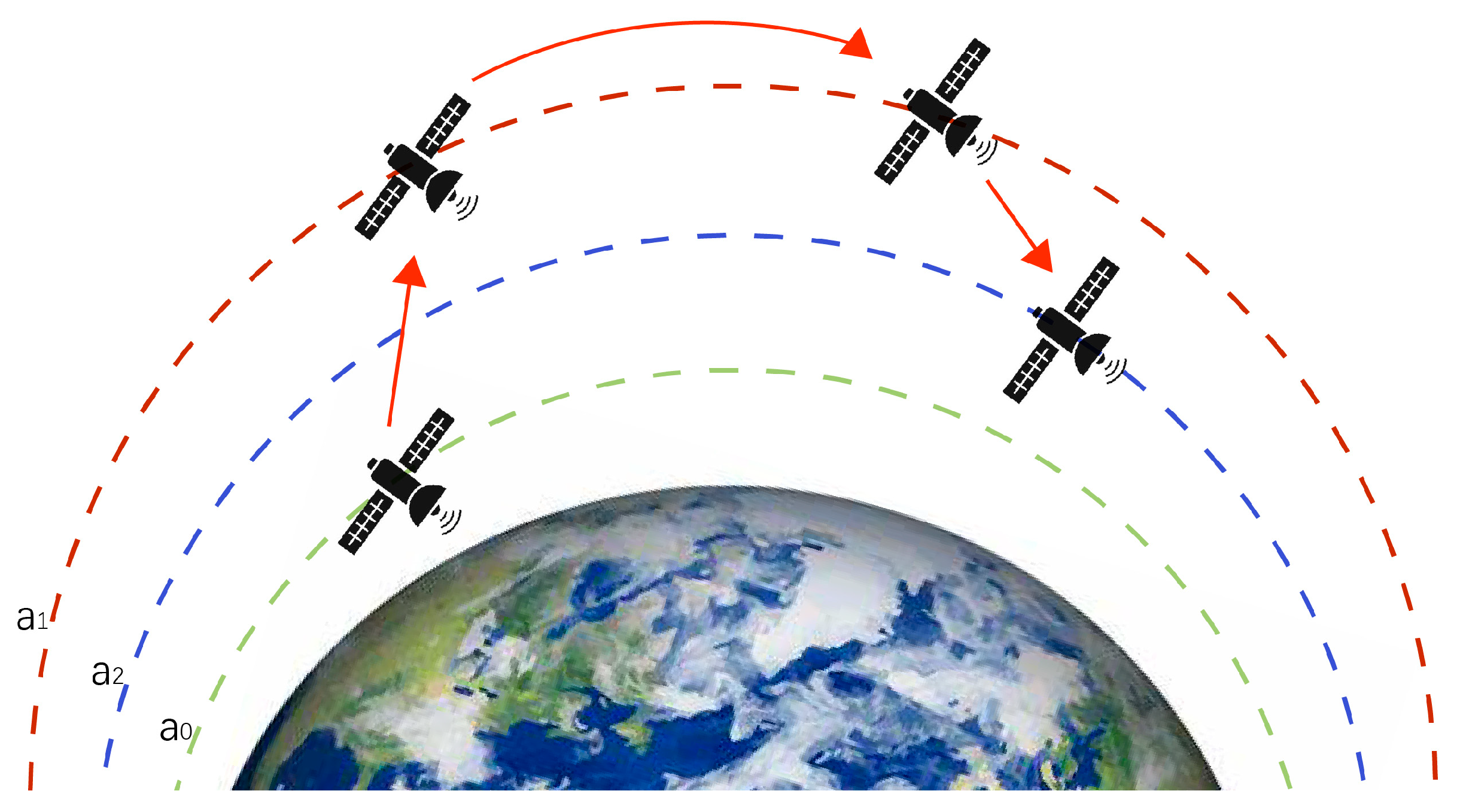
3.1. Initial Orbital Model

For the better functioning of the observation satellite, the low Earth orbit (LEO) was chosen as the initial orbit. The orbital parameters were downloaded from the UCS Satellite Database. The selection of constraints is based on the observation target area to ensure that the orbit covers the latitude region of +/− 20 degrees in the South China Sea, using the orbital parameters given in

Table 1. Spacecraft orbit parameters.

Parameter	Value	Unit
Altitude	703	km
Inclination	40	deg
Right ascension of the ascending node at epoch	0	deg
Argument of latitude at epoch	0	deg

.

During orbital motion, there are many perturbations in LEO of which the J2 term perturbation of the Earth’s oblateness is one of the most dominant long-term perturbations [16]. It directly causes long-term changes in the satellite’s Right Ascension of the Ascending Node (RAAN), Argument of Latitude (AOL), perigee radial angle, and flat perigee angle [17,18,19]. For more accurate modelling of orbital motion, the J2 effect should be considered, while the remaining latitudinal harmonics are more than 100 times smaller than the J2 perturbation [20]. Therefore, they are not considered in this paper. Other perturbations include atmospheric drag, third body effects, and solar radiation pressure. Atmospheric resistance is the most important [21].

Set the preliminary orbit as ${\dot{\mathsf{\Omega }}}_1$, argument of perigee as ${\dot{\mathsf{\omega }}}_1$, average rate of abnormal change as ${\dot{\mathrm{M}}}_1$, and average angular velocity of the satellite as $n_1$. The period of the initial orbit is established as follows:

$$T_{p_1}=\frac{2\mathsf{\pi }}{n_1+{\dot{\mathrm{M}}}_1+{\dot{\mathsf{\omega }}}_1}$$

(10)

${\dot{\mathsf{\Omega }}}_1,{\dot{\mathsf{\omega }}}_1,$ and ${\dot{\mathrm{M}}}_1$ are expressed as the following:

$${\dot{\mathsf{\omega }}}_1=\xi n_1\left(4-5{\sin }^{2}i\right)$$

(11)

$${\dot{\mathsf{\Omega }}}_1=-2\xi n_1\cos i$$

(12)

$${\dot{\mathrm{M}}}_1=-\xi n_1\left(3{\sin }^{2}i-2\right)$$

(13)

among which $\xi =\frac{3R_e^2{J}_2}{4r_1^2}$, $R_e$ represents the mean radius of the Earth, and $J_2=1.082626\times {10}^{-3}$ [22].

3.2. Three-Phase Orbital Manoeuvring Model

There is a common feature in all previous studies of constellation deployment: energy fuel consumption minimization was one of the most significant criteria [23]. Therefore, low-thrust technology is used to reduce the fuel consumption of orbital manoeuvring in this paper [24]. A three-phase orbital manoeuvre model is used in this paper. The manoeuvring strategy corresponding to the model is to use the natural orbital motion of the satellite to achieve the desired changes in the observation of the satellite’s subsatellite points. The natural disturbance size of satellite orbit is related to the satellite height; therefore, the disturbance is used to achieve the desired change of satellite orbit and change the satellite height, to achieve the change of ground orbit. Figure 2 shows the three-phase orbital manoeuvre model.

• Phase 1: the satellite maintains a constant acceleration using constant low thrust, causing the satellite orbit to increase or decrease in altitude relative to the initial orbit to a transfer orbit.
• Phase 2: satellites maintain a constant altitude in transfer orbit by counteracting the effects of atmospheric drag with thrust.
• Phase 3: the satellite is moved to the desired final altitude by using the same constant low thrust as in the first phase to give the satellite constant acceleration.

3.3. Orbital Manoeuvre Parsing

As introduced in Section 3.1, the three-phase manoeuvre is based on perturbations to achieve desired changes in the satellite orbits. Satellite perturbations will directly cause long-term changes in the RAAN and AoL. Therefore, analytical expressions are created by using RAAN and AoL as functions of the total time required for manoeuvring and the total velocity change (∆V). In order to create a complete analytic formula that can be solved quickly, it is necessary to consider the long-term orbit disturbance, which mainly includes four aspects: Earth’s non-spherical gravitational field, additional gravitational field, atmospheric drag, and disturbance caused by solar radiation [25]. In order to create a better analytical expression, this paper assumes that the satellite thrust offsets the influence of atmospheric drag in the first phase of manoeuvring, and the influence of atmospheric drag is considered in the third phase of manoeuvring. In addition, other disturbances are ignored since they are far smaller than atmospheric drag disturbances. The analytic expression obtained is established as follows:

$${\mathsf{\Omega }}_{total}={{\displaystyle \int }}_{{\overline{a}}_0}^{{\overline{a}}_1}\frac{d\mathsf{\Omega }}{da}da+{{\displaystyle \int }}_{t_1}^{t_2}\frac{d\mathsf{\Omega }}{dt}dt+{{\displaystyle \int }}_{{\overline{a}}_2}^{{\overline{a}}_3}\frac{d\mathsf{\Omega }}{da}da$$

(14)

$$u_{total}={{\displaystyle \int }}_{{\overline{a}}_0}^{{\overline{a}}_1}\frac{d\mathrm{u}}{da}da+{{\displaystyle \int }}_{t_1}^{t_2}\frac{d\mathrm{u}}{dt}dt+{{\displaystyle \int }}_{{\overline{a}}_2}^{{\overline{a}}_3}\frac{d\mathrm{u}}{da}da$$

(15)

Ω_total and $u_{total}$ are representative of the total change in RAAN and AOL:

$$\frac{d\mathsf{\Omega }}{da}=-\frac{3\overline{n}{\overline{n}}^{\prime }{R}_e^2{J}_2}{4{\overline{a}}^{2}A}\cos i$$

(16)

$$\frac{d\mathsf{\Omega }}{dt}=-\frac{3\overline{n}{R}_e^2{J}_2}{2{\overline{a}}^2}\cos \left(i\right)$$

(17)

$$\frac{du}{da}=\frac{\overline{n}{\overline{n}}^{\text{′}}}{2A}\left(1+\frac{3R_e^2{J}_2}{4{\overline{a}}^2}\left(4-5{\sin }^{2}i\right)\right)$$

(18)

$$\frac{du}{dt}=\overline{n}+\frac{3\overline{n}{R}_e^2{J}_2}{4{\overline{a}}^2}\left(4-5{\sin }^2\left(i\right)\right)$$

(19)

Equations (17) and (19) are the expressions for RAAN and AoL over time for the second stage. Equations (16) and (18) are the expressions of RAAN and AoL as a function of the satellite half-length axis for the first and third phases, respectively, where $J_2$ is the second zonal harmonic coefficient of the gravitational coefficient of the Earth, $R_e$ is the mean radius of the Earth, and $\overline{a}$ is the mean semi-major axis.

The first stage manoeuvre time is established as follows:

$$t_1=\frac{\sqrt{\mu }\left(a_0^{5/2}\left\{20a_1^2+3J_2{R}_e^2\left[2-3{\sin }^{2}i\right]\right\}+3a_1^{5/2}{J}_2{R}_e^2\left[3{\sin }^{2}i-2\right]-20a_1^{5/2}{a}_0^2\right)}{20a_0^{5/2}{a}_1^{5/2}A}$$

(20)

The speed change of the first stage manoeuvre is established as follows:

$$\Delta V_1=\left|\sqrt{\frac{\mu }{a_1}}-\sqrt{\frac{\mu }{a_0}}\right|$$

(21)

$\mu$ is the standard gravity parameter of the Earth. The maneuvering time and velocity change of the third stage are obtained by replacing $a_0$ and $a_1$ with $a_2$ and $a_3$ in the formula of manoeuvring time and velocity change of the first stage.

4. Non-Dominant Sorting Adaptive Memetic Algorithm (NSAM)

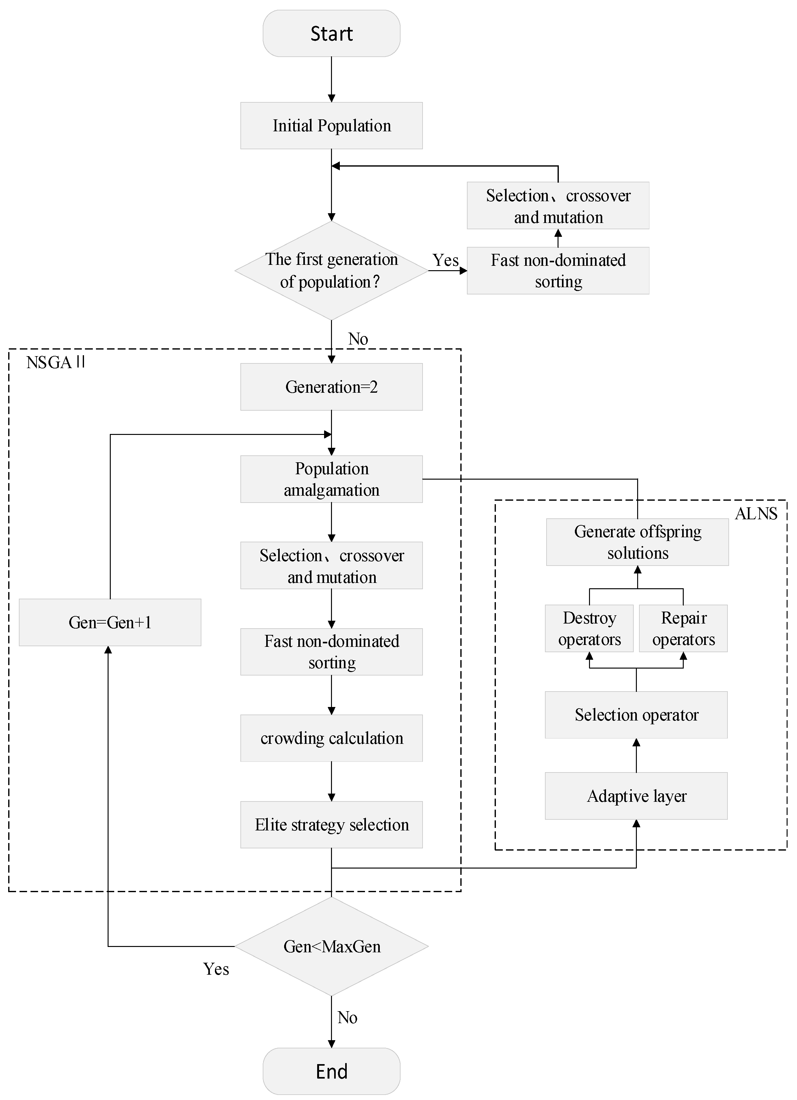
4.1. Basic Structure of the NSAM

Moscato [26] defined the Memetic Algorithm (MA) in 1989, which was initially improved on the basis of Genetic Algorithm (GA). He combined the GA with local search to solve the Travelling Salesman Problem (TSP). In recent years, with the successful and high-performance application of the two-layer search architecture of memetic algorithm on solving complex real-world problems, the concept of memetic algorithm has attracted widespread attention from the academic community [27]. Memetic algorithms are no longer a specific algorithm, but generally refer to a class of population-based heuristics. Algorithms of this type combine the evolution algorithm with the local search algorithm, so that it cannot only retain the advantages of the evolutionary algorithm based on population evolution during operation, but also has the excellent local optimization ability of the local search algorithm.

The NSAM algorithm is a two-layer modal approach comprised the Non-dominated Sorting Genetic Algorithm II (NSGA-II) and Adaptive Large Neighborhood Search (ALNS). The two-layer optimization approach not only allows the population to quickly reach the Pareto frontier using an evolutionary mechanism, but also quickly reproduces progeny solutions by improving the quality of the searched solutions using the ALNS. Thus, the generation of local optimal solutions is avoided. The NSGA [28] is a genetic algorithm based on Pareto optimal concept proposed by Srinivas et al. in 1995. Deb [29] proposed the NSGA-II algorithm on the basis of this algorithm. The algorithm greatly reduces the computation time by using fast non-dominated sorting (the elite strategy) to ensure the excellent individuals can have a higher probability of being retained; the crowding degree method replaces the fitness sharing strategy to ensure individual diversity in the population. This makes the NSGA-II algorithm more suitable for solving multi-objective optimization problems. The ALNS is a heuristic local search method proposed by Pisinger [30] in 2007. On the basis of the neighbourhood search, this method adds the measurement of operator effect. By means of roulette, the better operator of destroy and repair will be automatically selected to optimize the solution.

This two-layer architecture plays a significant role in solving highly complex and large-scale constellation reconstruction problems. The flow chart of the NSAM is shown in Figure 3. The algorithm’s code framework is shown in Algorithm 1.

Algorithm 1 NSAM algorithm
Input: target trajectory, satellite parameters, initial population size (IPS), offspring population size (OPS), and maximum iterations (MaxIter) Output: elitist solutions (ES)
1	Repeat: generate initial solution
2	According to the input elements to generate initial solutions
3	End: until parent population size = IPS + OPS
4	The solutions were optimized by selection, crossover, and mutation in $NSGA-II$
5	Select and update elite solutions with elite strategies in $NSGA-II$
6	ALNS: improve the solutions
7	Select destroy operators and repair operators according to the adaptive layer
8	Based on the current elitist solutions, use operators to update populations
9	Combine the offspring solutions and the current elitist solutions
10	Update the elite solutions and update the scores and weights of operators in the adaptive layer
11	End until iteration achieves MaxIter
12	Output

4.2. Design of Destroy Operator and Repair Operator

Destroy operators and repair operators are used to optimize the generated elite population. The destroy operator changes the population composition by deleting some target solutions, while the repair operator takes some solutions from the non-elite solutions to repair the parent solutions to generate a new population. In this paper, we designed six kinds of destroy operators and five kinds of repair operators.

4.2.1. Destroy Operators

All destroyed operators are uniformly stored in set $B$, and three different types of destroy operators are defined as follows:

R-destroy: randomly selects solutions for the existing population and deletes them.

Max-destroy: calculates the single solution by summing elements, sorts and deletes the solution with the maximum value.

Rank-destroy: deletes all the solutions whose rank value is not 0.

$\Delta V$-destroy: traverses $\Delta V$ in the solutions, sorts and deletes the solution with the maximum $\Delta V$.

Distance-destroy: traverses the distances to the target in the solutions, sorts and deletes the solution with the maximum mean distance to targets accessed.

Access-destroy: traverses the targets access time in the solutions, sorts and deletes the solution with the minimum targets access time.

4.2.2. Repair Operators

Save all non-elite solutions in set $F$. Solutions are selected from the set $F$ and inserted into the destroyed population to generate a new population, and five different types of repair operators are defined as follows:

R-repair: randomly selects several solutions from the set $F$ and inserts them into the destroyed population.

Min-repair: calculates the single solution by summing elements, sorts and inserts the solution with the minimum value.

$\Delta V$-repair: traverses $\Delta V$ in the solutions, sorts and inserts the solution with the minimum $\Delta V$.

Distance-repair: traverses the distances to the target in the solutions, sorts and inserts the solution with the minimum mean distance to targets accessed.

Access-repair: traverses the targets access time in the solutions, sorts and inserts the solution with the maximum targets access time.

4.3. Adaptive Strategy Design and Termination Criterion Design

Six kinds of destroy operators and five kinds of repair operators were designed in Section 4.2. Each operator has a score and weight, and the score and weight are updated according to the performance of the operator; thus, affecting the probability of the operator being selected. The update methods of the operator scores and weight are described as the following:

Set ${\pi }_i^d$ and ${\pi }_i^r$ as the scores of the $i^{th}$ destroy operator and repair operator; ${\omega }_i^d$ and ${\omega }_i^r$ as the weight of the $i^{th}$ destroy operator and repair operator. The score of all heuristics is set to zero at the start of each segment. We set the weights of the destroy operator ${\pi }_i^d=\frac{1}{6}$; the weights of the repair operator are the same as ${\omega }_i^r=\frac{1}{5}$. The score is used to judge the validity of the operator, the weight is used to determine the probability of the operator being selected, and the weight is updated according to the score of the operator. As for destroy operators and repair operators, each $\phi$ times iteration as a stage, and the scores of all selected operators are updated according to the returns of the new solutions at the end of each iteration. At the end of each phase, the weights of all operators are updated according to the scores accumulated by the operators in this stage, and the operator scores are initialized. The update equation for operator weights is shown:

$${\omega }_i=\left(1-\rho \right){\omega }_i+\rho \frac{{\pi }_i}{{{\displaystyle \sum }}_{i=1}^H{\pi }_i}$$

(22)

where $\rho \in \left[0,1\right]$ is the operator weight update coefficient and means the degree to which the operator is affected by historical data. The operator performance is graded in the iteration process: the higher the score the better the operator’s performance. The four kinds of changing score scenarios are set as follows:

If the new solution is better than all the other solutions: ${\sigma }_1$.

If the new solution is better than one of the current dominant solutions: ${\sigma }_2$.

If the new solution is dominated by the current solution but accepted under certain criteria: ${\sigma }_3$.

If the new solution is inferior and does not satisfy the acceptance criteria: ${\sigma }_4$.

If only the optimal solution is accepted in the search process, the risk of falling into the local optimal will be generated. Therefore, the simulated annealing method is used to accept the inferior solution with a certain probability. After getting the new weight, the operator is selected by way of roulette so that the probability of the operator being selected is proportional to the weight, and the probability of each operator being selected is shown as follows:

$$p_i=\frac{{\omega }_i}{{{\displaystyle \sum }}_{j=1}^H{\omega }_j}$$

(23)

We defined the maximum number of iterations $Maxlter$ at the beginning of the evolution which is the unique termination criterion of the algorithm.

5. Simulation Experiments

5.1. Parameter Setting

The simulation experiment background design: 27 October 2022$00:00:00$, The ship was found at the position (11.7° N, 132.0° E), and the trajectory of the ship was shown in

Table 2. Ship’s location at 0.5 day intervals.

Date	Time	Latitude	Longitude
27 October 2022	00.00	11.7	132.0
27 October 2022	12.00	11.3	131.1
28 October 2022	00.00	11.4	129.9
28 October 2022	12.00	12.1	127.2
29 October 2022	00.00	13.8	124.1
29 October 2022	12.00	13.7	121.7
30 October 2022	00.00	15.4	119.9
30 October 2022	12.00	16.1	118.3
31 October 2022	00.00	15.8	117.2
31 October 2022	12.00	16.8	117.0
1 November 2022	00.00	18.4	116.2
1 November 2022	12.00	19.1	115.9
2 November 2022	00.00	20.4	116.0
2 November 2022	12.00	21.0	115.1
3 November 2022	00.00	21.8	114.2

below:

The 3U CubeSat satellite equipped with an electrospray propulsion system [31] is selected and the satellite’s parameters are shown in

Table 3. Satellite’s physical and orbit parameters.

Parameter	Value	Unit
Mass	4	kg
Thrust	0.35	mN
The field of view of the satellite diameter	200	km

.

The parameters of the simulated Earth experiment are shown in

Table 4. The Earth’s simulation parameters.

Parameter	Value	Unit
Mean Earth radius	$6371$	km
Earth rotation rate	$7.29212\times {10}^{-5}$	rad/s
Coefficient of the Earth’s gravitational zonal harmonic of the second degree	0.00108270	-
Earth’s standard gravitational parameter	$3.986\times {10}^{14}$	${\mathrm{m}}^3/{\mathrm{s}}^2$
Flattening factor of Earth	$0.00335281$	-

.

The parameter settings of the algorithm are shown in

Table 5. The NSAM’s algorithm parameters.

Parameter	Meaning	Value
IPS	Initial population size	1150
OPS	Offspring population size	800
MaxIter	Maximum iterations	300
${\sigma }_1$	The score of the new solution is better than all the other solutions	3
${\sigma }_2$	The score of the new solution is better than one of the current dominant solutions	2
${\sigma }_3$	The score of the new solution is dominated by the current solution, but accepted under certain criteria	1
${\sigma }_4$	The score of the new solution is inferior and does not satisfy the acceptance criteria	0.5

.

5.2. Reconfiguration Analysis

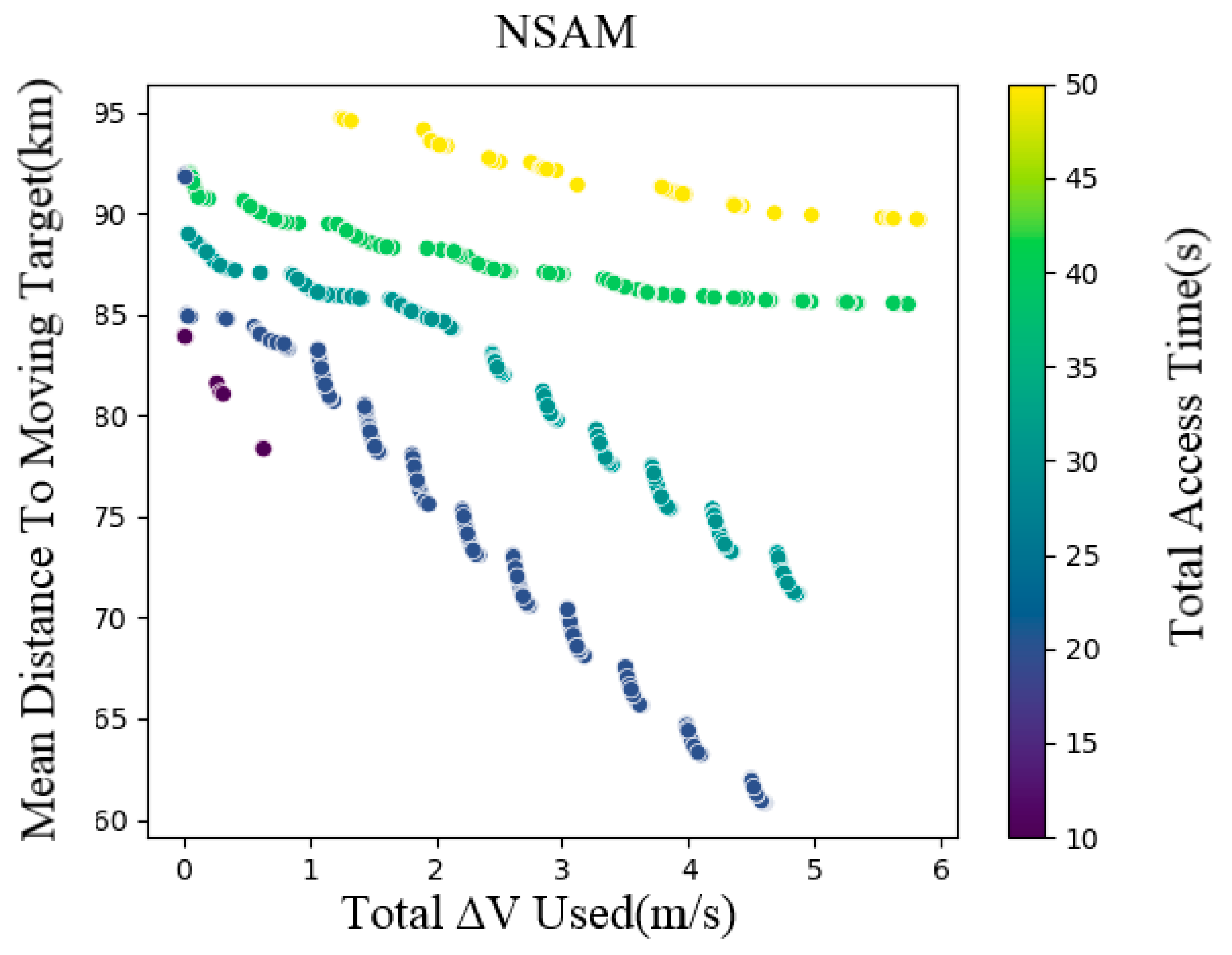
5.2.1. Analysis of the Results

A multi-objective optimization using a single satellite for a moving target at sea was performed and the set of non-dominated solutions obtained is shown in Figure 4. The dominated solutions obtained through the optimization are shown in Figure 4.

Many observation schemes are obtained through optimization. It can be concluded that, we can increase the observation time at the same average observation distance by increasing the delta-v. Similarly, for the same access time, the target was observed at a much closer distance by increasing the delta-v. The balance relationship between manoeuvrability, mean distance to the moving target, and total observation time is obtained.

The observation of moving targets at sea by non-moving satellites and moving satellites is shown in

Table 6. Comparison between non-manoeuvring and manoeuvring.

(a)
Target Number	Non-Manoeuvring
	Delta-V (m/s)	Mean Distance (km)	Total Access Time (s)	Target in View
1	-	85	30	Yes
2	-	-	-	No
3	-	86	10	Yes
4	-	59	40	Yes
5	-	76	50	Yes
Summary	0 m/s	76.5	130	-
(b)
Target Number	Manoeuvring
	Delta-V (m/s)	Mean Distance (km)	Total Access Time (s)	Target in View
1	2.06	90	50	Yes
2	0.24	91	30	Yes
3	4.968	84	30	Yes
4	4.172	59	60	Yes
5	0.466	71	60	Yes
Summary	11.91 m/s	79	230	-

. Table 6 gives a detailed description of the access situation of the target. It can be seen that in the case of no manoeuvring of a single satellite, as shown in the Table 6a, the second target point cannot be observed, and the total observation time of the target is relatively short. Compared with a non-dominated solution after manoeuvring, all the target points can be observed through manoeuvring, and the observation time is larger when the mean distance difference is small.

5.2.2. Experimental Platform Results Diagram

The results of this paper are verified on the IEAT-C platform. The experimental platform architecture diagram is shown in the Figure 5.

Its core components are as follows:

STK: provide satellite and the simulation environment of the Earth, the satellite, and ground target data and calculated data.

Ray: provide distributed computing capabilities, perform parallel or asynchronous tasks, and interact with the underlying STK to obtain simulation data.

K8s: underlying computing resource management and application hosting capabilities, STK components and Ray components are hosted on top of it.

Web: divided into frontend and backend, providing simulation environment, input and output interaction of calculation and visualization ability.

Based on the historical trajectory of the moving target, the satellite’s manoeuvring method is designed to achieve the original design intention of tracking the moving target. Inputting the manoeuvre parameters of the satellite and the geodetic coordinates of the target, the NSAM algorithm is used to calculate the maximized access time, minimized manoeuvre, and shortest access distance of the satellite to the target. According to the obtained dominant solution, the orbit parameters of the three-phases are obtained on the simulation platform, as shown in

Table 7. Three-phase orbit parameters.

Track Name	Altitude (km)	Inclination (deg)	Right Ascension of the Ascending Node at Epoch (deg)	Argument of Latitude at Epoch (deg)
Initial orbit	703	40	0	0
Transfer orbit	720	40	0	0
Final orbit	715	40	0	0

, while the effect diagram is shown in Figure 6:

6. Conclusions

In this paper, a reconfigurable constellation is designed to accomplish the task of tracking moving targets at sea. Therefore, the moving target prediction model is used to predict the trajectory of a moving target at sea. Then, with the consideration of orbital disturbance and the minimization of fuel consumption, a three-phase orbital manoeuvring method is designed. The NSAM algorithm is proposed to intelligently generate feasible solutions. The optimization algorithm plays an important role in constellation reconstruction selects the best possible trajectory option and plans the best manoeuvres. In other words, the trajectory parameters are optimized by the algorithm to obtain the global optimal mean distance, total access time, and $\Delta V$. Finally, the tracking situation of targets with or without orbital manoeuvring is compared, and the experiment is verified on the self-designed IEAT-C experimental platform. The results of this study show that the satellite manoeuvring reconstruction with low thrust can realize the tracking of sea targets and collect target data with better quality and quantity.

This paper mainly focuses on the methodology of constellation reconstruction. The research on the NSAM algorithm is still limited to the design and application of the algorithm’s structure. The comparison of algorithm’s performance has not been studied in depth. Furthermore, the advantages and disadvantages of the NSAM algorithm in the field of multi-objective optimization algorithms should be deeply studied. In addition, the number of satellites and the number of orbits should be increased to prove the universality, scalability, and adaptability of the method.

References

1. Zhu, D.; Zhang, Z.; Zhao, C. A satellite configuration design to achieve optical stealth. Space Control Technol. Appl. 2017, 43, 61–66. [Google Scholar]
2. Berry, P.E.; Fogg, D.A.B.; Pontecorvo, C. Optimal Search, Location and Tracking of Surface Maritime Targets by a Constellation of Surveillance Satellites; DSTO Information Sciences Laboratory: Canberra, Australia, 2003. [Google Scholar]
3. Yifan, X. Joint Scheduling for Space-Based Maritime Moving Targets Surveillance; National University of Defense Technology: Changsha, China, 2011; pp. 40–63, 74–125, 142–145. [Google Scholar]
4. Liu, Y.; Yao, L.; Xiong, W. GF-4 satellite and automatic identification system data fusion for ship tracking. IEEE Geosci. Remote Sens. Lett. 2018, 16, 281–285. [Google Scholar] [CrossRef]
5. Larson, K.M.; Lyndsay, S.; Andrea, S.; Skyler, G.; Erika, L.R.; Don, L. An efficient approach for tracking the aerosol-cloud interactions formed by ship emissions using GOES-R satellite imagery and AIS ship tracking information. arXiv 2021, arXiv:2108.05882. [Google Scholar]
6. Li, J.; Yao, F.; Xu, Y. Using Multiple Satellites to Search for Maritime Moving Targets Based on Reinforcement Learning. J. Donghua Univ. Engl. 2016, 33, 749–754. [Google Scholar]
7. Lixia, H.; Xin, P.; Shuhao, L.; Hua, Z. Design and simulation of moving target tracking strategy for high-orbit optical imaging satellite. Spacecr. Eng. 2018, 27, 10–16. [Google Scholar]
8. Ci, Y. Multi-Satellite Mission Planning for Moving Target Search; National University of Defense Technology: Changsha, China, 2008; pp. 88–115. [Google Scholar]
9. Chengliang, Z.; Zhanyue, Z.; Zhiliang, L.; Yao, L. Satellite Reconstruction Network Optimization and Simulation for Marine Maneuvering Target Tracking and Surveillance. Aerosp. Control Appl. 2018, 44, 1–7. [Google Scholar]
10. Morgan, S.J.; McGrath, C.; De, W.O.L. Mobile target tracking using a reconfigurable low earth orbit constellation. ASCEND 2020, 2020, 42–47. [Google Scholar]
11. Paek, S.W.; Kim, S.; De, W.O. Optimization of reconfigurable satellite constellations using simulated annealing and genetic algorithm. Sensors 2019, 19, 765. [Google Scholar] [CrossRef] [PubMed]
12. Mirjalili, S. Genetic algorithm. In Evolutionary Algorithms and Neural Networks: Theory and Applications; Springer: Berlin/Heidelberg, Germany, 2019; pp. 43–55. [Google Scholar]
13. Lee, H.W.; Ho, K. Binary integer linear programming formulation for optimal satellite constellation reconfiguration. In Proceedings of the AAS/AIAA Astrodynamics Specialist Conference, South Lake Tahoe, CA, USA, 9–13 August 2020; Volume 8. [Google Scholar]
14. He, X.; Li, H.; Yang, L.; Zhao, J. Reconfigurable satellite constellation design for disaster monitoring using physical programming. Int. J. Aerosp. Eng. 2020, 2020, 8813685. [Google Scholar] [CrossRef]
15. Liu, W.; Hu, K.; Li, Y. A review of prediction methods for moving target trajectories. Chin. J. Intell. Sci. Technol. 2021, 3, 149–160. [Google Scholar]
16. Huang, S.; Colombo, C.; Alessi, E.M. Low-thrust de-orbiting from Low Earth Orbit through natural perturbations. Acta Astron. 2022, 195, 145–162. [Google Scholar] [CrossRef]
17. Di, P.G.; Sanjurjo, R.M.; Pérez, G.D. Optimal Low-Thrust Orbital Plane Spacing Maneuver for Constellation Deployment and Reconfiguration including J2. In Proceedings of the AIAA SciTech 2022 Forum, San Diego, CA, USA, 3–7 January 2022; p. 1478. [Google Scholar]
18. Kozai, Y. The motion of a close earth satellite. Astron. J. 1959, 64, 367. [Google Scholar] [CrossRef]
19. Brouwer, D. Solution of the problem of artificial satellite theory without drag. Astron. J. 1959, 64, 378. [Google Scholar] [CrossRef]
20. Curtis, H.D. Orbital Mechanics for Engineering Students[M]; Butterworth-Heinemann: Oxford, UK, 2013. [Google Scholar]
21. Casanovas, G.F. The Reality of Space Exploration: A Complete Integral Approach of Space Mission Design; Universitat Politècnica de Catalunya: Barcelona, Spain, 2023. [Google Scholar]
22. Zhao, Z.; Zhang, J.; Li, H.; Zhou, J. LEO cooperative multi-spacecraft refueling mission optimization considering J2 perturbation and target’s surplus propellant constraint. Adv. Space Res. 2017, 59, 252–262. [Google Scholar] [CrossRef]
23. Bakhtiari, M.; Abbasali, E.; Daneshjoo, K. Minimum Cost Perturbed Multi-impulsive Maneuver Methodology to Accomplish an Optimal Deployment Scheduling for a Satellite Constellation. J. Astronaut. Sci. 2023, 70, 18. [Google Scholar] [CrossRef]
24. Changxuan, W.; Chen, Z.; Yu, C.; Dong, Q. Low-thrust transfer between circular orbits using natural precession and yaw switch steering. J. Guid. Control Dyn. 2021, 44, 1371–1378. [Google Scholar]
25. Vallado, D.A. Fundamentals of Astrodynamics and Applications; Springer Science & Business Media: Berlin/Heidelberg, Germany, 2001. [Google Scholar]
26. Macdonald, M.; Viorel, B. The International Handbook of Space Technology; Springer: Berlin/Heidelberg, Germany, 2014; Volume 3, pp. 154–196. [Google Scholar]
27. Neri, F.; Cotta, C. Memetic algorithms and memetic computing optimization: A literature review. Swarm Evol. Comput. 2012, 2, 1–14. [Google Scholar] [CrossRef]
28. Srinivas, N.; Deb, K. Muiltiobjective optimization using nondominated sorting in genetic algorithms. Evol. Comput. 1994, 2, 221–248. [Google Scholar] [CrossRef]
29. Deb, K.; Pratap, A.; Agarwal, S.; Meyarivan, T. A fast and elitist multiobjective genetic algorithm: NSGA-II. IEEE Trans. Evol. Comput. 2002, 6, 182–197. [Google Scholar] [CrossRef]
30. Pisinger, D.; Ropke, S. A general heuristic for vehicle routing problems. Comput. Oper. Res. 2007, 34, 2403–2435. [Google Scholar] [CrossRef]
31. McGrath, C.N.; Clark, R.A.; Werkmeister, A.; Macdonald, M. Small satellite operations planning for agile disaster response using graph theoretical techniques. In Proceedings of the 70th International Astronautical Congress, Washington, DC, USA, 21–25 October 2019; pp. 21–25. [Google Scholar]
Figure 1. Target motion diagram in three-dimensional coordinate system.
Applsci 13 10103 g001
Figure 2. Schematic diagram of the three-phase orbital manoeuvre. a0: initial orbit. a1: transfer orbit. a2: final orbit.
Applsci 13 10103 g002
Figure 3. Flow chart of NSAM algorithm.
Applsci 13 10103 g003
Figure 4. Non-dominated set of solution for single satellite.
Applsci 13 10103 g004
Figure 5. IEAT-C architecture diagram.
Applsci 13 10103 g005
Figure 6. Results Simulation. (a) Initial state. (b) Final state.
Applsci 13 10103 g006