A Two-Step Matheuristics for Order-Picking Process Problems with One-Directional Material Flow and Buffers

Abstract

The necessity for undertaking this research is driven by the prevailing challenges encountered in logistic centers. This study addresses a logistic order-picking issue involving unidirectional conveyors and buffers, which are assigned to racks and pickers with the objective of minimizing the makespan. Subsequently, two variations of a two-step matheuristic approach are proposed as solution methodologies. These matheuristics entail decomposing the primary order-picking problem into two subproblems. In the initial step, the problem of minimizing the free time for pickers/buffers is solved, followed by an investigation into minimizing order picking makespan. An experimentation phase is carried out across three versions of a distribution center layout, wherein one or more pickers are allocated to one or more buffers, spanning 120 test instances. The research findings indicate that employing a mathematical programming-based technique holds promise for yielding solutions within reasonable computational timeframes, particularly when distributing products to consumers with limited product variety within the order. Furthermore, the proposed technique offers the advantages of expediency and simplicity, rendering it suitable for adoption in the process of designing and selecting order-picking systems.

1. Introduction

Throughout the years, considerable attention has been directed toward the management of warehouse operations [1]. The process of locating items within a warehouse or fulfillment center and preparing them for dispatch to customers is commonly referred to as “warehouse picking”.

One of the main research priorities is order picking, which is generally defined as the recovery of goods from storage sites to fulfill customer orders [2]. This is due to two factors: first, the substantial amount of manual work that choosing orders entails [3], and second, the fact that order picking is a very time-intensive task that has a direct influence on customer service [1,4].

Today’s supply networks are under a lot of demand. There are too many elements upsetting the delicate balance in supply systems, including a lack of raw materials, bad weather, natural catastrophes, and the pandemic. This causes supply chains to break down, which can delay or even cause deliveries to be canceled. This has a significant impact on production and logistics.

Technology advancement has accelerated innovation in the supply chain to previously unheard-of levels, e.g., blockchain technology, cloud computing, the Internet of Things (IoT), and big data [5,6].

In the warehouse, sustainability has taken on more importance. When a warehouse can run in a way that is beneficial to both society and the environment, it is sustainable. It has systems in place to reduce waste, emissions, energy use, and environmental effects as a whole.

Overall, it can be said that the problem of warehouse logistics is difficult, and it is useful to utilize computer simulations, optimization, and mathematical modeling techniques for its efficient solution [7,8]. Mathematical modeling was utilized by Georgijevicet al. (2013) [7] to examine the ideal number, size, and placement of public logistics warehouses.

Most of the research investigates the order-picking problem in terms of picker-to-parts, in which the picker walks around the logistic center and picks products for the order. However, many logistic centers are functioning with zone picking rules in which the picker collects the products for selected orders only from his zone. Therefore, in this research, we investigate the process by which the container is moved via the conveyor to the consequent picking zones in which the pickers can collect the orders.

We present a practical logistic order-picking model with a one-directional conveyor and buffers to which the racks and pickers are assigned. In the investigated distribution center, three versions of the layout are modeled: (1) each picker is allocated to a single buffer; (2) one picker is allocated to more than one buffer; and (3) more than one picker is allocated to one buffer. The criteria is to minimize the total time needed to complete all orders. Therefore, by using a proposed mathematical model, it is possible to instruct the pickers in what sequence to pick products for the containers during the order-completing phase, which results in a reduction of time on later steps such as packing and shipping.

The goal of this study is to find new optimization tactics and develop two versions of the two-step matheuristic for the required order-picking problem. The proposed approach includes the decomposition of the main order picking problem into two consequent subproblems at the first step, of which the pickers/buffers free time minimization problem is solved, and at the following stage, order picking makespan minimization is solved. The acquired knowledge demonstrates the application possibilities of the proposed matheuristics in terms of increased scalability, lower operational expenses, and improved employee productivity.

The remainder of the paper is organized as follows: The next section, Section 2, presents a brief literature review. After that, a description of the investigated order-picking problem and its mathematical model are given in Section 3. Section 4 presents the new matheuristics. Section 5 reports the computational results. In Section 6, some concluding remarks and future work directions are presented.

2. Related Literature

2.1. The Importance of Sustainability in Logistics

A collection of practices known as sustainable logistics aims to lessen the negative effects of environmental degradation brought on by the operations of the logistics sector. The primary goal is to alter certain supply chain behaviors in order to strike a balance between environmental preservation and business growth.

Sustainability in business and manufacturing entails a focus on meeting the needs of an organization’s direct and indirect stakeholders, which may include a person, a corporation, a community, a city, or a government, while taking into account the interests of future stakeholders [9]. Since this is an issue that affects us all, it is crucial that businesses or organizations adopt sustainable practices.

Today’s enterprises have far easier access to cost-effective, sustainable solutions than they did in the past. However, commercial and business parameters are more prioritized in industrial paradigms than environmental considerations [10].

The industrial sector is becoming more conscious of the detrimental effects of its operations, and many businesses have already implemented efforts to reduce their environmental impact. Platform service supply chains have taken center stage in economic and social growth as platforms become more common in business operations [5]. Customers want to lower their running expenses; therefore, they search for buildings that have a strong possibility of being operationally efficient. Customers may also seek sustainable structures that are comfortable and functional.

The crucial results of supply chain innovation are online platform services [6]. A growing number of businesses from all sectors are joining online platforms or creating their own platforms to provide clients with more value-added services and boost revenues. All different types of markets, including retail, tourism, lodging, transportation, and so on, have been invaded by platform modes [11].

Investors and clients prefer buildings with sustainable elements. Companies, including those in the logistics, storage, or handling industries, have made protecting the environment and continuously seeking ways to lessen pollution and its effects one of their top concerns.

Logistics services that incorporate green components have the largest influence on how supply chains are shaped toward sustainability. Business strategies need to encourage ecologically conscious reasoning through ongoing integration of green and performance monitoring of resulting environmental and business sustainability [12].

Rapid industrialization has accelerated the atmospheric concentration of greenhouse gases, resulting in severe global climate change and ecological destruction. Chiang et al. (2023) [13] concentrated on warehouse operations and proposed K-means clustering and Prim’s minimum-spanning tree-based optimal picking-list consolidation and assignment methodology to create a sustainable supply chain for consumer electronic devices. Their model significantly decreased the electric order-picking trucks’ inside-the-warehouse trip distance and enhanced picking productivity in order to cut carbon emissions and create a sustainable supply chain [13]. Ries et al. (2016) [14] made a similar argument, arguing that environmental sustainability is attainable in the setting of a warehouse in order to reduce operational costs and carbon footprint [15].

Customers may be more loyal to businesses that practice sustainability in their operations by paying attention to natural and human resources. Green logistics integration into storage as a component of the supply chain may potentially increase company efficiency and boost financial performance.

Accordingly, efficient order assignment and retrieval are essential for cutting logistical costs [16,17,18]. Berg and Zijm (1999) [16] provided models that have the potential to significantly enhance warehouse operations through the implementation of inventory management and warehouse management systems. Staudt et al. (2015) [17] summarized the research on operational warehouse performance, gave definitions for the performance measures, and outlined a framework to show their limits.

Facilitating inventory levels, upgrading processes, redesigning more intelligent shipping networks, fostering stronger partnerships between suppliers and third parties, etc. are all examples of strategies for reducing logistical costs.

Prior to using an optimization tool or approach, it is important to take the storage system definition into account [18]. It is a group of physical buildings created to organize the items in the best way possible while maximizing the use of available space, accessibility, and organization.

Numerous optimization techniques may be applied to warehouse logistics to enhance its performance [8]. A methodology to predict the major performance indicators of overall warehouse performance with a small forecasting error was put out by Islam et al. (2021) [19]. Measurement is the phase that connects all of the different processes and enables the distributors to monitor performance movements, evaluate how effectively employees are working, identify possible issues, manage uncertainties, and do a lot more.

A decision support system for the customization of a warehouse management system was created by Baruffaldi et al. (2019) [20] by taking into account the cost of information exchange, the validity of the data, and the uncertainty associated with the quantification of ROI. This innovative tool aimed to address the three primary concerns that influence such decisions: the price of information sharing, the limited visibility of the client’s data, and the difficulty of estimating the return on investment for a WMS feature [20].

The infrastructure of a growing organization depends on the warehouse operating smoothly and effectively. Whether a business only engages in warehousing or has a more intricate process, novel practical advice can be used right away.

Picking is another aspect of warehouse logistics that has a large impact on the effectiveness of warehouse procedures [21]. In order to successfully run a fulfillment operation, warehouse picking is a typical area that may be optimized.

Picking affects not just warehousing but also other manufacturing and logistics-related operations. Numerous scientific studies have examined the selection process; a thorough summary of these efforts is provided in De Koster et al. (2007) [4].

For all shipments leaving the warehouse, high order accuracy rates must be maintained, which calls for sophisticated machinery and labor-focused operations. Warehouse picking is a crucial phase in the order fulfillment process.

2.2. Order Picking

The connection and interaction between traders and customers have altered significantly with the development of e-commerce, necessitating a new strategy in terms of e-commerce retail logistics.

Electronic commerce and retail logistics are currently undergoing a wide range of technology-driven changes. Order picking, which has been identified as one of the most labor-intensive and expensive activities within warehouse logistics, is changing as a result of new technologies such as automation and artificial intelligence [4,22,23,24,25]. When it comes to purchases, locations, and the individuals involved, traditional retail supply chains are different from e-commerce.

A substantial amount of research has been done on routing, storage, and batch assignment in warehouses with the goal of automating and improving the most expensive activities [22].

For e-commerce companies, determining the effectiveness of human labor and warehousing procedures is crucial since human workers will be needed for many years to come. At the same time, empirical studies using non-parametric approaches and quantitative insights into the performance of human order pickers are uncommon [26].

As a result, creating tools to optimize storage and retrieval processes seems to be a crucial challenge for raising supply chain competitiveness. Such tools are especially pertinent in the case of drive-in pallet racking systems, where the human component significantly affects how well they operate [18].

Order pickers travel around a warehouse to collect the items needed by consumers in manual order-picking systems such as picker-to-parts. These customer orders are combined into picking orders using order batching. Customer orders arrive throughout the scheduling process when batching is conducted online [27].

Orders consistently arrive during the same fixed or variable-length time frame in the time-window order batching method. For example, Le-Duc and de Koster (2007) [28] explored variable time-window order batching with stochastic order arrivals for manual picking systems. Orders within this time window are batched together [28].

The fundamental reason is that warehouse picking methods are typically more efficient than those in traditional stores because warehouses are typically farther from customers and delivery routes lengthen [29]. Retailers use parcel and postal services for modest shipments and function as both distribution facilities and online retailers. Contrary to traditional businesses, where customers visit the retailer’s facility to make buying decisions, online sellers are in charge of shipment and distribution.

Moons et al. (2018) [30] investigated the integration of order picking and vehicle routing problems. In their research, they made three contributions: (1) outlining the similarities and distinctions between production scheduling problems and order picking problems so that existing integrated studies in a production context can be translated to a warehouse context; (2) formulating an integrated order picking-vehicle routing problem; and (3) solving the integrated order picking-vehicle routing problem and evaluating the benefits of an integrated approach over an uncoordinated method [30].

Retail sales online have increased more quickly than in-store sales. There is a potential impact of logistics service quality on consumer satisfaction and loyalty in an omnichannel retail environment [29,31]. Platforms have a significant impact on how businesses operate and how individuals live their lives. It is a comprehensive study theme that covers a wide range of topics and pursuits [5].

According to the findings by Murfield et al. (2017) [32], omnichannel customers are genuinely distinctive, and the condition, availability, and timeliness of logistical services all have different effects on customer satisfaction and loyalty [32].

The procedure of order picking and delivery, which was formerly handled by the consumer, must now be handled by grocery retailers using an omnichannel strategy. As a result, both the quantity and complexity of processes that businesses manage have grown [33]. The enormous quantity, diversity, and complexity of the items in e-grocery stores make selection there slower than in other online shops.

At an online supermarket, almost every order must go through the grouping, segmenting, picking, sorting (collecting and inspecting), and packaging processes. Because of the highly customized nature of the orders, managing and scheduling the entire line of pickups will be challenging. There are currently busy and idle periods in various operations. In actual operation, staff members can take longer to complete tasks as they wait for the next round of orders, which reduces the efficiency of the entire order-picking and packing process [34].

A combinatorial problem is an order-picking problem. It has been researched and solved using several methods, including genetic algorithms. The study by Öncan (2013) [35] falls under this category. Öncan (2013) [35] investigated the order batching problem, considering traversal and return routing policies.

Haouassi et al. (2022) [36] provided a route-first-schedule-second heuristic to address the issue. The collection of orders is divided into clusters during the routing phase, and a modified version of the split algorithm is used to choose the tours needed to get the order lines for each cluster. By resolving a constraint programming issue, Haouassi et al. (2022) [36] constructed a workable scheduling of the picking tours over the order pickers during the scheduling phase. In order to combine the chosen order lines into final client orders that are prepared for shipping, their model assumed that the picking activities and the packing processes were scheduled sequentially [36].

In the research by Diefenbach et al. (2022) [1], the order picker routing issue in U-shaped order-picking zones was discussed. The envisioned order-picking areas are made up of stillages that are piled on top of one another and arranged in U shapes with a mobile depot at its center. They demonstrated the NP-hardness of the issue and offered the first exact solution method based on combinatorial bender decomposition. Additionally, by expanding the idea of a heuristic sweep algorithm from the literature, they created a novel heuristic solution method based on dynamic programming that is guaranteed to find solutions that are at least as excellent as those of the sweep algorithm [1].

In order to facilitate the creation of an expert system and the management of an order-picking system, Manzini et al. (2005, 2007) [37,38] provided an integrated strategy. The method combined simulation, meta-heuristics, and statistical analysis to examine the effects of warehouse design, product order profile, routing, and storage policies on the performance of the picker-to-parts and parts-to-picker order-picking systems, with an emphasis on the overall travel distance over a predetermined amount of time.

Huang et al. (2018) [34] examined the picking problem, which involved three processes—item picking, sorting, and packaging—that are completely distinct from item picking. They addressed two major concerns: making sure that each picking zone’s workload and the total number of items in each batch are balanced while handling a large number of daily orders within constrained time frames, and making sure that all picking zones only deliver the appropriate goods to the packaging station at the appropriate times [34].

The layout of the warehouse, the storage strategy, the routing policy, the zoning method, and the batching policy are some of the key variables influencing the efficiency of the order-picking system. Zoning and batching are the two main aspects determining the order-picking system’s performance in a warehouse with a specific layout, a set storage tactic, and a routing strategy [39].

3. Problem Definition and Formulation

We examine the order-picking problem (OPP) that comes after. Workers (pickers) at the logistic center (warehouse or distribution center) have a set amount of orders to fill, which they do by selecting items from racks, preparing them, and placing them in the container designated for the order. Every container that leaves the depot is clearly labeled with a list of the goods inside and the amounts the customer requested.

The products are kept on the racks in the designated places. Each product in the logistics center is typically kept on a single rack, but it is possible to keep some products in many locations. Because it is often forbidden to bring new product deliveries to the previous location, they are instead placed in another area. For instance, the distributors would rather not offer customers such questionable products from distinct deliveries of products like paints, knitting, or serving threads because their suppliers cannot guarantee the same color tone in consecutive deliveries. They are willing to store such goods in various locations as a result. Of course, the majority of identical products are only kept in one location.

The logistics center’s one-directional conveyor, which is extended over all of the storage spaces, transports containers from the depot to the buffers. The same buffer is assigned to the racks close to it. Therefore, one buffer might be used by one or more racks. Products are selected by a single picker from one or more buffers that are assigned to him. This implies that one picker could choose products from many racks and spots on the rack in the same buffer. The pickers are not given access to racks as components of the buffer or to locations as components of the racks individually. The picker is given full control over the buffer, including all of its racks and all of its positions.

The picker’s time for traveling between racks or buffers is not taken into account if they are all close together and the picker is assigned to more than one rack or buffer. Because containers move via a one-way belt conveyor, only the movement time between buffers is taken into account.

When a container is delivered to the buffer, the picker locates the product on the rack, chooses the necessary quantity of it, measures it, and cuts the client-ordered product as necessary before temporarily packing it and putting it in the container. Afterward, the conveyor moves the container to the next buffer or, if the order is finished, to the depot.

The containers are prepared in advance with everything that needs to be inside. Once the container departs on its journey, no further items may be added to the order. The sequence in which the goods are added to the container is not required. We presume that the distribution center has enough of the client’s requested goods. No stock is ever out of stock. The container must go round-trip without using the final depot due to the conveyor’s one-way design in order to get to the preceding buffer.

The task’s makespan measures how long it takes for the container to transition between buffers. The researched OPP aims to discover how to allocate the containers that must be transported between buffers and served by the pickers in order to execute orders as rapidly as feasible while taking picker availability and transit time between buffers into consideration.

An example of the distribution center with six buffers (B1–B6) is shown in Figure 1, Figure 2 and Figure 3. The start and exit depots are buffers B0 and B7. There are 20 spots assigned to each buffer, totaling 120 places. On each rack, the key areas are highlighted in the dark. Each rack has eight spots with the same colored light. The positions of the shelves depicted on the figures are not assigned. The locations that are present in each rack and the racks that each buffer is allocated to are displayed. Containers are moved from buffer B0–B1 to buffer B6–B7 on a one-way conveyor. Beyond depots B7 and B0, the container must do a round-trip in order to reach any of the preceding buffers.

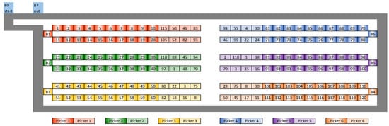
Figure 1. The layout of a distribution center where each picker is allocated to a single buffer: B0—start buffer; B7—out buffer; B1–B6—order picking buffers; Dark colors in buffers B1–B6—principal buffer products; light colors in buffers B1–B6—products also allocated in other buffers.

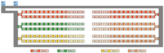
Figure 2. The layout of a distribution center where one picker is allocated to more than one buffer: B0—start buffer; B7—out buffer; B1–B6—order picking buffers; Dark colors in buffers B1–B6—principal buffer products; light colors in buffers B1–B6—products also allocated in other buffers.

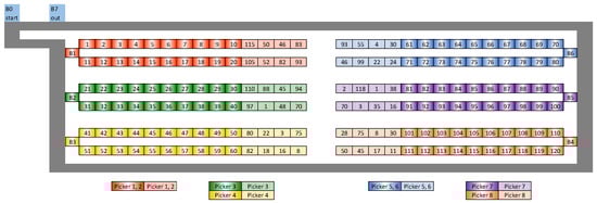
Figure 3. The layout of a distribution center where more than one picker is allocated to one buffer: B0—start buffer; B7—out buffer; B1–B6—order picking buffers; Dark colors in buffers B1–B6—principal buffer products; light colors in buffers B1–B6—products also allocated in other buffers.

Figure 1 shows one picker allocated to each buffer and one picker assigned to each buffer. In Figure 2, one picker is allocated to both buffers B4 and B5, making Picker 4 one of the multi-buffer pickers. In Figure 3, more than one picker is allocated to a single buffer; for example, pickers 1, 2, and 5, 6 are assigned to buffers B1 and B6, respectively.

In this research, we define the following main mathematical model.

Indices and sets:

$N$—number of orders;

$H$—number of products;

$R$—number of buffers;

$W$—number of pickers;

$i,m$—index for orders, $i,m=1,\dots ,N$;

$j,k$—index for products, $j,k=1,\dots ,H$;

$b,g$—index for buffers, $b,g=1,\dots ,R$;

$p,l$—index for pickers, $p=1,\dots ,W$.

Parameters:

$t_{ij}$—picking time of the product $j$ in the order $i$;

$s_b$—travel time from the depot to the buffer $b$;

$c_{ij}$—quantity of product $j$ in the order $i$ that must be picked by pickers;

$q_{bj}$—available quantity of the product $j$ in the buffer $b$;

$f_{bg}$—travel time from the buffer $b$ to the buffer $g$ (because the conveyor is one-directional, $f_{bg}\ne f_{gb}$);

$z_{bj}$—binary parameter of location products in buffers;

$z_{bj}=\left\{\begin{array}{l}1, \mathrm{if} \mathrm{the} \mathrm{product} j \mathrm{is} \mathrm{located} \\ \mathrm{in} \mathrm{the} \mathrm{buffer} b\\ 0, \mathrm{otherwise}\end{array}\right\}$;

$v_{pb}$—binary parameter of assignment pickers to buffers;

$v_{pb}=\left\{\begin{array}{l}1, \mathrm{if} \mathrm{the} \mathrm{picker} p \mathrm{is} \mathrm{assigned} \\ \mathrm{to} \mathrm{the} \mathrm{buffer} b\\ 0, \mathrm{otherwise}\end{array}\right\}$;

Decision variables in the main model:

$x_{ijpb}$—start time for the product $j$ in the order $i$ picked by the picker $p$ in the buffer $b$;

$y_{ijpb}$—quantity of the product $j$ in the order $i$ picked by the picker $p$ in the buffer $b$.

Decision variable in the step 1 matheuristics:

$y_{ijpb}$—quantity of the product $j$ in the order $i$ picked by the picker $p$ in the buffer $b$.

Decision expressions in the step 1 matheuristics:

$t_p^{pkr}$—processing time of the picker $p$;

$t_b^{bfr}$—occupied time of the buffer $b$.

Decision variable the step 2 matheuristics:

$x_{ijpb}$—start time for the product $j$ in the order $i$ picked by the picker $p$ in the buffer $b$;

Minimize the makespan:

$$\min \underset{i=1,\dots ,N}{\max }\underset{j=1,\dots ,H}{\max }\underset{p=1,\dots ,W}{\max }\underset{b=1,\dots ,R}{\max }(x_{ijpb}+t_{ij}),$$

(1)

Subject to:

Pickers to buffers assignment, i.e., the picker does not pick products in buffers to which the picker is not assigned.

$$\forall (p)\forall (i)\forall (j)\forall (b:v_{pb}=0)[y_{ijpb}=0],$$

(2)

Products to buffers assignment, i.e., picker does not pick products in buffers in which the product is not located.

$$\forall (p)\forall (i)\forall (j)\forall (b:z_{bj}=0)[y_{ijpb}=0],$$

(3)

Picking operations have precedence in each order, executed by all pickers in all buffers; i.e., the previous picking operation must finish before the start of any next picking operation for this order.

$$\begin{array}{l}\forall (i)\forall (j,k:j\ne k,t_{ij}\ne 0,t_{ik}\ne 0)[\underset{p=1,\dots ,W}{\max }\underset{b=1,\dots ,R}{\max }(x_{ijpb}+t_{ij})\le \underset{p=1,\dots ,W}{\min }\underset{b=1,\dots ,R}{\min }{x}_{ikpb}\vee \\ \vee \underset{p=1,\dots ,W}{\max }\underset{b=1,\dots ,R}{\max }(x_{ikpb}+t_{ik})\le \underset{p=1,\dots ,W}{\min }\underset{b=1,\dots ,R}{\min }{x}_{ijpb}]\end{array},$$

(4)

Each picker processes just one product for one order in all of his buffers at a time.

$$\forall (p)\forall (i,m:i\ne m)\forall (b:v_{pb}=1)\forall (j)[x_{ijpb}+t_{ij}\le x_{mjpb}\vee x_{mjpb}+t_{mj}\le x_{ijpb}],$$

(5)

Each picker in each order in all his buffers processes just one product at a time.

$$\forall (p)\forall (i)\forall (b:v_{pb}=1)\forall (j,k:j\ne k)[x_{ijpb}+t_{ij}\le x_{ikpb}\vee x_{ikpb}+t_{ik}\le x_{ijpb}],$$

(6)

Each picker in each order for all products processes products just at one of his buffers at a time.

$$\forall (p)\forall (i)\forall (j)\forall (b,g:b\ne g,v_{pb}=1,v_{pg}=1)[x_{ijpb}+t_{ij}\le x_{ijpg}\vee x_{ijpg}+t_{ij}\le x_{ijpb}],$$

(7)

Each picker at each of his buffers processes just one of the different orders and just one of the different products at a time.

$$\forall (p)\forall (b:v_{pb}=1)\forall (i,m:i\ne m)\forall (j,k:j\ne k)[x_{ijpb}+t_{ij}\le x_{mkpb}\vee x_{mkpb}+t_{mk}\le x_{ijpb}],$$

(8)

Each picker processes just one of the different orders, just one of the different products, and just one of his buffers at a time.

$$\begin{array}{l}\forall (p)\forall (b,g:b\ne g,v_{pb}=1,v_{pg}=1)\forall (i,m:i\ne m)\forall (j,k:j\ne k)\\ [x_{ijpb}+t_{ij}\le x_{mkpg}\vee x_{mkpg}+t_{mk}\le x_{ijpb}]\end{array},$$

(9)

The start of the picking operation at each buffer must occur no earlier than the travel time of the container to this buffer from the depot.

$$\forall (b)\forall (j:z_{bj}=1)\forall (i:t_{ij}\ne 0)\forall (p)[x_{ijpb}\ge z_{bj}{s}_b],$$

(10)

Travel time between buffers must be enough, i.e., we consider the travel time from buffer to buffer in one direction on the conveyor or a round trip beyond the depot to come to any of the previous buffers.

$$\begin{array}{l}\forall (i)\forall (j,k:j\ne k,t_{ij}\ne 0,t_{ik}\ne 0)\forall (b,g:b\ne g,z_{bj}=1,z_{gk}=1)\\ [\underset{p=1,\dots ,W}{\max }(x_{ijpb}+t_{ij})+r_{bg}\le \underset{p=1,\dots ,W}{\min }{x}_{ikpg}\vee \underset{p=1,\dots ,W}{\max }(x_{ikpg}+t_{ik})+r_{gb}\le \underset{p=1,\dots ,W}{\min }{x}_{ijpb}]\end{array},$$

(11)

Enough products are available at each buffer to be picked by all pickers for each order.

$$\forall (i)\forall (j)\forall (b)[{\displaystyle \sum _{p=1}^W{y}_{ijpb}}\le q_{bj}],$$

(12)

Enough products have been picked.

$$\forall (i)\forall (j)[{\displaystyle \sum _{p=1}^W{\displaystyle \sum _{b=1}^R{y}_{ijpb}}}=c_{ij}],$$

(13)

Each product is processed in one buffer by one picker.

$$\forall (i)\forall (j)\forall (p)[{\displaystyle \sum _{b=1}^R\min (y_{ijpb},1)}\le 1],$$

(14)

Decision variables:

Start time

$$x_{ijpb}=\{0,{\mathbb{\mathbb{Z}}}^{+}\},$$

(15)

Quantity

$$y_{ijpb}=\{0,{\mathbb{\mathbb{Z}}}^{+}\},$$

(16)

4. Matheuristics Development

Scheduling is a decision-making process in the real world of computing. Making a timetable is quite tricky due to resource constraints.

Heuristics are some rules to guide the search for a solution. Although they cannot promise to find the best solution, they can frequently find a workable one quickly. A heuristic is a method designed to solve a problem more quickly when more conventional methods are inefficient.

Matheuristics are optimization algorithms that are detached from the optimization problems and employ mathematical programming methods to produce heuristic solutions. Heuristic and matheuristic algorithms are typically simple to implement and quick to run, but they have the potential to miss better solutions or become stuck in local optima.

Both of the following methods of hybridization are possible: mathematical programming incorporated into heuristic and metaheuristic algorithms. The use of features derived from the mathematical model of optimization problems is a crucial component of some algorithms.

While commercial solvers work very well in some instances when solving scheduling problems, for others, they cannot find the optimal solution or any solution at all.

In this research, a mathematical programming-based technique was chosen since it would be challenging to develop a method that could produce high-quality solutions in a reasonable amount of time while taking into account all order-picking constraints derived from the distribution centers and warehouses. We propose to decompose the main order-picking problem into two subproblems and try to solve each of them using mathematical programming. The 1st step has two variants, such as the pickers’ free time minimization problem and the buffer s free time minimization problem, depending on the matheuristics number. Next, in the 2nd step, we solve the main order picking makespan minimization problem using input from step 1.

We develop two matheuristics, each of which consists of two steps described below (Figure 4).

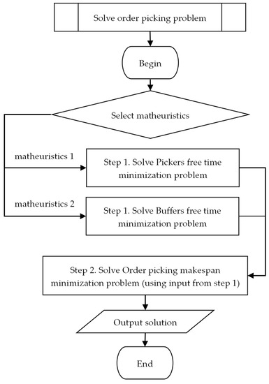
Figure 4. Procedure “Solve order picking problem”.

4.1. Step 1. Pickers (Buffers) Free Time Minimization Problem

In this research, we define the following additional decision expressions.

Decision expressions:

$$\begin{gathered} t_p^{pkr}={\displaystyle \sum _{i=1}^N{\displaystyle \sum _{j=1}^H{\displaystyle \sum _{b=1}^R\min (y_{ijpb},1)\cdot t_{ij}}}} \\ {t}_b^{bfr}={\displaystyle \sum _{i=1}^N{\displaystyle \sum _{j=1}^H{\displaystyle \sum _{p=1}^W\min (y_{ijpb},1)\cdot t_{ij}}}} \end{gathered}$$

Depending on the active matheuristics (Matheuristics 1 or Matheuristics 2), we define the two different criteria functions. The set of constraints is the same for each of the matheuristics. From the main model from Section 3, we take the constraints that steer the assignment of containers to pickers and buffers, excluding time sequencing constraints. Therefore, constraints (19) and (20) correspond to constraints (2) and (3), constraints (21)–(23) correspond to constraints (12)–(14). We define only the quantity decision variable (24) which corresponds to the decision variable (16).

Minimize the pickers’ free time if there is Matheuristics 1:

$$\min {\displaystyle \sum _{p=1}^W(\underset{l=1,\dots ,W}{\max }{t}_l^{pkr}-t_p^{pkr})},$$

(17)

Minimize the buffers’ free time if there is Matheuristics 2:

$$\min {\displaystyle \sum _{b=1}^R(\underset{g=1,\dots ,R}{\max }{t}_g^{bfr}-t_b^{bfr})},$$

(18)

Subject to:

Pickers to buffers assignment, i.e., the picker does not pick products in buffers to which the picker is not assigned.

$$\forall (p)\forall (i)\forall (j)\forall (b:v_{pb}=0)[y_{ijpb}=0],$$

(19)

Products to buffers assignment, i.e., the picker does not pick products in buffers in which the product is not located.

$$\forall (p)\forall (i)\forall (j)\forall (b:z_{bj}=0)[y_{ijpb}=0],$$

(20)

Enough products are available at each buffer to be picked by all pickers for each order.

$$\forall (i)\forall (j)\forall (b)[{\displaystyle \sum _{p=1}^W{y}_{ijpb}}\le q_{bj}],$$

(21)

Enough products have been picked.

$$\forall (i)\forall (j)[{\displaystyle \sum _{p=1}^W{\displaystyle \sum _{b=1}^R{y}_{ijpb}}}=c_{ij}],$$

(22)

Each product is processed in one buffer by one picker.

$$\forall (i)\forall (j)\forall (p)[{\displaystyle \sum _{b=1}^R\min (y_{ijpb},1)}\le 1],$$

(23)

Decision variable:

Quantity

$$y_{ijpb}=\{0,{\mathbb{\mathbb{Z}}}^{+}\},$$

(24)

4.2. Step 2. Order Picking Makespan Minimization Problem (Using $y_{ijpb}$ as Input from Step 1)

Using $y_{ijpb}$ as input from step 1, we define the following mathematical model. From the main model from Section 3, we take the time sequencing constraints. Therefore, constraints (26)–(33) correspond to constraints (4)–(11) from the full model. The goal function (25) corresponds to (1) from the full model. We define only the start time decision variable (34) which corresponds to the decision variable (15).

Minimize the makespan:

$$\min \underset{i=1,\dots ,N}{\max }\underset{j=1,\dots ,H}{\max }\underset{p=1,\dots ,W}{\max }\underset{b=1,\dots ,R}{\max }(x_{ijpb}+t_{ij}),$$

(25)

Subject to:

Picking operations have precedence in each order, executed by all pickers in all buffers; i.e., the previous picking operation must finish before the start of any next picking operation for this order.

$$\begin{array}{l}\forall (i)\forall (j,k:j\ne k,t_{ij}\ne 0,t_{ik}\ne 0)[\underset{p=1,\dots ,W}{\max }\underset{b=1,\dots ,R}{\max }(x_{ijpb}+t_{ij})\le \underset{p=1,\dots ,W}{\min }\underset{b=1,\dots ,R}{\min }{x}_{ikpb}\vee \\ \vee \underset{p=1,\dots ,W}{\max }\underset{b=1,\dots ,R}{\max }(x_{ikpb}+t_{ik})\le \underset{p=1,\dots ,W}{\min }\underset{b=1,\dots ,R}{\min }{x}_{ijpb}]\end{array},$$

(26)

Each picker processes just one product for one order in all of his buffers at a time.

$$\forall (p)\forall (i,m:i\ne m)\forall (b:v_{pb}=1)\forall (j)[x_{ijpb}+t_{ij}\le x_{mjpb}\vee x_{mjpb}+t_{mj}\le x_{ijpb}],$$

(27)

Each picker in each order in all his buffers processes just one product at a time.

$$\forall (p)\forall (i)\forall (b:v_{pb}=1)\forall (j,k:j\ne k)[x_{ijpb}+t_{ij}\le x_{ikpb}\vee x_{ikpb}+t_{ik}\le x_{ijpb}],$$

(28)

Each picker in each order for all products processes products just at one of his buffers at a time.

$$\forall (p)\forall (i)\forall (j)\forall (b,g:b\ne g,v_{pb}=1,v_{pg}=1)[x_{ijpb}+t_{ij}\le x_{ijpg}\vee x_{ijpg}+t_{ij}\le x_{ijpb}],$$

(29)

Each picker at each of his buffers processes just one of the different orders and just one of the different products at a time.

$$\forall (p)\forall (b:v_{pb}=1)\forall (i,m:i\ne m)\forall (j,k:j\ne k)[x_{ijpb}+t_{ij}\le x_{mkpb}\vee x_{mkpb}+t_{mk}\le x_{ijpb}],$$

(30)

Each picker processes just one of the different jobs, just one of the different products, and just one of his buffers at a time.

$$\begin{array}{l}\forall (p)\forall (b,g:b\ne g,v_{pb}=1,v_{pg}=1)\forall (i,m:i\ne m)\forall (j,k:j\ne k)\\ [x_{ijpb}+t_{ij}\le x_{mkpg}\vee x_{mkpg}+t_{mk}\le x_{ijpb}]\end{array},$$

(31)

The start of the picking operation at each buffer must occur no earlier than the travel time of the container to this buffer from the depot.

$$\forall (b)\forall (j:z_{bj}=1)\forall (i:t_{ij}\ne 0)\forall (p)[x_{ijpb}\ge z_{bj}{s}_b],$$

(32)

Travel time between buffers must be enough, i.e., we consider the travel time from buffer to buffer in one direction on the conveyor or a round trip beyond the depot to come to any of the previous buffers.

$$\begin{array}{l}\forall (i)\forall (j,k:j\ne k,t_{ij}\ne 0,t_{ik}\ne 0)\forall (b,g:b\ne g,z_{bj}=1,z_{gk}=1)\\ [\underset{p=1,\dots ,W}{\max }(x_{ijpb}+t_{ij})+r_{bg}\le \underset{p=1,\dots ,W}{\min }{x}_{ikpg}\vee \underset{p=1,\dots ,W}{\max }(x_{ikpg}+t_{ik})+r_{gb}\le \underset{p=1,\dots ,W}{\min }{x}_{ijpb}]\end{array},$$

(33)

Decision variable:

Start time

$$x_{ijpb}=\{0,{\mathbb{\mathbb{Z}}}^{+}\},$$

(34)

5. Experiment

The purpose of the computational experiment was to determine whether commercial tools like the CPLEX solver could be used to resolve the specified order-picking problem on instances of various sizes.

The experiments were performed using the solver version of IBM ILOG CPLEX Optimization Studio Version: 12.10.0.0

The computer parameters were:

• Processor: AMD Ryzen 5 1600 Six-Core Processor, 3.20 GHz
• System type: 64-bit operation system, x64-based processor
• RAM: 16 GB
• Operation system: Windows 10

In order to show the performance of the proposed algorithms, a test dataset was generated. Table 1 introduces the 120 test instances that were prepared for the experiment. One can find 10 instances of each of the distribution center layouts for each number of orders. There were 5, 10, 15, and 20 orders in each instance generated. The range of 1, …, five products were randomly generated to be picked into the container. There existed six, four, and eight pickers in the first, second, and third distribution center layouts consequently.

Table 1. Test data.

Instance	Orders	Distribution Centre Layout	Pickers	Locations	Repeated Locations	Buffers	Products in the Order
1–10	5	1	6	120	48	6	1, …, 5
11–20	10
21–30	15
31–40	20
41–50	5	2	4
51–60	10
61–70	15
71–80	20
81–90	5	3	8
91–100	10
101–110	15
111–120	20

Distribution center layouts are shown in Figure 1, Figure 2 and Figure 3. We generated 120 main and 48 repeated locations in the six buffers. The product was stored in one, two, or three locations in the distribution center. In total, 85 products were stored only in one location. A total of 22 products were stored in two locations. A total of 13 products were stored in three locations. The time limit for CPLEX execution was set at 5 min for each of the solving cases.

Table 2 reports the results of the matheuristics’ first step solution—pickers free time minimization problem—for five orders. The search was completed, and all instances were solved optimally. The number of solutions varied from one to three for the first layout (instances 1–10), from one to four for the second layout (instances 41–50), and from one to nine for the third layout (instances 81–90).

Table 2. Results for 2 steps matheuristics starting with solving pickers’ free time minimization problem for 5 orders.

	Step 1: Pickers’ Free Time Minimization Problem				Step 2: Order Picking Makespan Minimization Problem after Solving Pickers Free Time Minimization Problem
Instance	Number of Solutions	Time Spent in Solving [s]	Engine [s]	Extraction [s]	Number of Solutions	Comparison with the Lower Bound	Time Spent in Solving [s]	Engine [s]	Extraction [s]
1	2	2.54	0.96	1.58	7	42.19%	301.13	257.25	43.88
2	1	2.55	0.93	1.62	7	55.39%	302.81	258.31	44.49
3	1	2.50	0.84	1.65	4	40.79%	301.95	258.15	43.79
4	3	2.89	1.28	1.61	7	38.69%	302.39	258.56	43.82
5	2	2.81	1.18	1.63	6	36.46%	302.42	258.31	44.10
6	2	2.62	0.92	1.69	6	100.00%	301.23	256.85	44.38
7	1	2.45	0.84	1.60	1	0.00%	133.52	89.42	44.09
8	1	13.69	12.04	1.65	5	37.54%	300.80	256.74	44.05
9	3	2.59	0.98	1.60	4	6.97%	300.97	257.03	43.94
10	3	2.65	1.06	1.59	5	34.43%	300.71	256.40	44.31
41	4	2.29	1.40	0.89	7	66.93%	302.20	233.81	68.39
42	3	3.33	2.45	0.88	5	59.14%	303.28	234.80	68.47
43	1	2.93	2.03	0.89	4	58.19%	300.78	233.41	67.37
44	2	1.83	0.92	0.91	7	51.67%	302.31	234.92	67.38
45	2	6.71	5.81	0.90	5	53.30%	301.32	233.15	68.17
46	1	1.33	0.42	0.90	3	58.11%	302.16	232.77	69.39
47	2	1.49	0.62	0.87	6	51.36%	300.77	232.27	68.50
48	1	1.42	0.51	0.91	6	56.89%	301.42	235.52	65.89
49	1	5.68	4.78	0.89	5	60.52%	301.43	232.89	68.53
50	3	1.57	0.67	0.90	5	25.56%	300.82	232.14	68.67
81	2	35.96	33.32	2.64	2	100.00%	300.96	239.66	61.29
82	1	9.85	7.23	2.62	1	100.00%	303.26	243.07	60.18
83	1	32.56	29.92	2.64	2	39.51%	301.84	241.25	60.58
84	9	33.86	31.18	2.67	2	53.56%	302.32	241.95	60.36
85	3	4.50	1.88	2.62	2	54.93%	303.22	242.95	60.26
86	3	20.41	17.83	2.57	2	58.93%	303.33	243.30	60.02
87	4	23.06	20.42	2.63	1	43.04%	304.80	245.11	59.69
88	3	33.93	31.38	2.54	2	59.18%	304.85	244.59	60.26
89	2	14.95	12.40	2.55	1	61.70%	300.86	242.20	58.66
90	3	27.44	24.89	2.55	3	63.99%	302.42	241.78	60.64

The average time spent solving was 3.73 s and varied from 2.45 s to 13.69 s for the first layout (instances 1–10). The average time spent solving was 2.86 s and varied from 1.33 s to 6.71 s for the second layout (instances 41–50). The average time spent solving was 23.65 s and varied from 4.50 s to 35.96 s for the third layout (instances 81–90).

Table 2 also reports the results of the matheuristics’ second step solution—order picking makespan minimization problem after solving pickers free time minimization problem—for five orders. The search was completed only for the seventh instance, so only for this instance was an optimal solution found.

For 1–10 instances, the average gap to the lower bound was 39.25% and varied from 0.00% to 100.00%. In 41–50 instances, the average gap to the lower bound was 54.17% and varied from 25.56% to 66.93%. In 81–90 instances, the average gap to the lower bound was 63.48% and varied from 39.51% to 100.00%. The number of solutions varied from one to seven for the 1st layout (instances 1–10), from three to seven for the 2nd layout (instances 41–50), and from one to three for the third layout (instances 81–90).

The average time spent on solving was 284.79 s and varied from 133.52 s to 302.81 s for the first layout (instances 1–10). The average time spent on solving was 301.65 s and varied from 300.77 s to 303.28 s for the 2nd layout (instances 41–50). The average time spent solving was 302.79 s and varied from 300.86 s to 304.85 s for the 3rd layout (instances 81–90).

Table 3 reports the results of the matheuristics’ 1st step solution—the buffer free time minimization problem—for five orders. The search was completed, and all instances were solved optimally. The number of solutions varied from 1 to 3 for the first layout (instances 1–10), from 1 to 5 for the second layout (instances 41–50), and from 1 to 19 for the third layout (instances 81–90).

Table 3. Results for 2 steps matheuristics starting with solving buffers’ free time minimization problem for 5 orders.

	Step 1: Buffers’ Free Time Minimization Problem				Step 2: Order Picking Makespan Minimization Problem after Solving Buffers Free Time Minimization Problem
Instance	Number of Solutions	Time Spent in Solving [s]	Engine [s]	Extraction [s]	Number of Solutions	Comparison with the Lower Bound	Time Spent in Solving [s]	Engine [s]	Extraction [s]
1	2	2.62	0.99	1.63	7	42.19%	301.63	257.36	44.26
2	1	2.50	0.90	1.60	6	100.00%	300.36	254.73	45.63
3	1	2.49	0.84	1.65	3	43.28%	300.80	255.41	45.38
4	3	2.66	1.05	1.61	5	42.62%	301.70	255.23	46.46
5	2	2.89	1.21	1.68	5	36.99%	302.19	256.54	45.65
6	2	2.64	0.95	1.69	6	100.00%	302.61	257.98	44.62
7	2	2.57	0.87	1.70	1	0.00%	139.13	94.13	44.99
8	1	11.82	10.2	1.61	4	41.87%	301.41	256.50	44.91
9	3	2.63	1.02	1.61	6	6.97%	300.74	255.74	44.99
10	3	2.73	1.07	1.66	5	34.43%	301.66	256.98	44.68
41	5	2.40	1.27	1.13	7	66.93%	301.41	232.61	68.79
42	3	1.75	0.66	1.09	5	59.14%	301.99	234.89	67.09
43	2	1.89	0.75	1.13	4	58.19%	301.08	233.67	67.41
44	2	1.76	0.59	1.16	6	51.78%	302.36	234.86	67.49
45	5	2.01	0.86	1.14	5	53.30%	300.95	233.75	67.19
46	3	1.75	0.61	1.13	3	58.11%	300.95	232.82	68.13
47	2	1.92	0.77	1.15	7	51.26%	300.78	232.92	67.86
48	1	8.69	7.58	1.11	7	56.58%	301.11	234.20	66.90
49	2	1.84	0.69	1.14	5	60.52%	301.32	234.17	67.14
50	3	2.03	0.89	1.14	6	25.00%	301.16	232.14	69.02
81	2	27.85	25.73	2.12	2	100.00%	302.97	244.40	58.57
82	2	3.69	1.51	2.18	1	100.00%	301.63	242.83	58.79
83	5	4.65	2.44	2.20	2	39.51%	303.28	244.53	58.75
84	1	44.19	41.98	2.20	2	53.56%	302.57	244.50	58.06
85	2	3.97	1.78	2.18	2	54.93%	303.50	244.94	58.56
86	3	20.01	17.91	2.09	2	58.93%	304.08	242.37	61.70
87	4	3.98	1.82	2.15	1	43.04%	302.81	240.92	61.89
88	19	24.57	22.41	2.16	2	59.18%	304.38	243.28	61.10
89	2	3.41	1.32	2.08	1	61.70%	301.64	243.04	58.59
90	4	23.02	20.93	2.09	3	63.99%	301.17	242.12	59.05

The average time spent in solving was 3.56 s and varied from 2.49 s to 11.82 s for the 1st layout (instances 1–10). The average time spent solving was 2.60 s and varied from 1.75 s to 8.69 s for the second layout (instances 41–50). The average time spent solving was 15.93 s and varied from 3.41 s to 44.19 s for the third layout (instances 81–90).

Table 3 also reports the results of the matheuristics’ second step solution—order picking makespan minimization problem after solving buffers free time minimization problem—for five orders. The search was completed only for the seventh instance was so only for this instance was an optimal solution found.

For 1–10 instances, the average gap to the lower bound was 44.84% and varied from 0.00% to 100.00%. For 41–50 instances, the average gap to the lower bound was 54.08% and varied from 25.00% to 66.93%. For 81–90 instances, the average gap to the lower bound was 63.48% and varied from 39.51% to 100.00%. The number of solutions varied from one to seven for the first layout (instances 1–10), from three to seven for the second layout (instances 41–50), and from one to three for the third layout (instances 81–90).

The average time spent on solving was 285.22 s and varied from 139.13 s to 302.61 s for the 1st layout (instances 1–10). The average time spent on solving was 301.31 s and varied from 300.78 s to 302.36 s for the second layout (instances 41–50). The average time spent solving was 302.80 s and varied from 301.17 s to 304.38 s for the third layout (instances 81–90).

The results of the second step solution—order picking makespan minimization problem after solving buffers free time minimization problem—for five orders (Table 3) are very similar to the results of the 2nd step solution—order picking makespan minimization problem after solving pickers free time minimization problem—for 5 orders (Table 2) because a lot of the solutions found were the same. The differences between the results achieved by these two matheuristics are shown in Figure 5. Only different instances are presented in Figure 5.

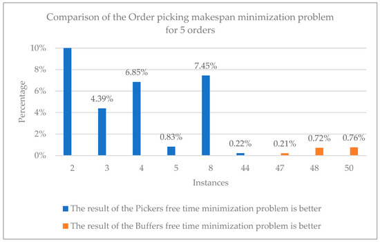
Figure 5. Comparison of the order picking makespan minimization problem after solving pickers free time minimization problem and buffers free time minimization problem for 5 orders.

The results of the matheuristics comparison show that the 1st matheuristics (pickers) was better than the 2nd matheuristics (puffers), having found six solutions that were better. The other matheuristics (buffers) found only 3 solutions that were better compared to the 1st matheuristics (pickers). Moreover, for the 2nd instance, the 1st matheuristics (pickers) found the solution, but the 2nd matheuristics (buffers) did not return any result (there is no signature on the column because the result is greater than 100%). Generally, the 1st matheuristics (pickers) found a better solution on average, not including the 2nd instance of 3.95%, but the 2nd matheuristics (buffers) found a better solution on average of only 0.56%.

Table 4 reports the results of the matheuristics’ 1st step solution—Pickers free time minimization problem—for 10 orders. The search was completed, and all instances were solved optimally. The number of solutions varied from 1 to 4 for the 1st layout (instances 11–20), from 1 to 6 for the 2nd layout (instances 51–60), and from 1 to 5 for the 3rd layout (instances 91–100).

Table 4. Step 1: Pickers and Buffers free time minimization problem for 10 orders.

	Step 1: Pickers’ Free Time Minimization Problem				Step 1: Buffers’ Free Time Minimization Problem
Instance	Number of Solutions	Time Spent in Solving [s]	Engine [s]	Extraction [s]	Number of Solutions	Time Spent in Solving [s]	Engine [s]	Extraction [s]
11	4	6.58	3.23	3.34	3	6.01	2.60	3.40
12	1	10.88	7.56	3.32	1	11.06	7.73	3.33
13	4	6.53	3.26	3.26	3	6.13	2.80	3.33
14	1	7.25	3.98	3.26	1	7.53	4.19	3.34
15	1	8.98	5.67	3.31	1	8.98	5.56	3.42
16	4	8.28	4.96	3.32	5	8.86	5.32	3.54
17	2	5.71	2.37	3.34	2	5.73	2.26	3.47
18	1	5.13	1.81	3.31	1	4.95	1.59	3.35
19	2	5.87	2.54	3.32	3	6.34	2.91	3.43
20	1	5.43	2.13	3.29	1	5.26	1.93	3.32
51	1	2.56	0.77	1.79	1	3.43	1.14	2.29
52	2	3.08	1.26	1.82	4	4.11	1.83	2.28
53	2	9.39	7.62	1.76	2	19.41	17.14	2.26
54	3	3.17	1.39	1.78	6	4.10	1.81	2.28
55	3	3.20	1.42	1.77	2	4.60	2.25	2.35
56	4	3.40	1.54	1.86	3	3.94	1.67	2.27
57	1	2.57	0.77	1.80	1	3.30	1.03	2.26
58	1	2.69	0.91	1.77	2	3.66	1.39	2.27
59	4	3.28	1.48	1.79	4	3.85	1.57	2.27
60	6	3.52	1.76	1.75	3	4.00	1.72	2.27
91	3	9.09	4.01	5.07	2	7.81	3.46	4.35
92	3	9.30	4.02	5.28	3	7.76	3.35	4.40
93	3	71.44	66.24	5.19	4	59.55	55.20	4.34
94	1	8.56	3.31	5.25	1	6.90	2.54	4.35
95	5	9.30	4.13	5.17	1	6.92	2.63	4.29
96	1	8.58	3.35	5.22	1	38.53	34.18	4.34
97	1	85.81	80.52	5.29	1	56.30	51.86	4.44
98	1	62.66	57.47	5.19	1	49.28	44.94	4.34
99	2	8.47	3.25	5.22	2	7.08	2.70	4.37
100	2	8.55	3.40	5.14	3	7.24	2.90	4.33

The average time spent on solving was 7.06 s and varied from 5.13 s to 10.88 s for the 1st layout (instances 11–20). The average time spent solving was 3.69 s and varied from 2.56 s to 9.39 s for the 2nd layout (instances 51–60). The average time spent solving was 28.18 s and varied from 8.47 s to 85.81 s for the 3rd layout (instances 91–100).

Table 4 also reports the results of the matheuristics’ 1st step solution—the buffer free time minimization problem—for 10 orders. The search was completed, and all instances were solved optimally. The number of solutions varied from 1 to 5 for the 1st layout (instances 11–20), from 1 to 6 for the 2nd layout (instances 51–60), and from 1 to 4 for the 3rd layout (instances 91–100).

The average time spent on solving was 7.09 s and varied from 4.95 s to 11.06 s for the 1st layout (instances 11–20). The average time spent on solving was 5.44 s and varied from 3.30 s to 19.41 s for the 2nd layout (instances 51–60). The average time spent solving was 24.74 s and varied from 6.90 s to 59.55 s for the 3rd layout (instances 91–100).

Table 5 reports the results of the matheuristics’ 1st step solution—pickers’ free time minimization problem—for 15 orders. The search was completed, and 21–30 and 61–70 instances were solved optimally. For the remaining 101–110 instances, the percentage comparison with the lower bound was calculated. For 101–110 instances, the average gap to the lower bound was 106.27% and varied from 18.57% to 305.70%. The number of solutions varied from 3 to 9 for the 1st layout (instances 21–30), from 2 to 15 for the 2nd layout (instances 61–70), and from 2 to 6 for the 3rd layout (instances 101–110).

Table 5. Step 1: Pickers’ and Buffers’ free time minimization problem for 15 orders.

	Step 1: Pickers’ Free Time Minimization Problem					Step 1: Buffers’ Free Time Minimization Problem
Instance	Number of Solutions	Comparison with the Lower Bound	Time Spent in Solving [s]	Engine [s]	Extraction [s]	Number of Solutions	Comparison with the Lower Bound	Time Spent in Solving [s]	Engine [s]	Extraction [s]
21	3	0.00%	9.53	4.63	4.90	5	0.00%	10.05	5.01	5.04
22	8	0.00%	70.96	66.01	4.94	8	0.00%	70.28	65.26	5.01
23	3	0.00%	63.24	58.29	4.94	4	0.00%	61.04	56.03	5.01
24	9	0.00%	67.71	56.58	5.12	6	0.00%	67.32	62.12	5.20
25	4	0.00%	10.02	5.07	4.94	5	0.00%	9.50	4.54	4.95
26	7	0.00%	10.49	5.52	4.97	11	0.00%	11.54	6.45	5.09
27	4	0.00%	68.95	63.95	4.99	5	0.00%	62.80	57.66	5.13
28	3	0.00%	111.35	106.41	4.94	4	0.00%	115.25	110.21	5.04
29	4	0.00%	53.67	48.61	5.05	3	0.00%	60.30	55.26	5.04
30	8	0.00%	59.40	54.48	4.91	13	0.00%	59.72	54.69	5.02
61	15	0.00%	109.96	107.22	2.73	18	0.00%	220.19	216.70	3.49
62	5	0.00%	29.18	26.54	2.64	9	0.00%	7.79	4.25	3.54
63	5	0.00%	35.44	32.75	2.69	3	0.00%	44.68	41.15	3.53
64	6	0.00%	38.71	35.98	2.72	12	0.00%	46.20	42.56	3.63
65	7	0.00%	5.84	3.11	2.72	4	0.00%	42.19	38.47	3.71
66	5	0.00%	40.22	37.54	2.68	6	0.00%	45.42	41.85	3.56
67	6	0.00%	33.20	30.45	2.74	2	0.00%	41.84	38.30	3.53
68	4	0.00%	34.56	31.82	2.73	3	0.00%	7.11	3.44	3.67
69	2	0.00%	22.91	20.20	2.71	2	0.00%	27.45	23.91	3.53
70	8	0.00%	34.24	31.51	2.73	3	0.00%	45.33	41.74	3.59
101	4	187.10%	300.20	292.16	8.04	7	528.60%	300.27	293.55	6.72
102	2	18.57%	300.20	292.50	7.69	3	34.19%	300.16	293.42	6.73
103	6	91.80%	300.19	292.33	7.86	4	206.00%	300.16	293.46	6.69
104	5	70.13%	300.24	291.97	8.27	5	558.10%	300.21	293.63	6.58
105	5	305.70%	300.26	292.44	7.82	9	716.50%	300.21	293.61	6.60
106	5	88.98%	300.33	292.52	7.80	2	80.20%	300.13	293.52	6.60
107	3	110.80%	300.22	292.46	7.76	3	237.90%	300.14	293.58	6.56
108	6	102.20%	300.23	292.21	8.01	6	102.20%	300.26	292.21	8.05
109	5	65.80%	300.34	292.31	8.03	7	186.40%	300.20	293.28	6.92
110	4	21.60%	300.26	292.27	7.98	3	49.62%	300.21	293.38	6.83

The average time spent in solving was 52.53 s and varied from 9.53 s to 111.35 s for the 1st layout (instances 21–30). The average time spent on solving was 38.43 s and varied from 5.84 s to 109.96 s for the 2nd layout (instances 61–70). The average time spent solving was 300.25 s and varied from 300.19 s to 300.34 s for the 3rd layout (instances 101–110).

Table 5 also reports the results of the matheuristics’ 1st step solution—the buffer free time minimization problem—for 15 orders. The search was completed, and 21–30 and 61–70 instances were solved optimally. For the remaining 101–110 instances, the percentage comparison with the lower bound was calculated. For 101–110 instances, the average gap to the lower bound was 269.97% and varied from 34.19% to 716.50%. The number of solutions varied from 3 to 13 for the 1st layout (instances 21–30), from 2 to 18 for the 2nd layout (instances 61–70), and from 2 to 9 for the 3rd layout (instances 101–110).

The average time spent in solving was 52.78 s and varied from 9.50 s to 115.25 s for the 1st layout (instances 21–30). The average time spent on solving was 52.82 s and varied from 7.11 s to 200.19 s for the 2nd layout (instances 61–70). The average time spent solving was 300.20 s and varied from 300.13 s to 300.27 s for the 3rd layout (instances 101–110).

Table 6 reports the results of the matheuristics’ 1st step solution—pickers’ free time minimization problem—for 20 orders. The search was completed for eight instances of the 1st layout and for all instances of the 2nd layout. They were solved optimally. For the rest of the instances, the percentage comparison with the lower bound was calculated. For 111–120 instances, the average gap to the lower bound was 786.91% and varied from 33.78% to 6306.00%. The number of solutions varied from 2 to 15 for the 1st layout (instances 31–40), from 1 to 15 for the 2nd layout (instances 71–80), and from 1 to 18 for the 3rd layout (instances 111–120).

Table 6. Step 1: Pickers’ and Buffers’ free time minimization problem for 20 orders.

	Step 1: Pickers’ Free Time Minimization Problem					Step 1: Buffers’ Free Time Minimization Problem
Instance	Number of Solutions	Comparison with the Lower Bound	Time Spent in Solving [s]	Engine [s]	Extraction [s]	Number of Solutions	Comparison with the Lower Bound	Time Spent in Solving [s]	Engine [s]	Extraction [s]
31	2	0.00%	109.4	102.70	6.69	3	0.00%	116.64	109.86	6.77
32	5	0.00%	95.68	89.18	6.50	5	0.00%	96.10	89.35	6.74
33	11	0.00%	116.38	109.80	6.57	7	0.00%	108.37	101.64	6.72
34	3	0.00%	97.50	90.87	6.63	4	0.00%	93.97	87.13	6.84
35	15	0.00%	99.68	92.80	6.88	9	0.00%	105.61	98.78	6.82
36	9	0.00%	14.07	7.48	6.58	7	0.00%	16.14	9.14	7.00
37	15	0.00%	104.58	97.86	6.72	12	0.00%	102.55	95.75	6.80
38	5	0.00%	116.49	109.91	6.58	12	0.00%	119.88	113.24	6.63
39	4	44.07%	300.14	293.49	6.64	3	44.07%	300.20	293.41	6.78
40	6	49.85%	300.18	293.59	6.58	3	44.48%	300.18	293.21	6.96
71	12	0.00%	56.96	53.26	3.70	8	0.00%	62.34	57.50	4.84
72	3	0.00%	6.36	2.70	3.66	4	0.00%	8.35	3.61	4.73
73	1	0.00%	70.63	66.98	3.64	1	0.00%	79.91	75.16	4.75
74	10	0.00%	69.66	66.07	3.59	14	0.00%	104.96	100.32	4.63
75	2	0.00%	48.76	45.13	3.62	1	0.00%	51.33	46.66	4.67
76	6	0.00%	52.96	49.34	3.62	3	0.00%	63.11	58.47	4.63
77	4	0.00%	42.93	39.23	3.69	6	0.00%	11.32	6.49	4.83
78	15	0.00%	60.95	57.33	3.62	13	0.00%	76.11	71.44	4.67
79	3	0.00%	107.29	103.69	3.60	4	0.00%	92.86	88.01	4.85
80	3	0.00%	8.44	4.79	3.64	5	0.00%	53.92	49.21	4.70
111	6	201.40%	300.38	289.58	10.80	14	1472.00%	300.29	291.52	8.77
112	5	126.90%	301.16	290.68	10.48	5	540.20%	300.23	291.43	8.80
113	3	208.50%	300.34	289.78	10.56	17	669.10%	300.46	291.43	9.03
114	5	100.10%	300.28	289.71	10.57	6	190.50%	300.27	291.44	8.82
115	10	133.90%	300.38	289.55	10.82	8	538.70%	300.33	291.40	8.93
116	2	33.78%	300.35	289.76	10.59	4	174.00%	300.23	291.34	8.88
117	9	591.10%	300.35	289.70	10.65	10	3147.00%	300.28	291.38	8.90
118	18	6306.00%	300.35	289.70	10.65	15	1436.00%	300.33	291.52	8.81
119	1	45.54%	300.32	289.34	10.97	3	81.56%	300.33	291.51	8.82
120	9	121.90%	300.26	289.65	10.60	8	362.70%	300.60	291.84	8.76

The average time spent on solving was 135.41 s and varied from 14.07 s to 300.18 s for the 1st layout (instances 31–40). The average time spent solving was 52.49 s and varied from 6.36 s to 107.29 s for the 2nd layout (instances 71–80). The average time spent solving was 300.42 s and varied from 300.26 s to 301.16 s for the 3rd layout (instances 111–120).

Table 6 also reports the results of the matheuristics’ 1st step solution—the buffer free time minimization problem—for 20 orders. The search was completed for eight instances of the 1st layout and for all instances of the 2nd layout. They were solved optimally. For the remaining instances, the percentage comparison with the lower bound was calculated. For 111–120 instances, the average gap to the lower bound was 861.18% and varied from 81.56% to 3147.00%. The number of solutions varied from 3 to 12 for the 1st layout (instances 31–40), from 1 to 14 for the 2nd layout (instances 71–80), and from 3 to 17 for the 3rd layout (instances 111–120).

The average time spent on solving was 135.96 s and varied from 16.14 s to 300.20 s for the 1st layout (instances 31–40). The average time spent on solving was 60.42 s and varied from 8.35 s to 104.96 s for the 2nd layout (instances 71–80). The average time spent solving was 300.34 s and varied from 300.23 s to 300.60 s for the 3rd layout (instances 111–120).

The outcomes show that the proposed order picking makespan minimization problem for five orders could be solved by the CPLEX solver. In the 1st step, both matheuristics (pickers and buffers free time minimization problems) found optimal solutions for all 30 instances, but in the 2nd step, only 1 optimal solution from 30 instances was obtained.

For 10 orders, only the first step was solved by both matheuristics, which also found optimal solutions for all 30 instances. For 15 orders in the 1st step, both matheuristics could find optimal solutions for 2 out of 30 instances for the 1st and 2nd layouts only. For 20 orders in the 1st step, both matheuristics could find optimal solutions for 8 out of 10 instances for the 1st layout and for all 10 instances for the 2nd layout. For the remaining 10 instances of the 3rd layout, feasible solutions were obtained. Despite the problem decomposition, it was not possible for the CPLEX solver to solve the 2nd step of both matheuristics for 10, 15, or 20 orders. The 3rd layout, where more than one picker was assigned to one buffer, was the most difficult to solve. Therefore, for wholesalers, if the order includes a large variety of different products, the proposed mathematical programming is not appropriate, and more advanced heuristics are required.

Managing orders in the distribution centers and warehouses means finding ways to improve order-picking activities that allow the pickers to have a better work experience.

6. Conclusions

With the help of warehouse management systems, distributors can utilize the power of innovation to eliminate waste, boost order accuracy, cut operational expenses, and provide high levels of service.

The heuristics are broad guidelines you can use to make technological products that are easier to use, more readily available, and more intuitive. The best heuristics are developed by practitioners, who incorporate their years of professional experience, insights, and skills.

In this research, the order-picking problem is formulated as a mixed integer program (MIP); next, we solve it using a commercial solver. As for medium and large instances, MIP solvers cannot always provide an optimal or even any solution in a limited time, and we propose a method of how the order picking problem could be decomposed for solving it using the optimizer, for example, the CPLEX solver.

Also, through our numerical experiments, we gain some managerial knowledge. Appropriate decision-making in warehouses and distribution centers enhances the effectiveness of order-picking operations as a whole. At the cost of a slight increase in operating expenditures, it is possible to improve employee well-being and loyalty.

The experiment confirms that the proposed matheuristics can solve the proposed order picking makespan minimization problem for five orders with good enough results.

Despite the fact that all instances for 10 orders were solved optimally by the first step of both matheuristics (pickers and buffers free time minimization problems), the solution of the 2nd step of both matheuristics could not be obtained by the CPLEX solver as it was out of memory and returned the error “Opl process is not responding”. A similar situation occurred with 15 and 20 orders. This means that the proposed approach of decomposing the main problem into two subproblems and trying to solve each of them separately is suitable for small instances that are very frequently encountered in distribution centers and warehouses. This is the most frequent case in the distribution center. Therefore, the proposed matheuristics are very useful.

For large instances, more sophisticated heuristics are required. The solution from the first step of both matheuristics (pickers and buffers free time minimization problems) could be used as the initial part of future heuristics. Next, the newly developed matheuristics could improve assignment orders to pickers in buffers by re-arranging them.

Obviously, each sale and shipping type involves a different approach to the organization of the distribution center and warehouse, as well as economic and technological activities. When the products are sold directly to consumers with a small amount of product variety in the order, the developed matheuristics can improve decision-making, allow for better operations, and lower costs through digital transformation.

The proposed matheuristics could be part of the warehouse management solutions that are made to help the supply chain reach its full strategic potential so the distributors can obtain a competitive edge.

The obvious prospective area of future study is how to enhance the heuristic. Regarding that, we have one recommendation. With the help of an effective 1st step of both matheuristics (pickers and buffers for free time minimization problems), the performance of the next parts of heuristics can be improved. This proposition also includes the methods of simplifying and reformulating constraints in order to make the 1st step of both matheuristics be solved optimally or near optimally for large instances. Further improvement should also include hybridization methods, for example, the combination of mathematical programming with heuristic and metaheuristic algorithms. Such an approach could enhance well-known mathematical programming methods.

References

- Diefenbach, H.; Emde, S.; Glock, C.H.; Grosse, E.H. New Solution Procedures for the Order Picker Routing Problem in U-Shaped Pick Areas with a Movable Depot. OR Spectr. 2022, 44, 535–573. [Google Scholar] [CrossRef]
- van Gils, T.; Ramaekers, K.; Caris, A.; de Koster, R.B.M. Designing Efficient Order Picking Systems by Combining Planning Problems: State-of-the-Art Classification and Review. Eur. J. Oper. Res. 2018, 267, 1–15. [Google Scholar] [CrossRef]
- Grosse, E.H.; Glock, C.H.; Jaber, M.Y.; Neumann, W.P. Incorporating Human Factors in Order Picking Planning Models: Framework and Research Opportunities. Int. J. Prod. Res. 2015, 53, 695–717. [Google Scholar] [CrossRef]
- de Koster, R.; Le-Duc, T.; Roodbergen, K.J. Design and Control of Warehouse Order Picking: A Literature Review. Eur. J. Oper. Res. 2007, 182, 481–501. [Google Scholar] [CrossRef]
- Guo, X.; He, Y. Mathematical Modeling and Optimization of Platform Service Supply Chains: A Literature Review. Mathematics 2022, 10, 4307. [Google Scholar] [CrossRef]
- Song, M.; Fisher, R.; de Sousa Jabbour, A.B.L.; Santibañez Gonzalez, E.D.R. Green and Sustainable Supply Chain Management in the Platform Economy. Int. J. Logist. Res. Appl. 2022, 25, 349–363. [Google Scholar] [CrossRef]
- Georgijevic, M.; Bojic, S.; Brcanov, D. The Location of Public Logistic Centers: An Expanded Capacity-Limited Fixed Cost Location-Allocation Modeling Approach. Transp. Plan. Technol. 2013, 36, 218–229. [Google Scholar] [CrossRef]
- Fedorko, G.; Molnár, V.; Mikušová, N. The Use of a Simulation Model for High-Runner Strategy Implementation in Warehouse Logistics. Sustainability 2020, 12, 9818. [Google Scholar] [CrossRef]
- Nechi, S.; Aouni, B.; Mrabet, Z. Managing Sustainable Development through Goal Programming Model and Satisfaction Functions. Ann. Oper. Res. 2020, 293, 747–766. [Google Scholar] [CrossRef]
- Govindan, K.; Agarwal, V.; Darbari, J.D.; Jha, P.C. An Integrated Decision Making Model for the Selection of Sustainable Forward and Reverse Logistic Providers. Ann. Oper. Res. 2019, 273, 607–650. [Google Scholar] [CrossRef]
- Wulfert, T.; Woroch, R.; Strobel, G.; Seufert, S.; Möller, F. Developing Design Principles to Standardize E-Commerce Ecosystems: A Systematic Literature Review and Multi-Case Study of Boundary Resources. Electron. Mark. 2022, 32, 1813–1842. [Google Scholar] [CrossRef]
- Ali, S.S.; Kaur, R.; Khan, S. Evaluating Sustainability Initiatives in Warehouse for Measuring Sustainability Performance: An Emerging Economy Perspective. Ann. Oper. Res. 2023, 324, 461–500. [Google Scholar] [CrossRef]
- Chiang, T.A.; Che, Z.H.; Hung, C.W. A K-Means Clustering and the Prim’s Minimum Spanning Tree-Based Optimal Picking-List Consolidation and Assignment Methodology for Achieving the Sustainable Warehouse Operations. Sustainability 2023, 15, 3544. [Google Scholar] [CrossRef]
- Ries, J.M.; Grosse, E.H.; Fichtinger, J. Environmental Impact of Warehousing: A Scenario Analysis for the United States. Int. J. Prod. Res. 2017, 55, 6485–6499. [Google Scholar] [CrossRef]
- Du, S.; Hu, L.; Wang, L. Low-Carbon Supply Policies and Supply Chain Performance with Carbon Concerned Demand. Ann. Oper. Res. 2017, 255, 569–590. [Google Scholar] [CrossRef]
- Den Berg, J.P.V.; Zijm, W.H.M. Models for Warehouse Management: Classification and Examples. Int. J. Prod. Econ. 1999, 59, 519–528. [Google Scholar] [CrossRef]
- Staudt, F.H.; Alpan, G.; Di Mascolo, M.; Rodriguez, C.M.T. Warehouse Performance Measurement: A Literature Review. Int. J. Prod. Res. 2015, 53, 5524–5544. [Google Scholar] [CrossRef]
- Revillot-Narváez, D.; Pérez-Galarce, F.; Álvarez-Miranda, E. Optimising the Storage Assignment and Order-Picking for the Compact Drive-in Storage System. Int. J. Prod. Res. 2020, 58, 6949–6969. [Google Scholar] [CrossRef]
- Islam, M.R.; Ali, S.M.; Fathollahi-Fard, A.M.; Kabir, G. A Novel Particle Swarm Optimization-Based Grey Model for the Prediction of Warehouse Performance. J. Comput. Des. Eng. 2021, 8, 705–727. [Google Scholar] [CrossRef]
- Baruffaldi, G.; Accorsi, R.; Manzini, R. Warehouse Management System Customization and Information Availability in 3pl Companies: A Decision-Support Tool. Ind. Manag. Data Syst. 2019, 119, 251–273. [Google Scholar] [CrossRef]
- Diefenbach, H.; Glock, C.H. Ergonomic and Economic Optimization of Layout and Item Assignment of a U-Shaped Order Picking Zone. Comput. Ind. Eng. 2019, 138, 106094. [Google Scholar] [CrossRef]
- Masae, M.; Glock, C.H.; Grosse, E.H. Order Picker Routing in Warehouses: A Systematic Literature Review. Int. J. Prod. Econ. 2020, 224, 107564. [Google Scholar] [CrossRef]
- Bozer, Y.A.; Aldarondo, F.J. A Simulation-Based Comparison of Two Goods-to-Person Order Picking Systems in an Online Retail Setting. Int. J. Prod. Res. 2018, 56, 3838–3858. [Google Scholar] [CrossRef]
- Bormann, R.; de Brito, B.F.; Lindermayr, J.; Omainska, M.; Patel, M. Towards Automated Order Picking Robots for Warehouses and Retail. In Computer Vision Systems, Proceedings of the 12th International Conference, ICVS 2019, Thessaloniki, Greece, 23–25 September 2019; Lecture Notes in Computer Science (LNCS); Springer: Berlin/Heidelberg, Germany, 2019; Volume 11754, pp. 185–198. [Google Scholar]
- Boysen, N.; Stephan, K.; Weidinger, F. Manual Order Consolidation with Put Walls: The Batched Order Bin Sequencing Problem. EURO J. Transp. Logist. 2019, 8, 169–193. [Google Scholar] [CrossRef]
- Klumpp, M.; Loske, D. Order Picking and E-Commerce: Introducing Non-Parametric Efficiency Measurement for Sustainable Retail Logistics. J. Theor. Appl. Electron. Commer. Res. 2021, 16, 846–858. [Google Scholar] [CrossRef]
- Pérez-Rodríguez, R.; Hernández-Aguirre, A.; Jöns, S. A Continuous Estimation of Distribution Algorithm for the Online Order-Batching Problem. Int. J. Adv. Manuf. Technol. 2015, 79, 569–588. [Google Scholar] [CrossRef]
- Le-Duc, T.; de Koster, R.M.B.M. Travel Time Estimation and Order Batching in a 2-Block Warehouse. Eur. J. Oper. Res. 2007, 176, 374–388. [Google Scholar] [CrossRef]
- Vazquez-Noguerol, M.; Comesaña-Benavides, J.; Poler, R.; Prado-Prado, J.C. An Optimisation Approach for the E-Grocery Order Picking and Delivery Problem. Cent. Eur. J. Oper. Res. 2022, 30, 961–990. [Google Scholar] [CrossRef]
- Moons, S.; Ramaekers, K.; Caris, A.; Arda, Y. Integration of Order Picking and Vehicle Routing in a B2C E-Commerce Context. Flex. Serv. Manuf. J. 2018, 30, 813–843. [Google Scholar] [CrossRef]
- Pietri, N.O.; Chou, X.; Loske, D.; Klumpp, M.; Montemanni, R. The Buy-Online-Pick-up-in-Store Retailing Model: Optimization Strategies for in-Store Picking and Packing. Algorithms 2021, 14, 350. [Google Scholar] [CrossRef]
- Murfield, M.; Boone, C.A.; Rutner, P.; Thomas, R. Investigating Logistics Service Quality in Omni-Channel Retailing. Int. J. Phys. Distrib. Logist. Manag. 2017, 47, 263–296. [Google Scholar] [CrossRef]
- Boyer, K.K.; Hult, G.T.; Frohlich, M. An Exploratory Analysis of Extended Grocery Supply Chain Operations and Home Delivery. Integr. Manuf. Syst. 2003, 14, 652–663. [Google Scholar] [CrossRef]
- Huang, M.; Guo, Q.; Liu, J.; Huang, X. Mixed Model Assembly Line Scheduling Approach to Order Picking Problem in Online Supermarkets. Sustainability 2018, 10, 3931. [Google Scholar] [CrossRef]
- Öncan, T. A Genetic Algorithm for the order batching problem in low-level picker-to-part warehouse systems. In Proceedings of the International MultiConference of Engineers and Computer Scientists 2013, IMECS 2013, Hong Kong, 13–15 March 2013. [Google Scholar]
- Haouassi, M.; Kergosien, Y.; Mendoza, J.E.; Rousseau, L.M. The Integrated Orderline Batching, Batch Scheduling, and Picker Routing Problem with Multiple Pickers: The Benefits of Splitting Customer Orders. Flex. Serv. Manuf. J. 2022, 34, 614–645. [Google Scholar] [CrossRef]
- Manzini, R.; Gamberi, M.; Regattieri, A. Design and Control of a Flexible Order-Picking System (FOPS) a New Integrated Approach to the Implementation of an Expert System. J. Manuf. Technol. Manag. 2005, 16, 18–35. [Google Scholar] [CrossRef]
- Manzini, R.; Gamberi, M.; Persona, A.; Regattieri, A. Design of a Class Based Storage Picker to Product Order Picking System. Int. J. Adv. Manuf. Technol. 2007, 32, 811–821. [Google Scholar] [CrossRef]
- Yu, M.; de Koster, R.B.M. The Impact of Order Batching and Picking Area Zoning on Order Picking System Performance. Eur. J. Oper. Res. 2009, 198, 480–490. [Google Scholar] [CrossRef]
Disclaimer/Publisher’s Note: The statements, opinions and data contained in all publications are solely those of the individual author(s) and contributor(s) and not of MDPI and/or the editor(s). MDPI and/or the editor(s) disclaim responsibility for any injury to people or property resulting from any ideas, methods, instructions or products referred to in the content. |
© 2023 by the authors. Licensee MDPI, Basel, Switzerland. This article is an open access article distributed under the terms and conditions of the Creative Commons Attribution (CC BY) license (https://creativecommons.org/licenses/by/4.0/).