Development of a 7-DOF Biodynamic Model for a Seated Human and a Hybrid Optimization Method for Estimating Human-Seat Interaction Parameters

Abstract

Existing biodynamic models adopt apparent mass and seat-to-head transmissibility to predict the response of seated humans to whole-body vibration, limiting their ability to capture the actual response of distinct body segments in different excitation conditions. This study systematically develops a 7-DOF seated human model, a vibration experiment, and a novel hybrid optimization to estimate unknown mechanical parameters and predict the response of different human body segments to vertical vibrations. Experimental results showed that the upper trunk and head were most susceptible to transmitted vibrations. Combining the 7-DOF model and HOM resulted in accelerated optimization, improved numerical stability, and significant minimization of the objective function value compared to conventional algorithms. Notably, the estimated parameters, particularly stiffness, remained consistent regardless of increasing excitation magnitude or change in the body segment data used. Additionally, the model captured the non-linearity in human biodynamics through stiffness softening. These findings are applicable in seating systems optimization for comfort and safety.

1. Introduction

The study of the effects of whole-body vibration (WBV) on human health is a topic of significant interest, particularly due to the increased exposure of individuals to whole-body vibration resulting from vehicular transport. Prolonged exposure to WBV can lead to discomfort and adversely affect the health of passengers, particularly in a constrained sitting posture [1,2]. In this regard, it is essential to investigate how vibration is transmitted to the human body, especially in seated posture.

The region of the resonant frequency of vibration that affects passengers is of critical importance. The effect of WBV on the seated human body is more dominant under low-frequency excitation, specifically below 30 Hz [3]. Several studies have reported the principal resonant frequencies within less than 13 Hz, with the dominant peak in the frequency range of 4–6 Hz under vertical vibrations [4,5,6]. Therefore, studying the effects of vertical vibrations in regions within 0–15 Hz on different body segments is important to design systems that ensure that the human natural frequencies do not coincide with excitation frequency within this range.

One effective technique for investigating the dynamic response of humans to WBV is the development and use of biodynamic seated human models with different postural and excitation conditions. Biodynamic models are used to augment experimental measurements, which are not only time-consuming but limited by safety considerations. Existing biodynamic models are primarily categorized into finite element (FE), multibody (MB), and lumped parameter (LP) models. While complex models like finite elements and multibody systems may provide a more detailed representation of human body dynamics, a lumped-parameter model can be sufficient for investigating the dynamic response of humans to vibration. The simplicity and computational efficiency of lumped-parameter models make them ideal for exploring different scenarios and investigating the effects of different parameters on the system’s response [6]. Furthermore, lumped-parameter models have been extensively validated against experimental data and can be customized to include more detailed features of the human body, making them a viable option for investigating the dynamic response of humans to vibration [7,8,9,10].

The estimation of appropriate human parameters using biodynamics models is another widely reported issue in WBV studies. It is highly difficult to measure human mechanical parameters such as stiffness and damping coefficient from live tissues. Likewise, seats are made from viscoelastic materials whose mechanical properties are also difficult to measure [9,11,12]. Therefore, researchers estimate these viscoelastic properties through the minimization of errors between the biodynamic model responses and a target response function derived from the measured responses from experiments. Most existing studies consider measured vertical apparent mass (AM) as a target response function due to the rapid convergence of the AM optimization problem. A few studies also adopted seat-to-head transmissibility (STHT) in the parameter’s optimization problem [6,8]. However, model parameter identification with AM does not often describe the contributions of low inertia upper body segments to the total response [13]. Studies by Cho and Yoon [8] and Matsumo and Griffin [14] established that transmissibility is more appropriate for predicting transmitted vibration to selected body segments. Therefore, it is necessary to directly measure the response of each body segment to whole-body vibration in order to access the distinct response of the body segments to vibration, and so far, there are limited studies in this area.

Existing studies adopt either gradient-based or evolutionary-based algorithms to estimate the parameters of biodynamic models. However, there is still an exhaustive search for the appropriate optimization method that produces reliable estimates of these human parameters. For instance, Bae and Kang, Shao et al., and Huang et al. (2020) [10,15,16] optimized the parameters of 2-, 3-, 4-, and 5-DOF models using the gradient-based MATLAB function, called “fmincon”. Zhang et al. [17] introduced a reference vector-guided evolutionary algorithm to obtain the parameters of a 7-DOF human model, whereas Zhao et al. [18] explored multi-objective and genetic algorithms (GAs) for parameter identification of a 5-DOF model. From these studies, it was found that the separate or hybrid application of these optimization techniques is usually associated with trade-offs that include an exhaustive search for initial values, randomly generated optimal solutions, high computation time, and generation of estimated parameters that do not reflect the dynamic response of the human body to WBV [6,19]. Therefore, there is still a gap in research to develop model parameter estimation algorithms that are both reliable and computationally efficient.

In this study, we developed a lumped parameter seven-degree-of-freedom (7-DOF) biodynamic model for a seated human under vertical vibrations, including rotational degrees-of-freedom (DOF) and seat (and backrest) modeled as massless torsional and translational spring and damper. We designed a vibration experiment to obtain the transmissibility of different body segments of a seated subject under random base excitation in the vertical direction. A new hybrid optimization method (HOM) that combines gradient-based and genetic algorithms in some systematically defined steps was developed to estimate unknown stiffness and damping parameters of the model. We quantitatively evaluate the model fitting performances of the optimization methods using goodness-of-fit criteria, objective function value at the final solution, and computation speed. The sensitivities of the estimated parameters to the appearance and magnitude of the resonance frequencies were studied based on the relationship between the increment of the excitation magnitudes (0.5 to 2.0 m/s² rms) and using the transmissibility of different body segments in the optimization problem. Important findings on the key parameters affecting the region of resonance and how vibration is transmitted to each body segment were discussed. Ultimately, the development of the 7-DOF biodynamic model and HOM advances research on the optimization of comfort and safety for individuals when riding in vehicles.

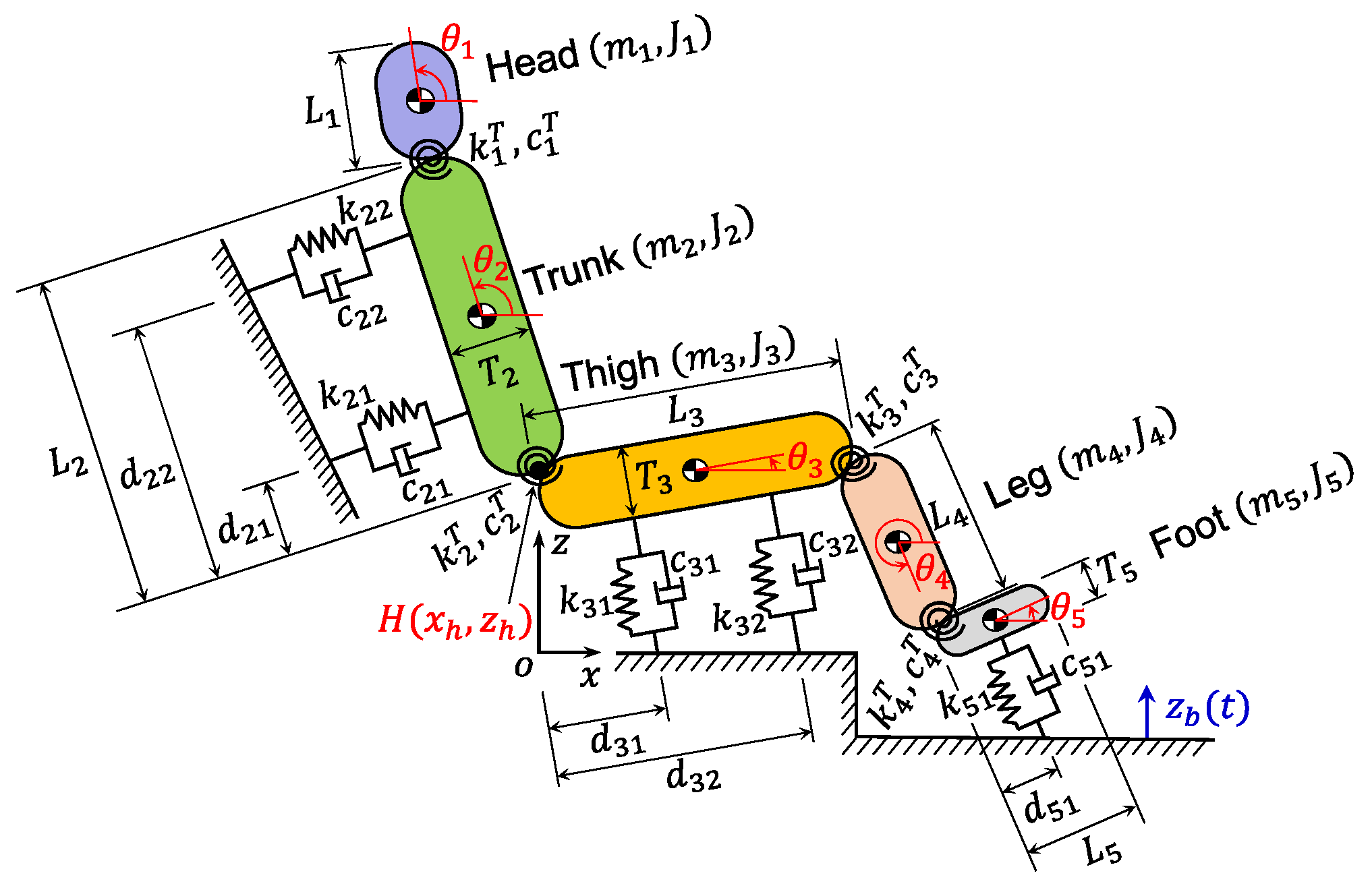
2. Development of the 7-DOF Human Model

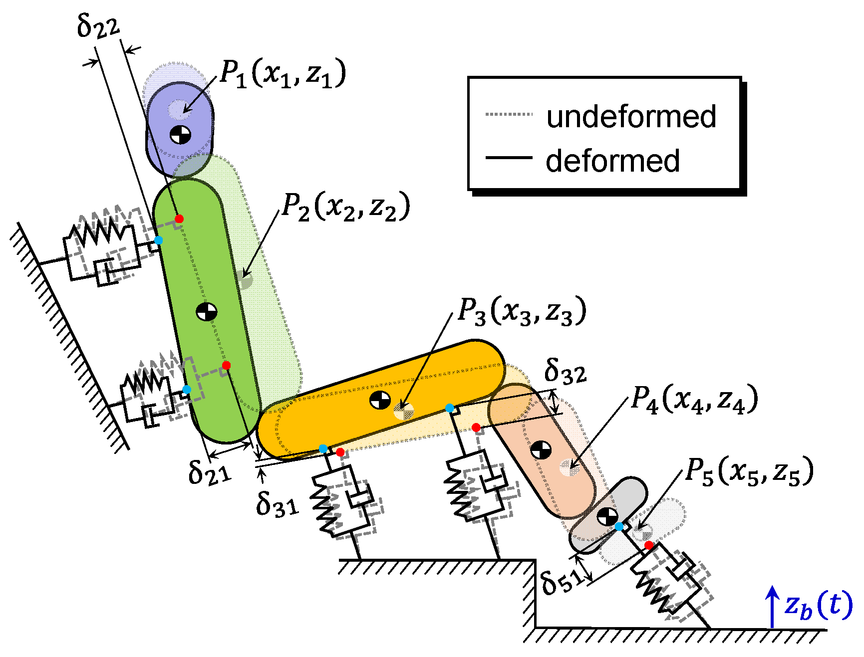
2.1. Model Description

The proposed 7-DOF biodynamic model consists of lumped parameters, including mass, spring, and damper elements. The model considers distinct body segments, comprising the upper body parts (including the head, neck, trunk, and upper extremities) and the lower body parts (including the pelvis, thigh, knee, leg, ankle, and foot). Each segment is treated as nonoverlapping, with the center of mass identified close to the proximal joints. The transmission of vibration from the seat to other segments is influenced by the viscoelastic properties of the human-seat coupling. Viscoelastic seats exhibit higher resonance frequencies compared to rigid seats [12,20]. To account for this, we represent the human-seat coupling using effective translational spring-damper combinations attached to the trunk and thigh, mimicking the viscoelastic properties of human skin and seat foam. The coupling between the shoe, foot skin, and foot segment is also modeled as an effective translational spring damper. These spring-damper combinations are attached perpendicularly to their respective body segments. Additionally, the joints at the hip, neck, knee, and ankle are modeled as torsional spring-damper elements, allowing rotation in the x-z plane.

Figure 1 illustrates the 7-DOF seated human model, consisting of five rigid bodies connected by dynamic joints and supported by a backrest. The model is subjected to vertical excitation, with $m_1$, $m_2$, $m_3$, $m_4$, $m_5$ representing the mass and $J_1$, $J_2$, $J_3$, $J_4$, $J_5$ representing the moment of inertia of the head, trunk, thigh, leg, and foot, respectively. The lengths of the segments are denoted as $L_1$, $L_2$, $L_3$, $L_4$, $L_5$, and the trunk, thigh, and foot have thicknesses $T_2$, $T_3$, $T_5.$ The translational spring-damper elements attached to the trunk, thigh, and foot are characterized by stiffness coefficients $k_{21}$, $k_{22}$, $k_{31}$, $k_{32}$, $k_{51}$ and damping coefficients $c_{21}$, $c_{22}$, $c_{31}$, $c_{32}$, $c_{51}$. The distances between the joints and the spring-damper combinations on trunk, thigh, and foot are represented by $d_{21}$, $d_{22}$, $d_{31}$, $d_{32,}$ and $d_{51}$. The torsional spring-damper elements at the joints have stiffness coefficients $k_1^T$, $k_2^T$, $k_3^T$, $k_4^T$ and damping coefficients $c_1^T$, $c_2^T$, $c_3^T$, $c_4^T$ and $z_b$ is the seat base excitation.

2.2. Derivation of Model Equations of Motion

The equations governing motions in the 7-DOF human model were derived through the Lagrangian dynamics approach in the form:

$$\frac{d}{dt}\left(\frac{\partial \left(KE\right)}{\partial {\dot{q}}_k}\right)-\frac{\partial \left(KE\right)}{\partial q_k}+\frac{\partial \left(PE\right)}{\partial q_k}+\frac{\partial D}{\partial {\dot{q}}_k}=0\left(k=1, 2,\cdots ,7\right)$$

(1)

where $q_k=\left\{x_h,z_h,{\theta }_1,{\theta }_2,{\theta }_3,{\theta }_4,{\theta }_5\right\}$ are the generalized coordinates corresponding to the horizontal and vertical displacement of the hip joint and rotational displacement of the center of gravity of each body segment of the 7-DOF model.

The kinetic energy (KE) of the system is given as:

$$KE=\frac{1}{2}\sum _{i=1}^5{m}_i\left({\dot{x}}_i^2+{\dot{z}}_i^2\right)+\frac{1}{2}\sum _{i=1}^5{J}_i{\dot{\theta }}_i^2,$$

(2)

where $x_i$ and $z_i$ are the position vectors of the center of gravity of the body segments in the x–z plane derived as

$$x_1=x_h+\frac{L_1}{2}\cos {\theta }_1+L_2\cos {\theta }_2, x_2=x_h+\frac{L_2}{2}\cos {\theta }_2,$$

$$x_3=x_h+\frac{L_3}{2}\cos {\theta }_3, x_4=x_h+L_3\cos {\theta }_3+\frac{L_4}{2}\cos {\theta }_4$$

(3)

$$x_5=x_h+L_3\cos {\theta }_3+L_4\cos {\theta }_4+\frac{L_5}{2}\cos {\theta }_5,$$

$$z_1=z_h+\frac{L_1}{2}\sin {\theta }_1+L_2\sin {\theta }_2, z_2=z_h+\frac{L_2}{2}\sin {\theta }_2,$$

$$z_3=z_h+\frac{L_3}{2}\sin {\theta }_3, z_4=z_h+L_3\sin {\theta }_3+\frac{L_4}{2}\sin {\theta }_4,$$

(4)

$$z_5=z_h+L_3\sin {\theta }_3+L_4\sin {\theta }_4+\frac{L_5}{2}\sin {\theta }_5$$

Equations of the potential energy (PE) and Rayleigh’s dissipation function (D) of the system are given as:

$$PE=\frac{1}{2}\sum _{i=2,j=1}^5{k}_{ij}{\delta }_{ij}^2+\frac{1}{2}\sum _{i=1}^4{k}_i^T{\varphi }_i^2+\sum _{i=1}^5{m}_{i}g\left({∆z}_i\right),$$

(5)

$$D=\frac{1}{2}\sum _{i=2,j=1}^5{c}_{ij}{\dot{\delta }}_{ij}^2+\frac{1}{2}\sum _{i=1}^5{c}_i^T{\dot{\varphi }}_i^2,$$

(6)

where ${\delta }_{ij}$ and ${\varphi }_i$ are the deflections of the translational and torsional springs; g represents gravity; and ${∆z}_i$ is the change in the value of z-axis position vector of the center of gravity of body segments.

The deformation of the 7-DOF model under the influence of the vertical excitation, $z_b$ is presented in Figure 2. The deflection terms, ${\delta }_{ij}$ and ${\varphi }_i$ are taken as the displacement of the position of the translational and torsional spring-damper as the model vibrates from the undeformed to the deformed configurations. Similarly, the position of the center of gravity, $P_i$ with coordinates, $x_i$ and $z_i$ during vibrations is considered. The deflection of the torsional spring damper, ${\varphi }_i$ is derived as the angular deflection during vibrations in the form:

$${\varphi }_1=\left({\theta }_1-{\theta }_1^{\mathrm{*}}\right)-\left({\theta }_2-{\theta }_2^{\mathrm{*}}\right), {\varphi }_2=\left({\theta }_2-{\theta }_2^{\mathrm{*}}\right)-\left({\theta }_3-{\theta }_3^{\mathrm{*}}\right),$$

$${\varphi }_3=\left({\theta }_4-{\theta }_4^{\mathrm{*}}\right)-\left({\theta }_3-{\theta }_3^{\mathrm{*}}\right), {\varphi }_4=\left({\theta }_5-{\theta }_5^{\mathrm{*}}\right)-\left({\theta }_4-{\theta }_4^{\mathrm{*}}\right),$$

(7)

where * denotes the initial value of the angle before vibration. On the other hand, the deflection of the translational spring-damper, ${\delta }_{ij}$ is taken as the parallel displacement of the ends of the translational spring-damper with respect to the undeformed configuration. The coordinates of the ends of the spring damper are derived by setting the hip joint as the reference point.

For instance, the derivation of deflection of the spring-damper at the thigh segment is described in Figure 3a. The position of the hip joint before and after deformation is denoted as $C_{31}^{\mathrm{*}}\left(x_h^{\mathrm{*}},z_h^{\mathrm{*}}\right)$ and $C_{31}\left(x_h,z_h\right)$; $B_{31}^{\mathrm{*}}$ and $B_{32}^{\mathrm{*}}$ are the position of the end of the first and second spring-damper in the undeformed configuration and $B_{31}$ and $B_{32}$ in the deformed configuration attached to the thigh; $A_{31}^{\mathrm{*}}$ and $A_{32}^{\mathrm{*}}$, are the fixed ends of the spring-damper; ${∆}_{31}^{\mathrm{*}}$ and ${∆}_{32}^{\mathrm{*}}$, are the unstretched length of the first and second spring-damper. The asterisk * represent the undeformed state for each of these points. Considering the first spring damper in Figure 3a, ${\delta }_{31}$ is the parallel spring extension from ${\mathit{B}}_{31}^{\mathrm{*}}{\mathit{A}}_{31}^{\mathrm{*}}$ to ${\mathit{B}}_{31}{\mathit{A}}_{31}^{\mathrm{*}}$ with respect to the undeformed configuration, where x–z coordinates for points, $A_{31}^{\mathrm{*}}\left(x_{31}^{\mathrm{*}},z_{31}^{\mathrm{*}}\right)$ and $B_{31}\left(x_{31},z_{31}\right)$ are derived as

$$x_{31}^{\mathrm{*}}=x_h^{\mathrm{*}}+\frac{T_3}{2}\sin {\theta }_3^{\mathrm{*}}+d_{31}\cos {\theta }_3^{\mathrm{*}}+{∆}_{31}^{\mathrm{*}}\sin {\theta }_3^{\mathrm{*}},$$

(8)

$$z_{31}^{\mathrm{*}}=z_h^{\mathrm{*}}-\frac{T_3}{2}\cos {\theta }_3^{\mathrm{*}}+d_{31}\sin {\theta }_3^{\mathrm{*}}-{∆}_{31}^{\mathrm{*}}\cos {\theta }_3^{\mathrm{*}},$$

(9)

$$x_{31}=x_h+\frac{T_3}{2}\sin {\theta }_3+d_{31}\cos {\theta }_3,$$

(10)

$$z_{31}=z_h-\frac{T_3}{2}\cos {\theta }_3+d_{31}\sin {\theta }_3+z_b$$

(11)

and by rotating the thigh through ${\theta }_3^{\mathrm{*}}$, we can see that ${\delta }_{31}$ is the vertical axis (z-axis) displacement of the spring. Clockwise rotation transformation is applied to ${\mathit{B}}_{31}{\mathit{A}}_{31}^{\mathrm{*}}$ in the form

$${\left[\begin{array}{c}{x}_{31}-x_{31}^{\mathrm{*}}\\ z_{31}-z_{31}^{\mathrm{*}}\end{array}\right]}^{\mathrm{\prime }}=\left[\begin{array}{cc}\cos {\theta }_3^{\mathrm{*}}& \sin {\theta }_3^{\mathrm{*}}\\ -\sin {\theta }_3^{\mathrm{*}}& \cos {\theta }_3^{\mathrm{*}}\end{array}\right]\left[\begin{array}{c}{x}_{31}-x_{31}^{\mathrm{*}}\\ z_{31}-z_{31}^{\mathrm{*}}\end{array}\right]$$

(12)

where prime represents transformed terms of ${\mathit{B}}_{31}{\mathit{A}}_{31}^{\mathrm{*}}$. The transformed vertical axis displacement is thus derived as

$$\begin{array}{l}{\delta }_{31}=-\left(x_{31}-x_{31}^{\mathrm{*}}\right)\sin {\theta }_3^{\mathrm{*}}+\left(z_{31}-z_{31}^{\mathrm{*}}\right)\cos {\theta }_3^{\mathrm{*}}-{\mathsf{\Delta }}_{31}^{\mathrm{*}}\\ \hspace{1em}=\left(z_h-z_h^{\mathrm{*}}\right)\cos {\theta }_3^{\mathrm{*}}-\left(x_h-x_h^{\mathrm{*}}\right)\sin {\theta }_3^{\mathrm{*}}-\frac{T_3}{2}\cos \left({\theta }_3-{\theta }_3^{\mathrm{*}}\right)+d_{31}\sin \left({\theta }_3-{\theta }_3^{\mathrm{*}}\right)\\ \hspace{1em}\hspace{1em}\hspace{1em}\hspace{1em}\hspace{1em}\hspace{1em}\hspace{1em}\hspace{1em}\hspace{1em}+\frac{T_3}{2}+z_b\cos {\theta }_3^{\mathrm{*}}\end{array}$$

(13)

The transformation matrix technique was applied to derive an expression for ${\delta }_{32}$ such that all terms in Equation (13) were retained except $d_{31}$ that changed to $d_{32}$. A transformation rotation through ${\theta }_5^{\mathrm{*}}$ was applied to the foot region, as shown in Figure 3b. The expressions for coordinates of the points, $A_{51}^{\mathrm{*}}\left(x_{51}^{\mathrm{*}},z_{51}^{\mathrm{*}}\right)$ and $B_{51}\left(x_{51},z_{51}\right)$ applied in the derivation of ${\delta }_{51}$ are as follows:

$$x_{51}^{\mathrm{*}}=x_h^{\mathrm{*}}+\frac{T_3}{2}\sin {\theta }_3^{\mathrm{*}}+L_3\cos {\theta }_3^{\mathrm{*}}+L_4\cos {\theta }_4^{\mathrm{*}}+\frac{T_5}{2}\sin {\theta }_5^{\mathrm{*}}+d_{51}\cos {\theta }_5^{\mathrm{*}}+{∆}_{51}^{\mathrm{*}}\sin {\theta }_5^{\mathrm{*}},$$

(14)

$$z_{51}^{\mathrm{*}}=z_h^{\mathrm{*}}-\frac{T_3}{2}\cos {\theta }_3^{\mathrm{*}}+L_3\sin {\theta }_3^{\mathrm{*}}-L_4\sin {\theta }_4^{\mathrm{*}}-\frac{T_5}{2}\cos {\theta }_5^{\mathrm{*}}+d_{51}\sin {\theta }_5^{\mathrm{*}}-{∆}_{51}^{\mathrm{*}}\cos {\theta }_5^{\mathrm{*}},$$

(15)

$$x_{51}=x_h+\frac{T_3}{2}\sin {\theta }_3+L_3\cos {\theta }_3+L_4\cos {\theta }_4+\frac{T_5}{2}\sin {\theta }_5+d_{51}\cos {\theta }_5,$$

(16)

$$z_{51}=z_h-\frac{T_3}{2}\cos {\theta }_3+L_3\sin {\theta }_3-L_4\sin {\theta }_4-\frac{T_5}{2}\cos {\theta }_5+d_{51}\sin {\theta }_5+z_b\left(t\right)$$

(17)

In contrast, we applied counterclockwise rotation to the trunk region through $\left(\pi -{\theta }_2^{\mathrm{*}}\right)$, as shown in Figure 3c. The expressions for coordinates of the points, $A_{21}^{\mathrm{*}}\left(x_{21}^{\mathrm{*}},z_{21}^{\mathrm{*}}\right)$ and $B_{21}\left(x_{21},z_{21}\right)$ applied in the derivation of ${\delta }_{21}$ are as follows:

$$x_{21}^{\mathrm{*}}=x_h^{\mathrm{*}}-\frac{T_2}{2}\sin {\theta }_2^{\mathrm{*}}-d_{21}\cos {\theta }_2^{\mathrm{*}}-{∆}_{21}^{\mathrm{*}}\sin {\theta }_2^{\mathrm{*}},$$

(18)

$$z_{21}^{\mathrm{*}}=z_h^{\mathrm{*}}+\frac{T_2}{2}\cos {\theta }_2^{\mathrm{*}}+d_{21}\sin {\theta }_2^{\mathrm{*}}+{∆}_{21}^{\mathrm{*}}\cos {\theta }_2^{\mathrm{*}},$$

(19)

$$x_{21}=x_h-\frac{T_2}{2}\sin {\theta }_2+d_{21}\cos {\theta }_2,$$

(20)

$$z_{21}=z_h+\frac{T_2}{2}\cos {\theta }_2+d_{21}\sin {\theta }_2+z_b\left(t\right),$$

(21)

The coordinates of the points, $A_{22}^{\mathrm{*}}\left(x_{22}^{\mathrm{*}},z_{22}^{\mathrm{*}}\right)$ and $B_{22}\left(x_{22},z_{22}\right)$ were obtained such that all terms in Equations (18)–(21) were retained except for the length terms $d_{21}$ and ${∆}_{21}^{\mathrm{*}}$, which changed to $d_{22}$ and ${∆}_{22}^{\mathrm{*}}$, respectively. Substituting the expressions in Equations (3), (4), and (7) and expressions for ${\delta }_{11}$, ${\delta }_{12}$, ${\delta }_{21}$, ${\delta }_{22}$ and ${\delta }_{51}$, into the energy equations in (2), (5), and (6), we solve Lagrange’s equation in (1) and obtained non-linear equations of motion with respect to each generalized coordinate, $q_k$. The expressions for the deflection terms ${\delta }_{21}$, ${\delta }_{22}$, ${\delta }_{32,}$ and ${\delta }_{51}$ are provided in Appendix A.

2.3. Linearization of Equations of Motion

Non-linear analysis of a vibrating system is not only complex, difficult, and time-consuming, but it also challenges access to familiar modal properties, such as natural frequencies and mode shapes. Therefore, we employed linearization techniques on the 7-DOF model’s non-linear equations of motion by expanding the Taylor’s series at the initial configurations using the following approximations:

$$\theta ={\theta }^{\mathrm{*}}+\tilde{\theta },\cos \tilde{\theta }=1,\sin \tilde{\theta }=\tilde{\theta },$$

(22)

where $\tilde{\theta }$ is a small perturbation around the initial value of absolute angular deflection, ${\theta }^{\mathrm{*}}$.

The linearized equations of motion, expressed as a matrix, are written in the form:

$$\mathbf{M}\ddot{\mathit{x}}\left(t\right)+\mathbf{C}\dot{\mathit{x}}\left(t\right)+\mathbf{K}\mathit{x}\left(t\right)={\mathit{f}}_{\mathit{c}}{\dot{z}}_b\left(t\right)+{\mathit{f}}_{\mathit{k}}{z}_b\left(t\right),$$

(23)

where $\mathbf{M}$, $\mathbf{C},$ and $\mathbf{K}$ are mass, damping, and stiffness matrices; $\mathit{x}\left(t\right)$ is the generalized coordinates vector; ${\mathit{f}}_{\mathit{k}}$ and ${\mathit{f}}_{\mathit{c}}$ are generalized stiffness and damping coefficients vectors; $z_b\left(t\right)$ is displacement due to input excitation. Taking the Fourier transform of Equation (23), the linear equations of motion in the frequency domain are expressed as:

$$\mathit{X}\left(j\omega \right)={\left(-{\omega }^2\mathbf{M}+j\omega \mathbf{C}+\mathbf{K}\right)}^{-1}\left(j\omega {\mathit{f}}_{\mathit{c}}+{\mathit{f}}_{\mathit{k}}\right)Z_b\left(j\omega \right)$$

(24)

The transmissibility from the seat to each segment of the 7-DOF model can be computed from Equation (24) and will be used in the estimation of the unknown parameters. The expressions for the matrices and force vectors are provided in Appendix B.

3. Human Vibration Experiment and Identification of Human Parameters

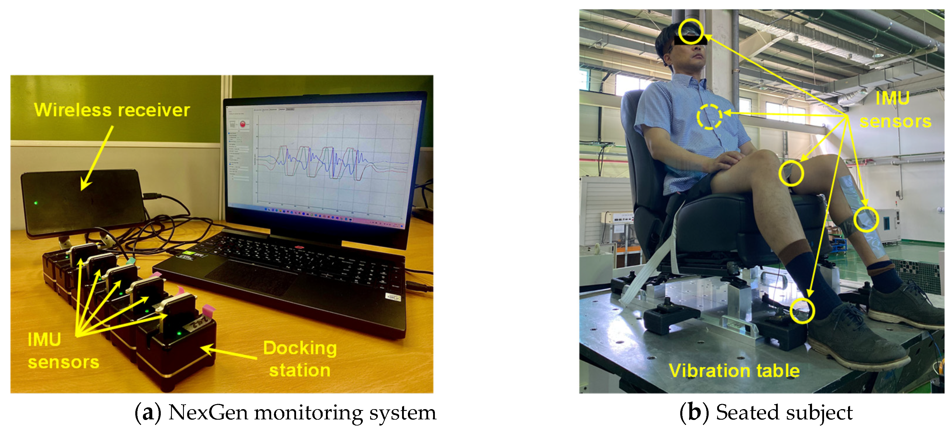
3.1. Experimental Set-Up and Procedures

We conducted a human vibration experiment at the Jeonbuk Institute of Automotive Technology (JIAT) to measure the dynamic response of a seated human to vertical vibrations using an MTS 248.05 uniaxial hydraulic exciter (Figure 4a). The subject sat on a viscoelastic vehicle seat (Figure 4b), fixed tightly to the vibration table using an aluminum test jig. Random vibration within the excitation frequency range of 2–80 Hz was applied to the subject in the vertical direction. The acceleration of the body segments of the subject under vertical vibrations was recorded using a NexGen monitoring system (Figure 5a), which comprises a wireless receiver, docking station, TK Motion Manager software (eZ-Analyst V5.1.140), and SXT movement monitors (inertial measurement unit, IMU sensors). During the vibration measurement, the IMU sensors were tightly fixed to the skin of the subject at the head, thigh, leg, chest (under the cloth), and at the base of the seat (Figure 5b). The IMU sensors had a sampling frequency of 128 Hz, and vertical excitations of 0.5 and 2.0 m/s² rms were applied for 5 min per session.

Afterward, the measured acceleration signals were processed using MATLAB signal processing techniques. We applied a Hanning window with 50% overlap and 19 averages and computed the transmissibility from the base to each body segment using the ‘modalfrf’ function in MATLAB. The technical specifications of the uniaxial hydraulic exciter are listed in

Table 1. Specifications of the uniaxial exciter used in the experiment.

Model	Max. Dynamic Force	Max. Displacement	Operating Frequency	Vibration Table
MTS 248.05 Hydraulic	±50 kN	75 mm	0.1~100 Hz	1.2 × 1.2 m

.

3.2. Identification of Human Parameters

For physical modeling, simulation, or parameter estimation, physical properties such as mass, mass moment of inertia, length, and thickness of body segments are required [21]. We extracted the mass, length, and thickness of human body segments from the 8th Korean Human Body Dimension Survey Report of Size Korea [22], which provided data for Korean adult males and females aged 18–59 years, with an average height of 171 cm and weight of 70 kg, within the range of body size of the subject used in our experiment. The corresponding mass moment of inertia data was reported by Ma et al. [23], who used a 3D scan to calculate the moment of inertia of various human segments. Also, we obtained the range of initial angles of the body segments in a seated posture from Kim et al. [24] and adapted the appropriate angles to the 7-DOF model. The identified human and geometric parameters used in the 7-DOF model equations of motion are listed in

Table 2. Identified human and geometric parameters.

Mass (kg)		Moment of Inertia (kg·m2)		Length (m)		Thickness (m)		Initial Angle (deg.)		Spring Ends Distance (m)
$m_1$	5.66	$J_1$	0.037	$L_1$	0.263			${\theta }_1$	100	$d_1$	0.100
$m_2$	37.96	$J_2$	2.050	$L_2$	0.599	$T_2$	0.224	${\theta }_2$	111	$d_2$	0.479
$m_3$	18.74	$J_3$	0.324	$L_3$	0.495	$T_3$	0.156	${\theta }_3$	12	$d_3$	0.088
$m_4$	6.08	$J_4$	0.061	$L_4$	0.368			${\theta }_4$	306	$d_4$	0.459
$m_5$	1.56	$J_5$	0.005	$L_5$	0.248	$T_5$	0.076	${\theta }_5$	10	$d_5$	0.124

.

4. Optimization Methods

4.1. Objective Function Formulation

We developed an objective function to estimate the unknown stiffness and damping parameters by minimizing the sum of squared errors between measured and calculated transmissibility:

$$Minimize\hspace{1em}\frac{{\int }_{f_1}^{f_2}{\left|T_{Exp.}\left(f\right)-T_{Model}\left(f\right)\right|}^{2}df}{{\int }_{f_1}^{f_2}{\left|T_{Exp.}\left(f\right)\right|}^{2}df}$$

(25)

$$Subject to\hspace{1em}20\le k_{ij}\le 200 kN/m, and 1 \le k_i^T\le 4 kNm/rad$$

$$\hspace{1em}\hspace{1em}\hspace{1em}\hspace{1em}\hspace{1em}10\le c_{ij}\le 4000 Ns/m, and 5\le c_i^T\le 500 Nms/rad$$

where $T_{Exp.}$ and $T_{Model}$ are transmissibility obtained from experiments and those calculated using Equation (24) for each body segment, while $f_{\mathrm{1,2}}$ is the frequency range of vibration measurements. For our analysis, $T_{Exp.}$ measured at the head, trunk, thigh, and leg were used as feeding data in the objective function to estimate the unknown stiffness and damping parameters. The parameters were subject to upper and lower bounds obtained from reviewing the published range of values of stiffness and damping in the literature [15,16,25,26,27]. The specified bounds limit the estimated stiffness and damping coefficients to only positive values and speed up the convergence of the optimization algorithms.

4.2. Gradient-Based Algorithm (GBA)

Gradient-based algorithms (GBAs) are commonly used in human model parameter estimation due to their speed and ease of implementation. However, they have some limitations, such as being highly sensitive to the initial values of the unknown parameters. This limitation becomes even more significant in a study like ours where there are no established data on the values of stiffness and damping coefficients that can accurately model the viscoelastic properties of the skin and seat subject to dynamic excitations.

In this study, we execute GBA using the ‘fmincon’ MATLAB optimization function to minimize the sum of squared errors between measured and calculated transmissibility in the 7-DOF model. We initially set computation parameters, including a maximum iteration of 50, a step tolerance of 1 × 10⁻¹⁵, and a function tolerance of 1 × 10⁻¹², under the bounds specified in Equation (25). However, this resulted in a poor fitting of the transmissibility and high objective function value at final solutions. The objective function value at final solutions (FVAL) is a real number returned when the algorithm converges. Typically, in a minimization problem, the lower the FVAL, the higher the chances that the obtained solution is close to the optimum solution of the desired problem [28].

To improve the fitting results by GBA, we continuously adjusted the computation parameters using trial-and-error techniques. Finally, we achieved much better fits, with an FVAL of 0.0513 obtained at the final solutions of GBA using an average of 100 iterations, a maximum function evaluation of 2700, and within the computation time of 1300 s. The difficulties in finding the appropriate initial values demonstrate the challenges associated with GBA in estimating human parameters and highlight the importance of carefully selecting and adjusting the computation parameters to obtain accurate and reliable solutions.

4.3. Genetic Algorithm (GA)

Unlike gradient-based algorithms, genetic algorithm (GA) is a gradient-free optimization technique that is used to find global or near-global optima without specifying initial values. The algorithm is based on a random population evolution technique using some set of operators. In this study, we employed GA to estimate stiffness and damping values while fitting the measured and calculated transmissibility. GA was executed using the ‘ga’ function in MATLAB with a population size of 90, 9 elites, crossover probability of 0.8, function tolerance of 1 × 10⁻¹², 100 maximum generations, adaptive feasible mutation function, and defaults values for the creation, fitness scaling, selection, and crossover functions. At this time, the algorithm obtained poor fitting of the transmissibility plots with a mean FVAL of 0.1078 returned after 880 s.

According to Mathworks [28], a larger population size improves the capability of GA to comprehensively search for optimal values close to the global optima, albeit at the expense of the computation speed. The initial population size was increased to 180 and then 270, while other computation parameters were retained, resulting in much-improved fits of the transmissibility plots as presented in Section 5.

However, the optimized parameters obtained by GA were characterized by high instability, making it difficult to perform parameter sensitivity analyses on the optimized stiffness and damping coefficients’ dynamic response to the excitation.

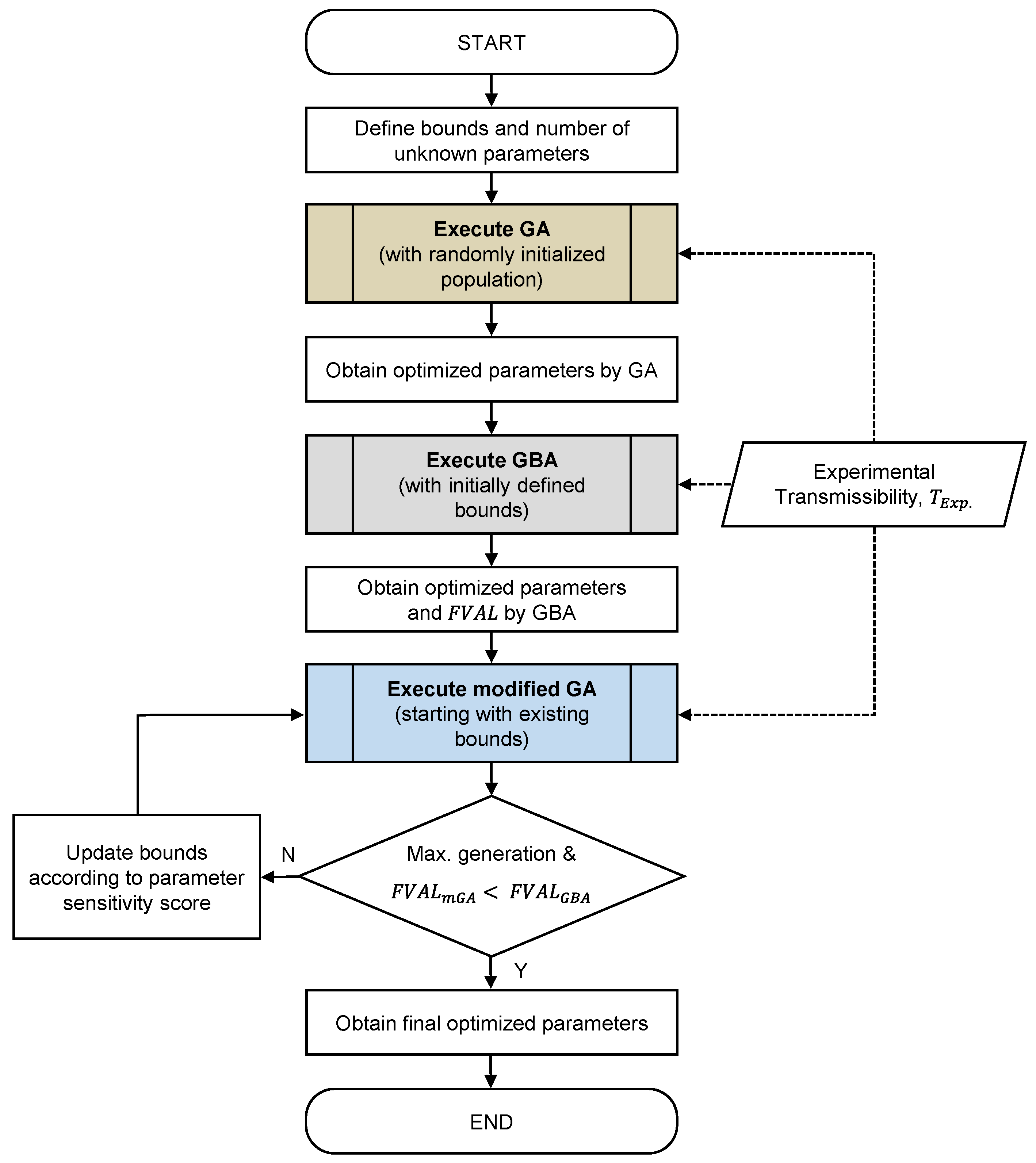
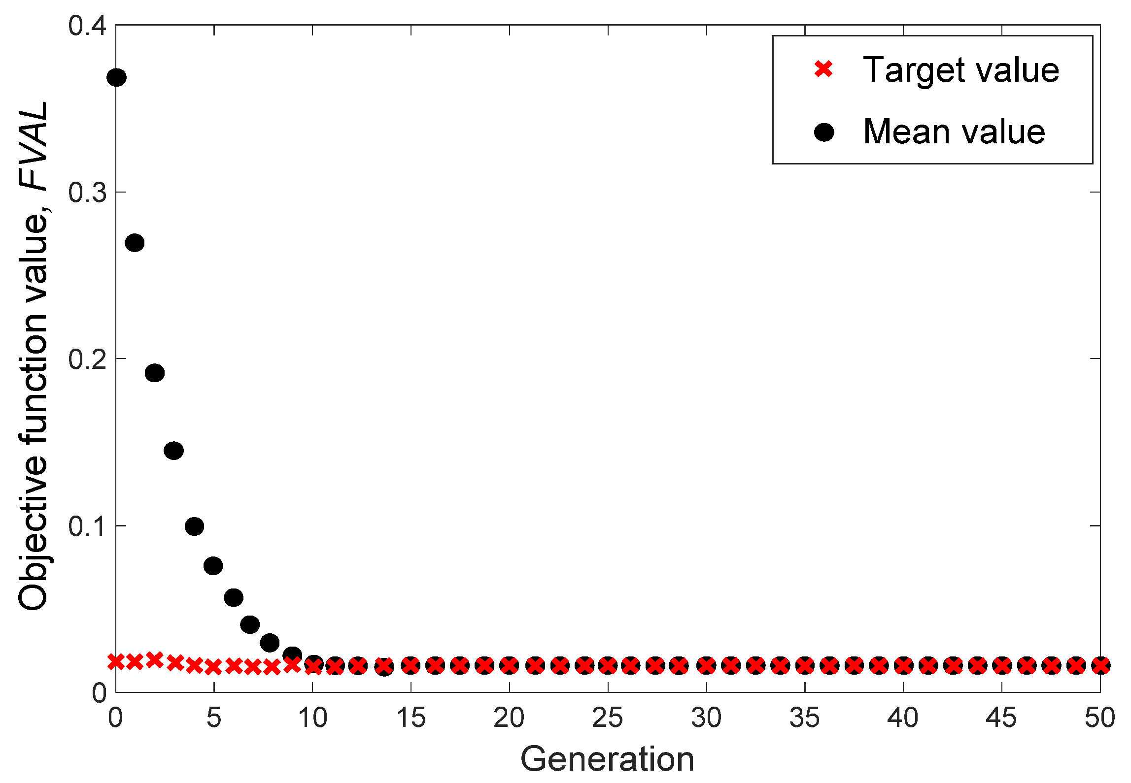
4.4. Hybrid Optimization Method (HOM)

The hybrid optimization method is developed to overcome the limitations of GBA and GA in the parameter estimation process (Figure 6). By combining the strengths of both algorithms, the HOM aims to improve the model fitting and reduce the randomness and exhaustive search for initial values involved in the optimization process. The first major step of HOM eliminates the exhaustive search encountered in GBA by using a typical random initial population-based GA. The computation parameters include an initial population size of 180, 18 elites, a crossover probability of 0.85, and the predefined parameters in the previous GA process. A mean FVAL of 0.0381 was returned after 1100 s in the GA process. In the second major step, GBA is used to explore the local optima of the near-global optimal solutions obtained by GA in the first step. We set the maximum iteration to 50, the maximum function evaluation to 2700, the step tolerance to 1 × 10^−15, and the function tolerance to 1 × 10⁻¹², with the optimized parameters from the first GA step as initial values.

For GBA. Interestingly, this step yielded a reduced FVAL of 0.0293 and a better fit of the transmissibility plots in the GBA process. Furthermore, we noticed that the values of some parameters obtained at different body segments varied only slightly while some remained unchanged.

In the third major step, we executed a modified GA (denoted as mGA) to address the randomness in optimized values exhibited by the typical GA, such as the one used in the first step. We defined an initial population matrix in the mGA and assigned values of the optimized parameters obtained by GBA as the elements of the population matrix. During this step, if FVAL by mGA is less than that by GBA in the previous step, a parameter sensitivity score is applied to update the bounds, and the mGA process is reinitiated. The final optimized parameters obtained in the mGA step are adapted as the HOM parameters. The HOM’s advantages over GBA and GA include improved model fitting, reduced randomness, and lower values of the objective function, making it a promising optimization method for parameter estimation in various applications.

5. Results

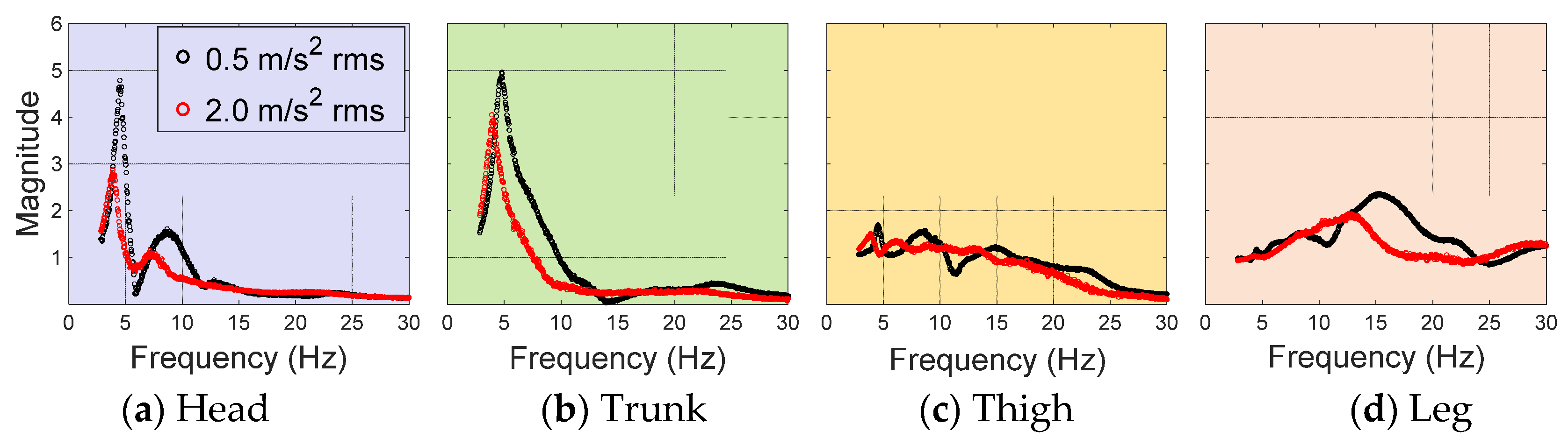
5.1. Experimental Results

Figure 7 shows the transmissibility obtained from processing the measured acceleration data described in the experimental section. The data is presented for four body segments: head, trunk, thigh, and leg. The results showed that the upper trunk and head segments have the highest magnitude of transmitted vibrations, both at 0.5 and 2.0 m/s² rms. The thigh and calf on the other hand are less susceptible to the transmitted vibrations.

Furthermore, at a forcing amplitude of 0.5 m/s² rms, all body segments exhibit a first principal resonant frequency in the range of 4–6 Hz, while the second principal reso-nance frequency is prominent in the head, thigh, and calf regions, within the range of 8–15 Hz. Our experimental approach confirms that the that the peak resonance fre-quencies of human response to vibration in the vertical direction are in the low-frequency region and the resonant frequencies obtained for each of the head, trunk, thigh and calf are in the region reported in literature [29,30,31].

Additionally, a non-linear response of the human body to an increase in excitation magnitude was observed for all the body segments. The ‘softening effect’ was observed as the excitation magnitude increased from 0.5 to 2.0 m/s² rms, indicating the strong non-linearity of human body biodynamics. Also, the peak magnitude of transmissibility at each body segment reduced, and the resonance frequency became less observable and diminished in magnitude as the vibration exposure time increased.

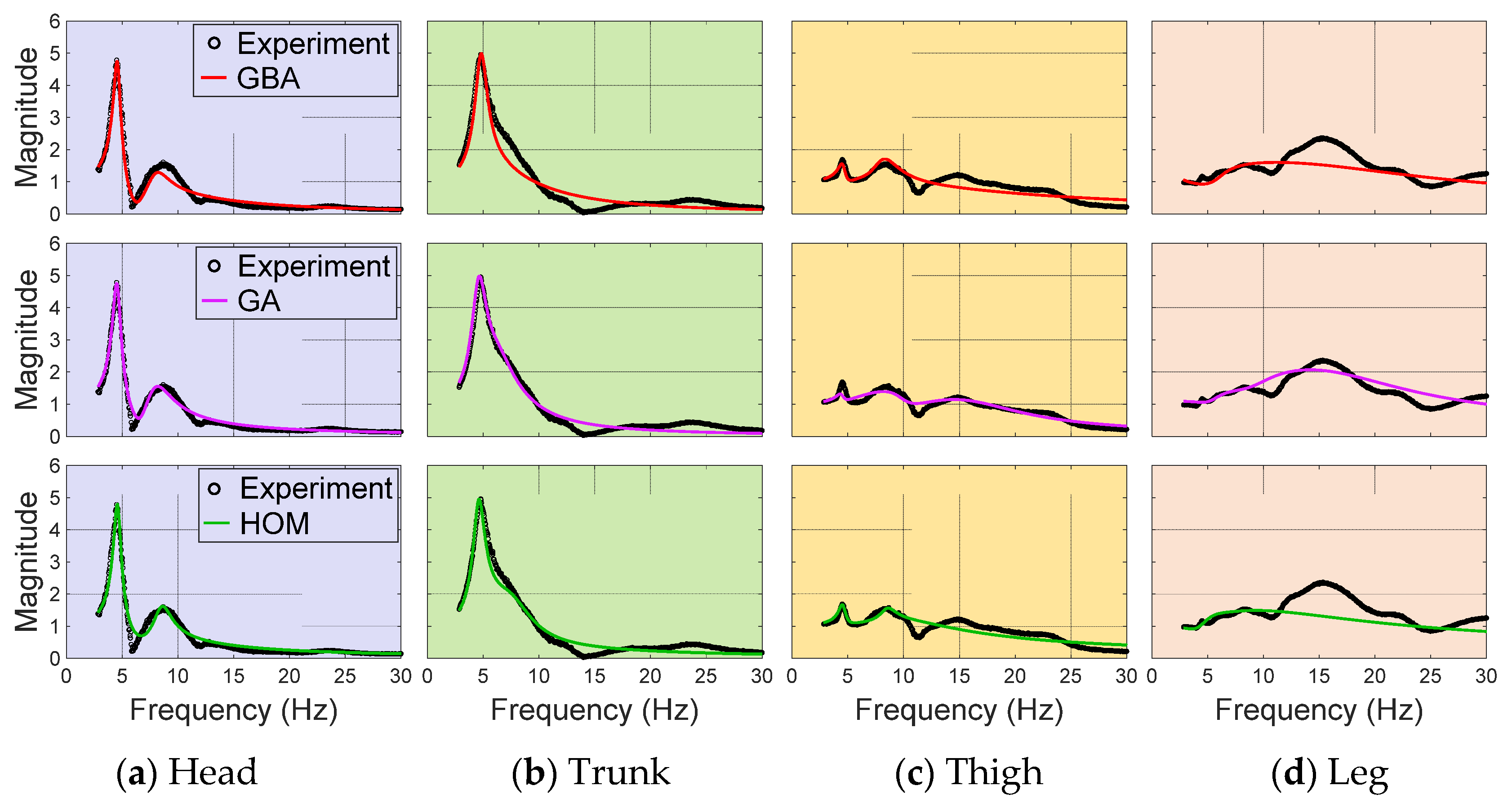
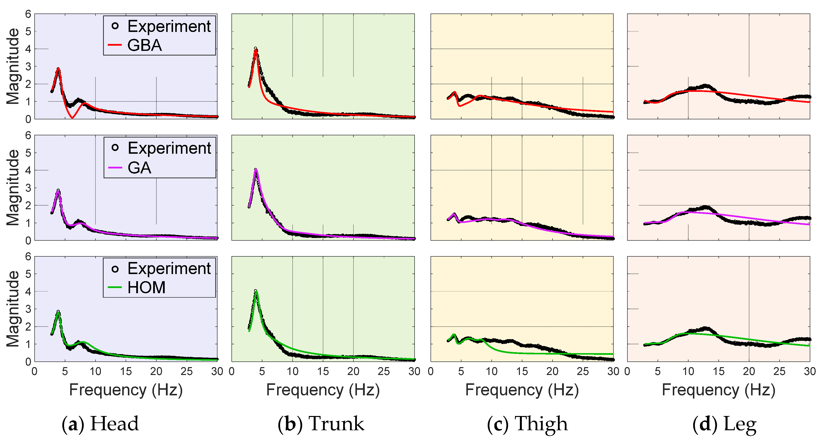
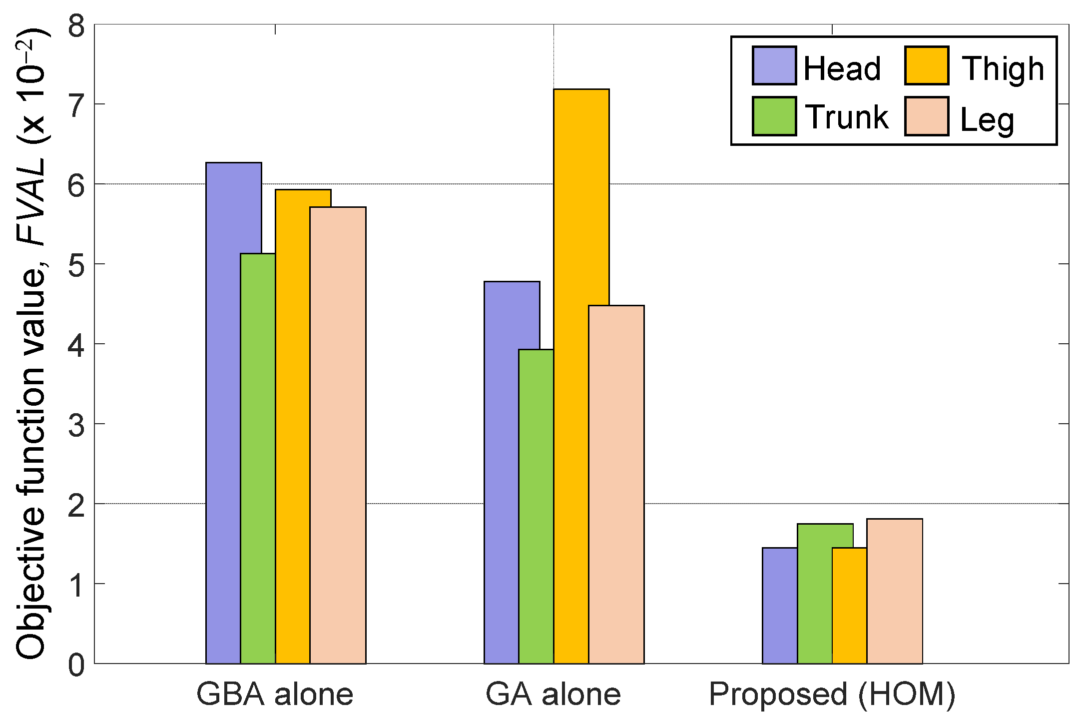
5.2. Model Fitting Results Obtained by the Optimization Methods

We analyzed the performance of the optimization methods in fitting the model by comparing results obtained by GBA, GA, and HOM. The model exhibited a strong fit to experimental data for all the optimization methods, with HOM showing the overall best fit at both 0.5 and 2.0 m/s² rms (Figure 8 and Figure 9). Furthermore, we established goodness of fit criteria, $\epsilon$ as suggested by Wong [32], to quantitatively evaluate the model-fitting results:

$$\epsilon =1-\left(\sqrt{\sum \frac{{\left(T_{Exp.}-T_{Model}\right)}^2}{N-2}}/\sum \frac{T_{Exp.}}{N}\right),$$

(26)

where N is the number of experimental data points used in the goodness of fit comparison. A value of $\epsilon$ close to 1 indicates a good fit, with values over 80% considered an acceptable tolerance of error for analysis. As shown in

Table 3. Goodness of fit at 0.5 m/s² rms.

Method	Head (%)	Trunk (%)	Thigh (%)	Leg (%)	Average (%)
GBA	95.8	92.5	94.6	82.8	91.4
GA	98.4	97.3	90.9	83.9	92.6
HOM	99.0	98.9	97.9	91.4	96.8

and

Table 4. Goodness of fit at 2.0 m/s² rms.

Method	Head (%)	Trunk (%)	Thigh (%)	Leg (%)	Average (%)
GBA	90.5	91.4	90.7	92.9	91.4
GA	99.9	99.5	93.4	94.2	96.7
HOM	99.5	98.9	98.7	95.9	98.2

, an average of 94% and 95% was obtained at forcing amplitude of 0.5 and 2.0 m/s² rms for all the optimization methods. The HOM achieved the highest ε value, signifying the best fit among the three optimization methods.

The performance of the optimization methods was also evaluated based on the objective function value at the final solutions, FVAL. Figure 10 demonstrates that when comparing the individual use of GBA or GA to the proposed method, HOM consistently achieved the lowest objective function value for all body segments. Moreover, by incorporating the GBA-optimized values in the MGA step, the computation process was expedited. The initial objective function value of approximately 0.400 rapidly decreased to a minimum of 0.0145 within the first 10 generations, as shown in Figure 11. Typically, the objective function values improve rapidly in initial generations and then level off as the optimal value is approached [28]. Detailed FVAL results for GBA, GA, and HOM for each body segment are presented in

Table 5. FVAL obtained when GBA and GA were used as standalone algorithms.

Method	Objective Function Value, FVAL
	Head	Trunk	Thigh	Leg
GBA alone	0.0478	0.0393	0.0719	0.0448
GA alone	0.0627	0.0513	0.0593	0.0571

and

Table 6. FVAL obtained for the combined HOM steps.

HOM Steps	Objective Function Value, FVAL
	Head	Trunk	Thigh	Leg
GA step	0.0328	0.0333	0.0394	0.0348
GBA step	0.0227	0.0293	0.0263	0.0301
MGA step	0.0145	0.0175	0.0145	0.0181

.

Furthermore, the computation time of HOM is significantly reduced compared to using GBA and GA separately. Specifically, the computation time of GBA and GA steps in the HOM process is over five times reduced for GBA and about 30% for GA, as shown in

Table 7. Computation time for each body segment when using GBA and GA alone.

Method	Computation Time (S)
	Head	Trunk	Thigh	Leg
GBA alone	1510	1620	1610	1760
GA alone	1310	1290	1310	1390

and

Table 8. Computation time for each body segment for combined HOM steps.

HOM Steps	Computation Time (S)
	Head	Trunk	Thigh	Leg
GA step	1066	1092	1066	1100
GBA step	210	200	206	260
MGA step	250	240	210	290
Total	1526	1532	1482	1650

. However, the combined time of HOM is still nearly the same as that of GA and a bit more than GBA.

Overall, the optimization methods performed well in fitting the model, with HOM being the most effective. The use of HOM also produced lower objective function values and faster computation time, which significantly improved the optimization process.

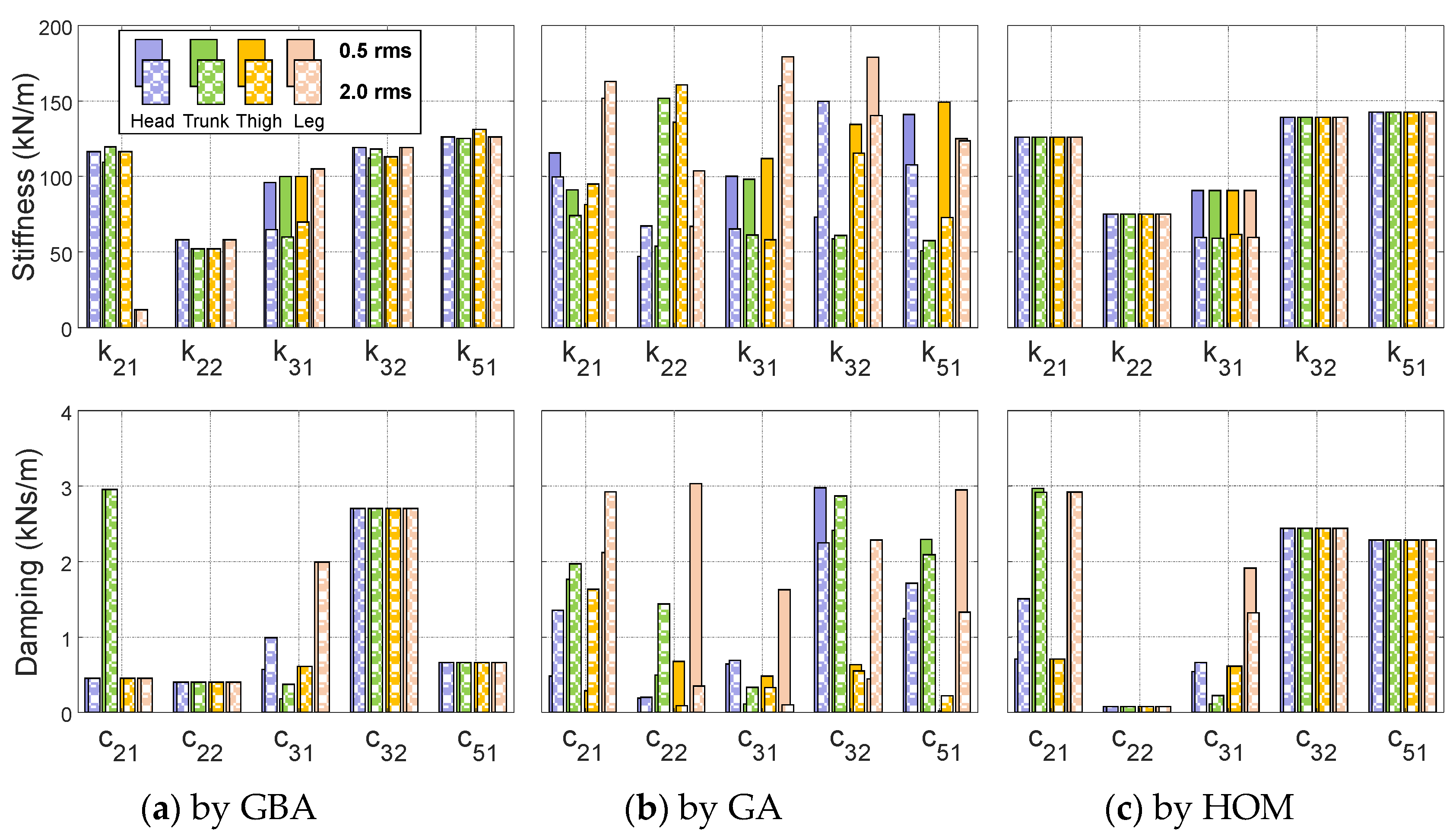
5.3. Estimated Parameters and Parameter Sensitivity

The stiffness and damping coefficients estimated by GBA, GA, and HOM for 10 translational parameters: $k_{21}$, $k_{22}$, $k_{31}$, $k_{32}$ and $k_{51}$ and $c_{21}$, $c_{22}$, $c_{31}$, $c_{32}$ and $c_{51}$ and 8 torsional parameters: $k_1^T$, $k_2^T$, $k_3^T$, $k_4^T$ and $c_1^T$, $c_2^T$, $c_3^T$, $c_4^T$ at 0.5 and 2.0 m/s² rms forcing magnitudes are presented in Figure 12 and Figure 13. The estimates were obtained by minimizing the squared error between the calculated and measured transmissibility for the head, trunk, thigh, and leg segments of the 7-DOF model. We analyzed the estimated parameters and compared the performance of each optimization method to gain insights into the key parameters that affect the appearance and magnitude of resonance frequencies and other modal characteristics of the model.

While HOM produced nearly the same values for the estimated translational and torsional parameters at either 0.5 or 2.0 m/s² rms for all body segments, GBA and GA showed significant variances for all estimated parameters. We attribute the high randomness in estimated parameters by GA to the nature of its random initial population assignment and that of GBA to the limitations of guessing the appropriate initial values for the estimated parameters.

To improve the results of estimated parameters, we performed a parameter sensitivity analysis by establishing a parameter sensitivity matrix, P with elements [26]:

$${\mathrm{P}}_{ij}=\frac{∆R_i/R_i}{∆{\psi }_j/{\psi }_j},$$

(27)

where $\psi =\left\{k_{21},k_{22},k_{31},k_{32},k_{51},c_{21},c_{22},c_{31},c_{32},c_{51},k_1^T,k_2^T,k_3^T,k_4^T,c_1^T,c_2^T,c_3^T,c_4^T\right\};$ ${\psi }_j$ and $∆{\psi }_j$ represent the $j$th ($j=\mathrm{1,2},\dots ,18$) parameter at its nominal value and its value after a small perturbation; $R_i$ represent the responses to be examined, in our case, the first resonance frequency ($i=1$), the second resonance frequency ($i=2$), the peak magnitude of resonance frequency ($i=3$), computed with the nominal value of each term in $\psi$, extracted from the final optimization results that allow us to fit the model to experiment as presented in Figure 8 and Figure 9; $∆R_i$ represent the differences in the value of the above responses after perturbation. We set the perturbation factor, $\alpha$ to 30% such that $∆{\psi }_j=\alpha {\psi }_j$ and the new values of each term in ${\psi }_j$, is ${\psi }_j^{new}={\psi }_j\pm ∆{\psi }_j$ with other parameters kept at their nominal values. Then, new values of each examined response, $R_i^{new}$ are computed with ${\psi }_j^{new}$ such that $∆R_i=\left|R_i^{new}-R_i\right|$.

At ±30%, the resultant parameter sensitivity matrix, normalized based on the maximum value in each row, is as follows:

$${\mathbf{P}}_{+30\mathrm{\%}}={\left[\begin{array}{ccc}0.02& 0.05& 0.00\\ 0.00& 0.00& 0.00\\ \mathbf{1.00}& \mathbf{1.00}& 0.09\\ 0.01& 0.01& 0.00\\ \mathbf{0.41}& \mathbf{0.31}& 0.02\\ \mathbf{0.21}& 0.05& \mathbf{0.91}\\ 0.01& 0.00& 0.00\\ 0.02& 0.01& \mathbf{1.00}\\ 0.00& 0.00& 0.03\\ 0.09& 0.00& \mathbf{0.32}\\ 0.00& 0.00& 0.00\\ 0.00& 0.00& 0.00\\ 0.00& 0.00& 0.00\\ 0.00& 0.00& 0.00\\ 0.02& 0.01& 0.05\\ 0.05& 0.01& 0.04\\ 0.00& 0.00& \mathbf{0.86}\\ 0.06& 0.03& 0.01\end{array}\right]}^T \mathrm{and} {\mathbf{P}}_{-30\%}={\left[\begin{array}{ccc}0.05& 0.08& 0.00\\ 0.00& 0.00& 0.00\\ \mathbf{1.00}& \mathbf{1.00}& 0.05\\ 0.01& 0.00& 0.00\\ \mathbf{0.52}& \mathbf{0.49}& 0.01\\ \mathbf{0.28}& 0.06& \mathbf{0.85}\\ 0.02& 0.00& 0.00\\ 0.02& 0.01& \mathbf{1.00}\\ 0.00& 0.00& 0.04\\ 0.05& 0.00& \mathbf{0.38}\\ 0.00& 0.00& 0.00\\ 0.00& 0.00& 0.00\\ 0.00& 0.00& 0.00\\ 0.00& 0.00& 0.00\\ 0.01& 0.01& 0.03\\ 0.02& 0.01& 0.02\\ 0.00& 0.00& \mathbf{0.78}\\ 0.08& 0.05& 0.01\end{array}\right]}^T$$

For each examined response, the sensitivity of each parameter was analyzed based on their score in the parameter sensitivity matrix. The greater the value, the more sensitive the parameter is to the considered response. The values from the matrix show that $k_{31}$, $k_{51}$, $c_{21}$, $c_{31}$, $c_{51}$ and $c_3^T$ are the most significant parameters to the appearance and magnitude of the resonance frequency.

Table 9. Summary of sensitivity of key parameters to the appearance and magnitude of the resonance frequency at ±30% perturbation.

Examined Responses	Decreasing Order of Sensitivity
First resonance frequency	$k_{31}, k_{51}, c_{21}$
Second resonance frequency	$k_{31}, k_{51}$
Peak magnitude of resonance frequency	$c_{31}, c_{21}, c_3^T, c_{51}$

summarizes the order of sensitivity of these parameters for the examined responses.

We utilized the sensitivity matrix score to update the bounds in the mGA repeatedly and extracted the final optimized parameters. This process allowed us to obtain numerically stable values for each of $k_{21}$, $k_{22}$, $k_{31}$, $k_{32}$ and $k_{51},$ whose estimated values remained unchanged at 0.5 m/s² rms regardless of the body segment transmissibility data used in the objective function (Figure 12). Similarly, at 2.0 m/s² rms, all the $k_{ij}$ terms remained consistent except $k_{31}$, whose value reduced slightly for all body segments, confirming the ‘softening effect’ observed in the experimental results. The reduction in $k_{31}$ as the excitation magnitude increased, suggested the softening in the stiffness of the tissue beneath the ischial tuberosities, as reported in the literature [27,33]. As observed with the $k_{ij}$ terms, values of $c_{22}$, $c_{32}$ and $c_{51}$ were consistent, while the variances in values of $c_{21}$ and $c_{31}$ for some of the body segments can be associated with their sensitivity to the magnitude of resonance frequency.

Also, as presented in Figure 13, the torsional parameters for HOM showed nearly the same values across all body segments and forcing magnitudes. Particularly, the torsional stiffness coefficients, $k_{\mathrm{i}}^T$ were unchanged. The changes in the torsional damping, especially $c_3^T$ is associated with its high significance in determining the magnitude of the resonance frequencies.

6. Discussions

6.1. Proposed Model

The proposed 7-DOF seated human model was successfully validated for its intended application in predicting the response of distinct body segments to vertical vibration in the low-frequency range of 0–15 Hz. We were able to access the response of each body segment with increasing excitation magnitude, with the upper trunk and head showing the most susceptibility to transmitted vibration. Also, the model accurately captured the resonant frequencies of each body segment observed in the experimental results. Furthermore, the model demonstrated the ability to exhibit non-linearity in human biodynamics despite its simplicity by replicating the “softening effect.”

The high goodness-of-fit scores obtained during the model fitting process suggest that the proposed model is effective with different optimization algorithms. The validated model can be used in future research to optimize the comfort and safety of individuals in various seating arrangements. However, it is important to acknowledge the limitations of the proposed model, including its applicability in the high-frequency range and the limited number of experimental subjects. Further studies are necessary to address these limitations and enhance the model’s applicability in diverse scenarios.

6.2. Estimation of Unknown Parameters Using Proposed HOM

The lack of established data on human parameters, such as stiffness and damping coefficients, highlights the significance of developing an effective parameter optimization algorithm. In this study, the proposed HOM was able to combine the strengths of typical GBA and GA to estimate the unknown stiffness and damping coefficients. Not only did HOM outperform GBA and GA in terms of goodness of fit, but it also achieved the lowest objective function values at faster computation speeds.

Furthermore, the combination of the 7-DOF model and HOM revealed that the unknown human parameters, particularly stiffness, could be estimated using data measured from any of the body segments, with minor variations in optimized values across different excitation magnitudes. Also, Figure 12 demonstrates that the spring-damper at the foot, distal fragment of the thigh, and the lower trunk are stiffer than those at the upper trunk and proximal fragment of the thigh. This suggests that the vibration transmitted through the seat is greater than that through the foot. Also, the upper trunk, being less stiff, experiences more displacement, leading to more displacement of the head segment and the potential for motion sickness, as suggested by Bovenzi [2]. Similarly, the high displacement (lower stiffness) exhibited by the spring damper at the buttock region can account for the reduction in k₃₁ at increased excitation magnitude, implying the softening of the tissue beneath the ischial tuberosities.

7. Conclusions

In this study, we successfully developed a seven-degree-of-freedom (7-DOF) model under vertical vibration and estimated 18 effective stiffness and damping coefficients using a new hybrid optimization method. The goal was to understand how vibration is transmitted to distinct human body segments, especially in the low-frequency region, by analyzing the estimated parameters by GBA, GA, and HOM using transmissibility responses from experiments and those calculated using the 7-DOF model. Results from experiments showed that the upper trunk and head are most susceptible to transmitted vibrations, with the thigh and leg showing lesser magnitudes. Also, the peak magnitude of transmissibility at each body segment reduced, and the resonance frequency became less observable and diminished in magnitude as the vibration exposure time increased.

Our findings also showed that combining the 7-DOF model with the hybrid optimization method significantly accelerated the optimization process, enhanced numerical stability, and resulted in a significant reduction of the objective function value compared to using GBA or GA as standalone algorithms. Additionally, HOM was more suitable for the estimation of the unknown stiffness and damping parameters. Notably, we found that unknown human parameters, particularly stiffness, could be estimated using data measured from any of the body segments, with minor variations in optimized values across different excitation magnitudes. Finally, the ‘softening effect’ was observed as the excitation magnitude increased from 0.5 to 2.0 m/s² rms., indicating the strong non-linearity of human body biodynamics.

These results have practical implications for optimizing the comfort and safety of individuals exposed to whole-body vibration when riding in vehicles, as ergonomists and design engineers can use the developed model and HOM to identify the body segments most susceptible to vibration. Future work will focus on studying the correlation of transmissibility at different points on each body segment, the effects of subject variabilities, and the addition of lateral excitation.

References

1. Bovenzi, M.; Betta, A. Low-back disorders in agricultural tractor drivers exposed to whole-body vibration and postural stress. Appl. Ergon. 1994, 25, 231–241. [Google Scholar] [CrossRef] [PubMed]
2. Bovenzi, M.; Hulshof, C.T.J. An Updated Review of Epidemiologic Studies on the Relationship Between Exposure to Whole-Body Vibration and Low Back Pain (1986–1997). Int. Arch. Occup. Environ. Health 1999, 72, 351–365. [Google Scholar] [CrossRef] [PubMed]
3. International Organization for Standardization (ISO). Mechanical Vibration and Shock: Range of Idealized Values to Characterize Seated-Body Biodynamic Response under Vertical Vibration; International Organization for Standardization: Geneva, Switzerland, 2002. [Google Scholar]
4. Zhou, Z.; Griffin, M.J. Response of the Seated Human Body to Whole-Body Vertical Vibration: Discomfort Caused by Sinusoidal Vibration. Ergonomics 2014, 57, 714–732. [Google Scholar] [CrossRef]
5. Kim, E.; Fard, M.; Kato, K. Characterisation of the Human-seat Coupling in Response to Vibration. Ergonomics 2017, 60, 1085–1100. [Google Scholar] [CrossRef] [PubMed]
6. Rakheja, S.; Dewangan, K.N.; Dong, R.G.; Marcotte, P.; Pranesh, A. Whole-Body Vibration Biodynamics—A Critical Review: II. Biodynamic Modelling. Int. J. Veh. Perform. 2020, 6, 52–84. [Google Scholar] [CrossRef]
7. Matsumoto, Y.; Griffin, M.J. Non-linear Characteristics in the Dynamic Responses of Seated Subjects Exposed to Vertical Whole-Body Vibration. J. Biomech. Eng. 2002, 124, 527–532. [Google Scholar] [CrossRef]
8. Cho, Y.; Yoon, Y.S. Biomechanical Model of Human on Seat With Backrest for Evaluating Ride Quality. Int. J. Ind. Ergon. 2001, 27, 331–345. [Google Scholar] [CrossRef]
9. Kim, T.H.; Kim, Y.T.; Yoon, Y.S. Development of a biomechanical model of the human body in a sitting posture with vibration transmissibility in the vertical direction. Int. J. Ind. Ergon. 2005, 35, 817–829. [Google Scholar] [CrossRef]
10. Bae, J.J.; Kang, N. Development of a Five-Degree-of-Freedom Seated Human Model and Parametric Studies for its Vibrational Characteristics. Shock Vib. 2018, 2018, 1649180. [Google Scholar] [CrossRef]
11. Tufano, S.; Griffin, M.J. Nonlinearity in the vertical transmissibility of seating: The role of the human body apparent mass and seat dynamic stiffness. Veh. Syst. Dyn. 2013, 51, 122–138. [Google Scholar] [CrossRef]
12. Dewangan, K.N.; Rakheja, S.; Marcotte, P.; Shahmir, A. Effects of elastic seats on seated body apparent mass responses to vertical whole-body vibration. Ergonomics 2015, 58, 1175–1190. [Google Scholar] [CrossRef] [PubMed]
13. Wang, W.; Rakheja, S.; Boileau, P.É. Effect of back support condition on seat to head transmissibilities of seated occupants under vertical vibration. J. Low Freq. Noise Vib. Act. Control 2006, 25, 239–259. [Google Scholar] [CrossRef]
14. Matsumoto, Y.; Griffin, M.J. Modelling the dynamic mechanisms associated with the principal resonance of the seated human body. Clin. Biomech. 2001, 16, S31–S44. [Google Scholar] [CrossRef] [PubMed]
15. Shao, X.; Xu, N.; Liu, X. Investigation and Application on the Vertical Vibration Models of the Seated Human Body. Automot. Innov. 2018, 1, 263–271. [Google Scholar] [CrossRef]
16. Huang, Y.; Zhang, P.; Liang, S. Apparent mass of the seated human body during vertical vibration in the frequency range 2–100 Hz. Ergonomics 2020, 63, 1150–1163. [Google Scholar] [CrossRef]
17. Zhang, S.; Shi, W.; Chen, Z. Modeling and Parameter Identification of Seated Human Body with the Reference Vector Guided Evolutionary Algorithm. Adv. Mech. Eng. 2021, 13, 16878140211062679. [Google Scholar] [CrossRef]
18. Zhao, Y.; Alashmori, M.; Bi, F.; Wang, X. Parameter Identification and Robust Vibration Control of a Truck Driver’s Seat System Using Multi-Objective Optimization and Genetic Algorithm. Appl. Acoust. 2021, 173, 107697. [Google Scholar] [CrossRef]
19. Yazdi, S.J.M.; Cho, K.S.; Kang, N. Characterization of the Viscoelastic Model of In Vivo Human Posterior Thigh Skin using Ramp-Relaxation Indentation Test. Korea-Aust. Rheol. J. 2018, 30, 293–307. [Google Scholar] [CrossRef]
20. Zhang, X.; Yu, P.; Li, Y.; Qiu, Y.; Sun, C.; Wang, Z.; Liu, C. Dynamic Interaction Between the Human Body and the Seat During Vertical Vibration: Effect of Inclination of the Seat Pan and the Backrest on Seat Transmissibilities. Ergonomics 2022, 65, 691–703. [Google Scholar] [CrossRef]
21. Xiu, W.; Zhang, L.; Ma, O. Experimental study of a momentum-based method for identifying the inertia barycentric parameters of a human body. Multibody Syst. Dyn. 2016, 36, 237–255. [Google Scholar] [CrossRef]
22. Size Korea. The 8th Korean Human Dimensions Survey Project. Available online: https://sizekorea.kr/human-info/meas-report?measDegree=8 (accessed on 15 March 2021).
23. Ma, Y.; Kwon, J.; Mao, Z.; Lee, K.; Li, L.; Chung, H. Segment Inertial Parameters of Korean Adults Estimated from Three-Dimensional Body Laser Scan Data. Int. J. Ind. Ergon. 2011, 41, 19–29. [Google Scholar] [CrossRef]
24. Kim, K.S.; Kim, J.; Kim, K.J. Dynamic Modeling of Seated Human Body Based on Measurements of Apparent Inertia Matrix for Fore-and-Aft/Vertical/Pitch Motion. J. Sound Vib. 2011, 330, 5716–5735. [Google Scholar] [CrossRef]
25. Liang, C.C.; Chiang, C.F. Modeling of a Seated Human Body Exposed to Vertical Vibrations in Various Automotive Postures. Ind. Health 2008, 46, 125–137. [Google Scholar] [CrossRef] [PubMed]
26. Qiu, Y.; Griffin, M.J. Modelling the fore-and-aft apparent mass of the human body and the transmissibility of seat backrests. Veh. Syst. Dyn. 2011, 49, 703–722. [Google Scholar] [CrossRef]
27. Wu, J.; Qiu, Y.; Sun, C. Modelling and analysis of coupled vibration of human body in the sagittal and coronal planes exposed to vertical, lateral and roll vibrations and the comparison with modal test. Mech. Syst. Signal Proc. 2022, 166, 108439. [Google Scholar] [CrossRef]
28. Math Works, Inc. Genetic Algorithm and Direct Search Toolbox for Use with MATLAB: User’s Guide. Available online: http://cda.psych.uiuc.edu/matlab_pdf/gads_tb.pdf (accessed on 2 May 2023).
29. Fairley, T.E.; Griffin, M.J. The apparent mass of the seated human body: Vertical vibration. J. Biomech. 1989, 22, 81–94. [Google Scholar] [CrossRef]
30. Nawayseh, N.; Griffin, M.J. Non-linear dual-axis biodynamic response to vertical whole-body vibration. J. Sound Vibr. 2003, 268, 503–523. [Google Scholar] [CrossRef]
31. Wu, J.; Qiu, Y. Modelling of Seated Human Body Exposed to Combined Vertical, Lateral and Roll Vibrations. J. Sound Vibr. 2020, 485, 115509. [Google Scholar] [CrossRef]
32. Wong, J.Y. Terramechanics and Off-Road Vehicle Engineering: Terrain Behaviour, Off-Road Vehicle Performance and Design; Butterworth-Heinemann: Oxford, UK, 2009. [Google Scholar]
33. Mansfield, N.J.; Griffin, M.J. Non-linearities in apparent mass and transmissibility during exposure to whole-body vertical vibration. J. Biomech. 2000, 33, 933–941. [Google Scholar] [CrossRef]
Figure 1. The proposed 7-DOF seated human model.
Applsci 13 10065 g001
Figure 2. The deformed and undeformed configurations of the 7-DOF model during vibrations.
Applsci 13 10065 g002
Figure 3. Detailed schematic of deflection of the spring damper.
Applsci 13 10065 g003
Figure 4. Equipment used for vibration excitation and the mounted vehicle seat.
Applsci 13 10065 g004
Figure 5. The NexGen monitoring system and locations of IMU sensors on the subject.
Applsci 13 10065 g005
Figure 6. Hybrid optimization method (HOM) flowchart.
Applsci 13 10065 g006
Figure 7. Transmissibility obtained from experiments at 0.5 and 2.0 m/s2 rms forcing magnitudes.
Applsci 13 10065 g007
Figure 8. Model fitting results obtained by GBA, GA, and HOM at 0.5 m/s2 rms forcing amplitude.
Applsci 13 10065 g008
Figure 9. Model fitting results obtained by GBA, GA, and HOM at 2.0 m/s2 rms forcing amplitude.
Applsci 13 10065 g009
Figure 10. Comparison of the objective function values by optimization methods.
Applsci 13 10065 g010
Figure 11. Target and mean value of FVAL by mGA with respect to the generations of evolution in the HOM process.
Applsci 13 10065 g011
Figure 12. Translational parameters (top: stiffness coefficients, bottom: damping coefficients).
Applsci 13 10065 g012
Figure 13. Torsional parameters (top: stiffness coefficients, bottom: damping coefficients).
Applsci 13 10065 g013