1. Introduction
To successfully connect incoming calls to the correct user equipment (UE), wireless communication networks use methods that track the current location of the UE. Many wireless resources are utilized for these mobility management methods [
1,
2,
3,
4,
5]. Mobility management consists of two operations: location registration and paging [
1,
6,
7]. Location registration is a process wherein the network database modifies the current location of the UE each time the UE moves to a new registration area (RA) to report its current location to the network. In that system, the RA is composed of several zones, where each zone is comprised of several cells that do not overlap with each other [
8,
9]. Paging is the process of sending a paging message to all zones that are included in the RA to which the UE belongs whenever an incoming call arrives. Therefore, depending on the size of the RA (that is, the number of zones inside an RA), the numbers of registrations and paging messages vary according to the UE’s movement, leading to substantial changes in the cost of wireless signaling traffic [
4,
10,
11,
12,
13].
To date, many schemes have been proposed to minimize signaling costs at radio frequencies, which can be classified into zone-based [
1,
8,
14,
15,
16,
17], distance-based [
18,
19], movement-based [
20,
21], timer-based [
1,
4,
22,
23], and so on [
9,
13,
24,
25]. Among these schemes, a zone-based registration scheme is employed by most wireless communication networks due to its good performance and convenient implementation [
1,
5]. Nevertheless, the biggest disadvantage of a zone-based method is the registration traffic generated by UEs that frequently enter and exit the RA boundary. To improve the performance when only one zone is included in RA (1Z), systems having two zones (2Z) or three zones (3Z) have been proposed [
15,
16,
17]. Those studies evaluated the performances of 2Z and 3Z while assuming a square-shaped zone. However, considering the actual situation, it is difficult to say that a square best represents the shape of the zone. Rather, many studies have used more hexagonal zones that extend widely adopted hexagonal cells [
3,
8,
10,
18,
21]. In this study, we analyzed the performances of 1Z, 2Z, and 3Z for a hexagonal-shaped zone by creating exact models of two types of 3Z structures in more realistic wireless network environments.
This study focused on the zone-based registration method and evaluated the performance of the 3Z system in the form of a hexagonal-shaped zone. To analyze the performance of the 3Z, the semi-Markov process theory [
26] was used to obtain the steady-state probability and compare its performance with those of 1Z and 2Z systems.
The rest of this paper proceeds as follows:
Section 2 defines all feasible states when three hexagonal zones are operated as one RA. This section also mathematically models the transition probability between states, the probability that registration will be required during a state transition, and the number of paging messages. In
Section 3, the steady-state probability is obtained from the state transition probability, after which the registration and paging cost incurred per UE are computed using steady-state probability. Subsequently,
Section 4 compares the performances of 1Z, 2Z, and 3Z systems under realistic parameter values. Finally, the conclusion is presented in
Section 5.
2. Zone-Based Registration Scheme
In this study, we assumed that the number of cells in each zone was
n and that the zone had a hexagonal shape. Moreover, the number of zones included in each RA was defined as a 1Z system when it had one zone, a 2Z system when it had two zones, and a 3Z system when it had three zones.
Figure 1 shows the location registration process due to UE’s movement for each system. UE moved from 3→2→1, changed direction, and then moved back to zone 1→2→3. First, in 1Z, a new registration was required whenever UE left the zone, resulting in four registrations in total. In 2Z, since the UE and network stored two zones in the database (DB), the registration procedure did not occur if it returned from zone 1 to zone 2. Accordingly, if the incoming call arrived when the UE remained in zone 2, then the UE would be connected with two paging processes. That is, in 2Z, since the registration process was not carried out when the UE moved from 1→2, the network database (Network_DB) knew that the UE was in zone 1. Thus, a call connection was made possible by paging zone 2 without receiving a response after paging zone 1 while the UE remained in zone 2.
Finally, in a 3Z system, no registration was required when moving among three zones belonging to the same RA. Similarly, if the UE stayed in zone 2, then two paging messages occurred, while when it was in zone 3, three paging procedures were needed. Note that in DB =
,
a was the most recently visited (or registered) zone,
b was the previously registered zone, and
c was the oldest visited zone. Unlike in previous studies [
16,
17], when a hexagonal zone was assumed, the 3Z scheme should be analyzed in consideration of two different types, as shown in
Figure 1. Type I was defined as having three zones registered sequentially without forming a cluster. By contrast, Type II was a case where three zones formed a cluster with the number of surfaces in contact being three.
To analyze the performance of 3Z, we assumed the following mobility models:
- (1)
The number of cells in each zone was assumed to be n. As analyzed in [
27,
28], it should be analyzed assuming UE’s movement between cells. However, when n was large (usually 7 or more), the shape of the zone became close to a hexagonal shape. Thus, a mobility model between zones was adopted. Note that in 1Z, registration would be required if the zone changed, not when the cell changed.
- (2)
Adopting a random-walk mobility model [
16,
17,
26], the UE moved to one of the six neighboring zones, where the probability of it returning to the previously visited zone was
θ. Thus, the probability of it moving to one of the other five adjacent zones was equal to (1 −
θ)/5.
- (3)
The number of calls to be processed per unit of time followed a Poisson distribution with a mean of
λ. Due to the additive nature of the Poisson process [
26], the
λ could be expressed as the sum of the number of outgoing calls (
λo) and incoming calls (
λi) treated during unit time (
λ =
λo +
λi).
- (4)
Based on the above assumption (2), the time interval, Tc, between two calls followed an exponential distribution with a mean of 1/λ.
- (5)
The time,
Tm, that the UE stayed in each zone followed a general distribution with an average of E(
Tm) = 1/
μ. When a call occurred to the UE, the UE’s location information in the network database could be modified using an implicit registration process [
1,
15] without any additional registration cost. The call-to-mobility ratio (CMR) was then defined as CMR =
λ/
μ. The case of CMR = 1 implied a situation in which the UE entered another zone once on average until the next call occurred.
- (6)
The probability,
m, that no call would occur until the UE entered a new zone was derived as follows:
where
was the Laplace–Stieltjes transform for
Tm ). Thus,
was the probability of a call occurring before leaving the zone, in which case the implicit registration was performed after the call was connected. Note that if a call occurred while UE stayed in the zone, the implicit registration was processed. If UE moved to another new zone before the call occurred, registration was required.
- (7)
The time remaining in the zone after a call occurrence was defined as a random variable
Rm. The
was a probability density function for
Rm, which could be easily obtained using the random observer property [
8,
26]:
Further, the Laplace–Stieltjes transform for
Rm was
- (8)
After the call processing, the UE would stay in the zone during
Rm. Using Equations (2) and (3), we could derive the probability,
m′, that another call would not happen again while the UE stayed in the zone:
Likewise, denoted the probability of another call connection before Rm, and Network_DB could be updated by implicit registration.
- (9)
Compared to times (
Tm and
Rm) of staying in the zone, the call duration was negligibly small [
4,
5,
9,
16,
17,
21]. Under this assumption, we could obtain
m and
m′ normally.
It is now necessary to define the states for the two types described in
Figure 1. To define the status of UE, three different cases for UE’s movements were considered for each of the two types as follows:
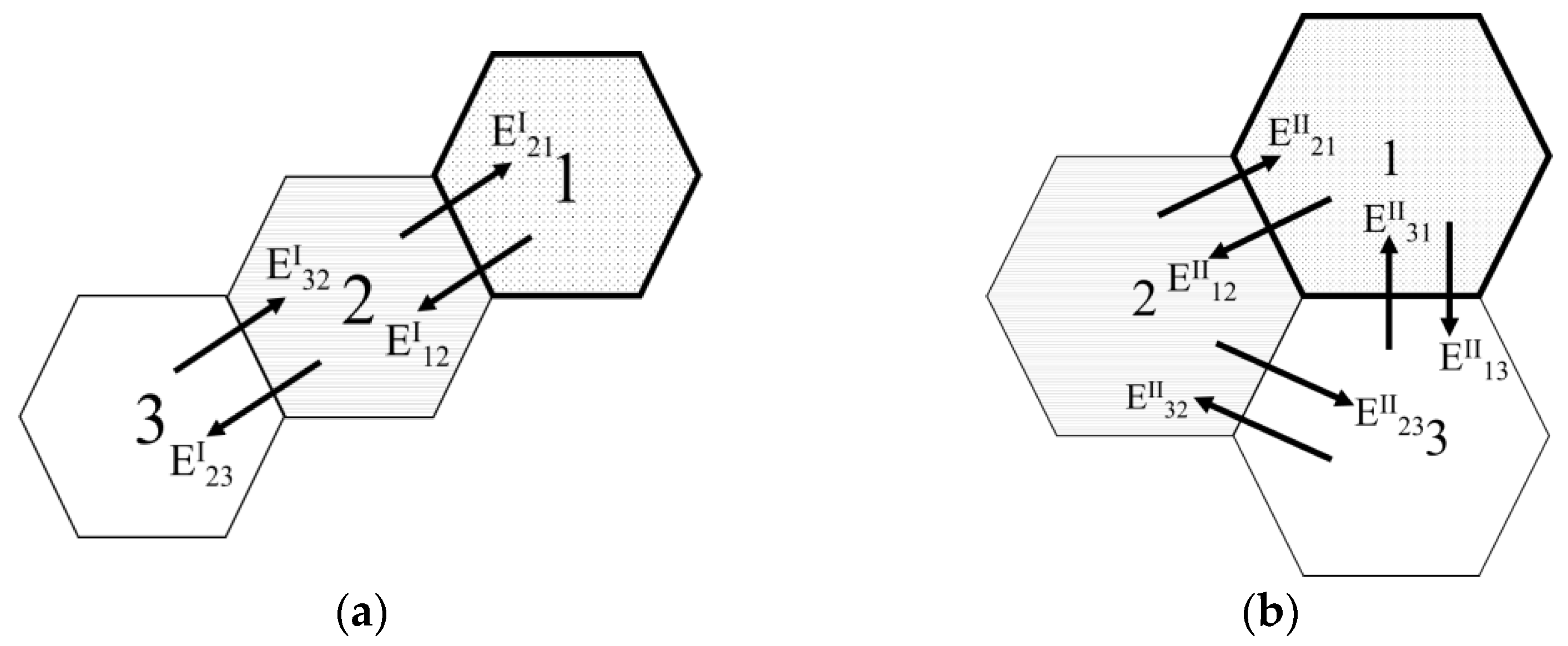
Case 1: Three different zones form one RA, and the UE travels inside these zones. In particular, in Type I, the most recently registered zone belongs to the boundary of RA. As depicted in
Figure 2, four states can be defined for Type I, whereas six states can be defined for Type II. Here, states
and
represent a case of moving from zone
i to zone
j for Types I and II, respectively. For example, state
indicates the state in which the UE remains in zone 3 after the UE moves to 3→2→1, stores three zones as RA, and then moves to 1→2→3 without an additional registration. In this state, if a call arrives to the UE, then three paging processes are required (1→2→3). That is, after paging zones 1 and 2, a response is not received. However, after zone 3 is paged, the call can be connected.
Case 2: This is a case in which an incoming (or outgoing) call is generated while UE stays in the RA. Hence, UE’s location information can be modified in the network database without requiring an additional registration procedure. This process is called implicit registration [
1,
15].
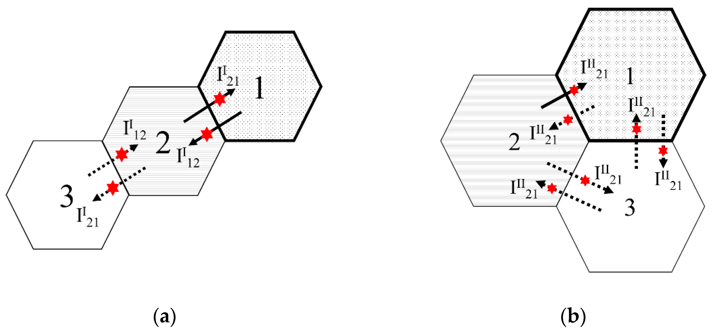
Figure 3 shows the states in which implicit registration occurs for each type. States
and
are defined as the states in which the call is processed while the UE resides in zone
j after arriving from zone
i for each type. Namely, the state
shows that the UE moves to 3→2→1, returns to zone 2, and then a call occurs in zone 2, thus allowing Network_DB to store UE’s location (
) without an additional registration cost. Note that for Type I, states
and
(or
and
) can be defined as the same states due to symmetric movements of the UE. We defined states
and
as situations in which a call occurred after the UE moved from middle zone 2 to edge zone 1 (or 3), after which Network_DB became
. On the other hand, states
and
represented the states in which the UE moved from edge zone 1 (or 3) to middle zone 2, and then a call was generated, and Network_DB became
.
Unlike Type I, Type II does not require a separate distinction between the center and edge because it is a clustered-shape RA. Thus, there is no need to define state
separately. That is, in Type 2, the one state definition of
is sufficient as shown in
Figure 3b. If the UE moves from zone 1 to zone 2 and implicit registration occurs in zone 2, then the Network_DB has
, and the Network_DB eventually has the most recently registered zone in the first entry, while the second entry has the zone previously visited. Afterward, considering the UE’s movement inside the hexagonal RA configuration, it can be seen that all transferable state transitions in each zone are the same after processing the implicit registration in RA. Note that in Case 2, if an incoming call is generated before moving from the zone processed by the implicit registration to another zone, the UE could be located through one paging message.
Case 3: This refers to a case where the UE generates a call in the second registered zone. In other words, when a call occurs in zone 2, as shown in
Figure 4, the location information of UE could be modified in the network without requiring another registration. State
in Type I implies a situation in which the UE moves from zone
i to
j without an additional registration while storing Network_DB =
after a call is generated in zone 2. In this case, it is necessary to have four different states for Type I to be defined. That is, unlike Case 2, it should be noted that states
and
must be defined differently. This is because in state
, the Network_DB is
. If an incoming call arrives in zone 1, then two paging processes (2→1) are needed. By contrast, for state
, since Network_DB has the same information of
, three paging processes are required while residing in zone 3. Further, for Type II, since the state transition to other states is always the same after call occurrence in each zone, there is no need for an additional state definition for Case 3. Note that we can utilize state
if the call is generated in one of the three zones for Type II.
According to the three cases presented above, 10 states are defined for Type I and 7 states are defined for Type II. Thus, 17 states in total are used to analyze the 3Z system. To find the steady-state probability for these states, it is necessary to determine the transition probabilities between states. In the following, a method of obtaining the transition probability between states will be described based on classifications for each type.
2.1. Type I: Serial Shape
In Type I, the state definitions for the three cases and the transition probability between states are explained as follows.
2.1.1. Case 1: Moving inside the Three Zones after Forming a Serial-Shaped RA
Four states can be defined, as shown in
Figure 2 when the UE travels without a separate registration process within the RA after configuring a serial-shaped RA.
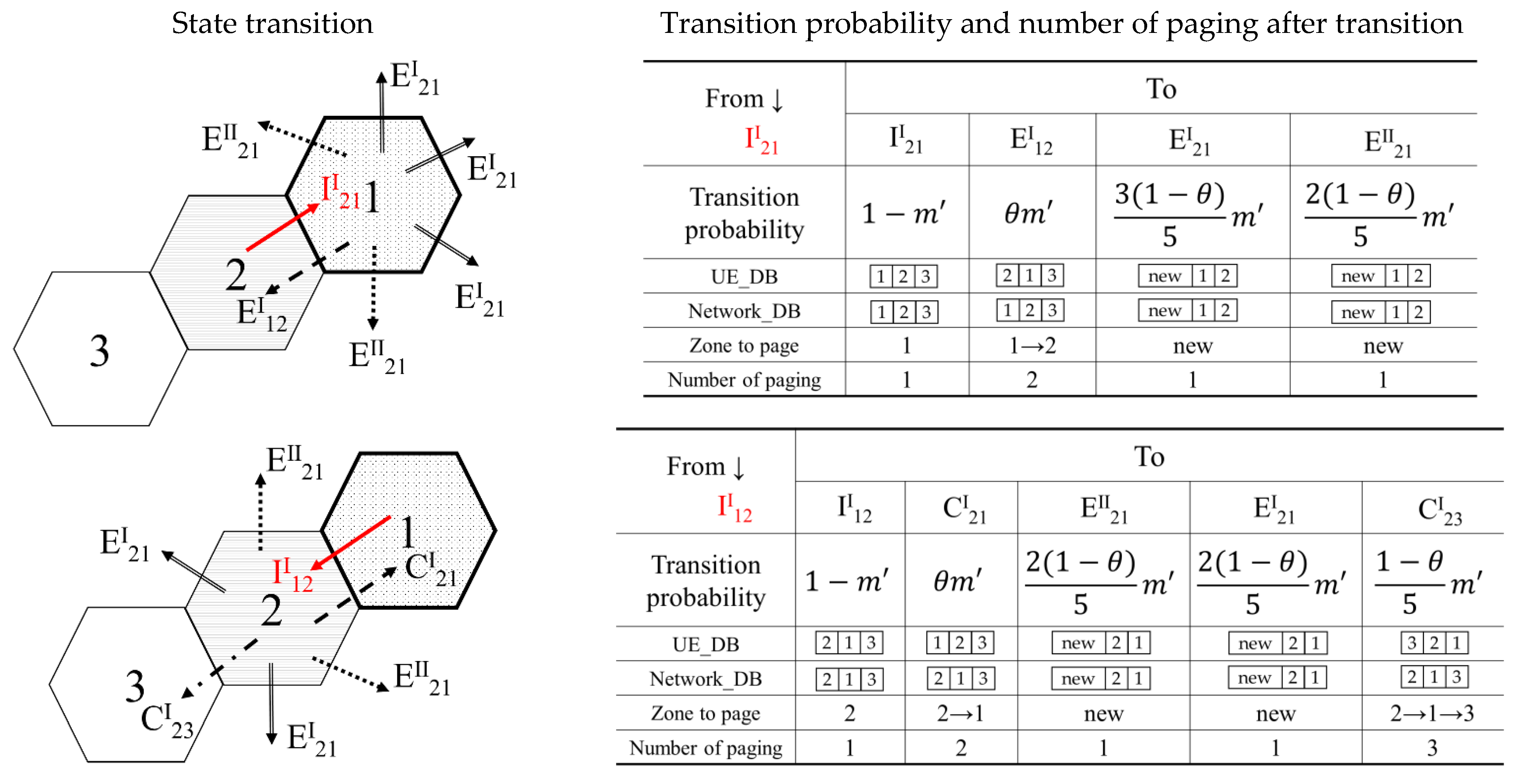
Figure 5 shows the transition probability to a feasible state, the zone number to be paged, and the number of paging procedures needed when an incoming call arises after changing to each state. To illustrate this point, the transition case from state
to other states is described as follows.
(i) : The UE moves from 3→2→1 and Network_DB has
. When the implicit registration is processed after the UE moves from zone 2 to zone 1, the Network_DB will not change. If an incoming call arrives before moving to another zone with a probability of 1 − m, one paging procedure is performed to find the UE in zone 1.
(ii) : UE can move to state if it returns to zone 2 with a probability of θm. When an incoming call arrives while the UE is staying in zone 2, the first zone 1 is selected from the Network_DB =
. As a result, there is no response. Thus, an extra paging procedure is required to find the UE in zone 2.
(iii) : The probability that the UE will move to another zone and then transit to state constituting a new serial-shaped RA (Type I) is 3(1 − θ)m/5. To connect the incoming call after shifting to , one paging is processed in the new zone where the UE has moved.
(iv) : The probability that the UE can transit to state is 2(1 − θ)m/5, thus constituting a new cluster-shaped RA (Type II). One paging is needed to find the UE while remaining in the new zone.
Similarly, for states defined in Type I, changeable states, transition probabilities between states, paging zones, and the number of paging procedures can be obtained, as shown in
Figure 5.
2.1.2. Case 2: Processing Implicit Registration inside Serial-Shaped RA
Figure 6 shows the state transition probability and paging procedure for two states (
and
). We also assumed that the UE moved from 3→2→1 and that Network_DB stored
. State
represents the state in which the implicit registration is processed after the UE moves from zone 2 to the edge area (zone 1 or 3). Similarly,
defines the state in which implicit registration is performed after the UE moves from the boundary to the middle zone (zone 2). The transition process from state
typically includes the following states:
(i) : If implicit registration occurs after UE moves from zone 1 to 2 in the middle, the Network_DB will be changed to
. With the arrival of an incoming call before moving to another zone, UE can be found in zone 2 through one paging procedure. The transiting probability to is 1 − m′.
(ii) : UE can enter state with a probability of θm′ if it returns to zone 1 after an implicit registration in zone 2. Two paging operations (2→1) are required for an incoming call after arriving at this state.
(iii) : The probability that the UE will make a new RA of Type II, that is, the transition probability from state to , is 2(1 − θ)m′/5. To connect an incoming call in the newly registered zone, one paging procedure is necessary.
(iv) : UE can move to state with a probability of 2(1 − θ)m′/5 if it constructs the new RA of Type I. An incoming call connection in the new zone is possible at once.
(v) : When the UE moves to zone 3 from zone 2, it moves to state with a probability of (1 − θ)m′/5. Since Network_DB is
, three paging procedures (2→1→3) in total are performed to locate UE in zone 3.
2.1.3. Case 3: Moving Three Zones after Call Occurrence in the Second Zone
After the UE moves from 3→2→1 and performs call processing in zone 2 while returning back to the zone, the Network_DB stores the middle zone 2 as the most recently registered area and the remaining zones at both ends in RA. In this case, four states are defined, as shown in
Figure 7. Representatively, the state transition process for the state of
can be described as follows. The
indicates a state in which the Network_DB has
after implicit registration in zone 2. The UE then moves from zone 3 to zone 2.
(1) : If a call occurs before the UE moves from zone 2 to another zone, it moves to state , and the probability is 1 − m. After converting to state , the Network_DB will become
, and one paging will be performed when connecting UE in zone 2.
(2) : UE can transit to state with a probability of θm when it returns to zone 3. The call connection in zone 3 requires three paging procedures (2→1→3).
(3) : The probability of configuring the new RA of Type I is 2(1 − θ)m/5. One paging arises to connect a call in the new zone.
(4) : When UE moves from zone 2 to zone 1, it transits to state . The probability is (1 − θ)m/5. Since the Network_DB is
, two paging operations are needed to find the UE staying in zone 1.
(5) : UE can enter state if it constructs a new RA corresponding to Type II, in which case the transition probability becomes 2(1 − θ)m/5. With the arrival of an incoming call in the new zone, one paging is processed.
2.2. Type II: Clustered Shape
Similarly, for Type II, the state definition and transition probability between states can be explained as follows.
2.2.1. Case 1: Moving inside 3Z after Forming a Clustered-Shape
In Type II, since it is a clustered-shape RA, there are three parts in contact between zones. Therefore, six states are defined according to UE’s movement between zones, as shown in
Figure 8. The case of the transition from
to other states is described as follows. Here,
refers to a state in which the UE moves from the most recently registered zone 1 to the second stored zone 2.
(i) : If the UE sends an implicit registration after moving to zone 2 and before moving to another zone, its state changes to and the probability becomes 1 − m. After implicit registration, the Network_DB will be newly updated to
, and the UE can be found through one paging procedure in zone 2.
(ii) : The transition probability to state corresponding to Type II is θm + (1 − θ)m/5. In this case, the UE returns to zone 1 or moves to a new zone to form a cluster-typed RA. In both cases, it can be seen that an incoming call connection is possible with one paging process.
(iii) : When the UE moves to zone 3, since Network_DB is
, three paging procedures (1→2→3) are required for an incoming call in zone 3. The state transition probability of → is (1 − θ)m/5.
(iv) : UE can move to state with a probability of 3(1 − θ)m/5 if it configures the new RA of Type I. The incoming call connection in the new zone is achieved through one paging process.
2.2.2. Case 2: Processing Implicit Registration inside Clustered-Shaped RA
If an implicit registration occurs in Type II, it is sufficient to define only the transition from
to other states, as shown in
Figure 9. After the UE moves from 2→1 and processes the implicit registration, the Network_DB becomes
, at which point the transition process from state
includes the following states:
(1) : When a call occurs in zone 1, the UE’s state becomes again (Network_DB =
). If an incoming call occurs while staying in zone 1 before moving to another zone with a probability of 1 − m′, one paging procedure is required.
(2) : UE can transit to state with a probability of θm′ if it returns from zone 1 to zone 2. Since Network_DB is
, two paging processes (1→2) are required to set the call in zone 2.
(3) : The UE can move to a new zone and form a serial-shaped RA of Type I. A new registered zone is stored in the Network_DB (
) with a probability of 3(1 − θ)m′/5. With the arrival of an incoming call, one paging procedure is performed in the new zone.
(4) : The UE’s state changes to with a probability of (1 − θ)m′/5 if it moves from zone 1 to zone 3. Three paging procedures (1→2→3) are requested using Network_DB =
in zone 3.
(5) : If the UE constructs a new cluster-shaped RA, its state changes to with a probability of (1 − θ)m′/5. One paging procedure is processed for an incoming call occurring in the new zone that has been moved.
In the following section, we will describe the method of computing a signaling cost for mobility management (registration and paging) on a radio frequency based on the transition probability between each state, as explained in
Figure 5,
Figure 6,
Figure 7,
Figure 8 and
Figure 9.
3. Modeling and Performance Analysis
As described in the previous section, 17 states are defined for two types and three cases. The following state transition matrix (P) can be obtained using the transition probability between states.
Note that the sum of the transition probabilities from each state to other states is 1. In a typical case, it can be confirmed that the sum of transition probabilities from
to other states (
,
and
) is 1
). The steady-state probability (
π) of each state can be obtained using
P in Equation (5) and the Markov chain method [
26]. However, since the time staying in each state differs for each case, it is necessary to compute an accurate steady-state probability by applying the semi-Markov process theory [
26] as described in the following subsection. Note that a Markov process considers transitions between states, determining future state probabilities based solely on the current state. On the other hand, a semi-Markov process incorporates both state transitions and the time taken for transitions, modeling the time required to reach future states alongside state transitions.
3.1. Sojourn Time and Exact Steady-State Probability
According to the semi-Markov process approach [
26], the steady-state probability of the UE should be recalculated using
π and the sojourn time spent in each state. First, for Cases 1 and 3, the sojourn time
and
of remaining in each state are expressed as follows.
Thus, we have the average sojourn time as follows:
Note that if a call occurs while the UE stays in the zone, the sojourn time is
. If the call does not occur, the sojourn time is
. Unlike Case 1 or 3, the sojourn time under Case 2 with the implicit registration connection is presented as follows:
That is, when a new call happens again before entering another zone after implicit registration,
If no call happens while entering another zone, it becomes the remaining residence time (
) in the zone. The mean sojourn time for Case 2 becomes as follows:
Therefore, the product
of the steady-state probability and the sojourn time can be defined as follows:
Here, we can obtain the steady-state probability
from the following balance equations and normalization conditions using the usual Markov chain [
26]:
Finally, the exact steady-state probability can be obtained as follows:
3.2. Registration and Paging Cost
The following symbols are used to compute the registration and paging cost:
U: Unit cost required to process one location registration procedure
Cu: Registration cost incurred during unit time for each UE
V: Unit cost of handling one paging per zone
Cp: Paging cost incurred during unit time for each UE
Ct: Total cost for registration and paging per unit time for each UE (Ct = Cu + Cp)
First, the registration cost per UE during unit time
can be given as follows:
where
A is the set of states for boundary zones in each RA, and
is the probability that the UE moves from state j to a new zone to request registration. For instance, in state
, if UE moves to a new zone in a manner that requires registration, as shown in
Figure 5, and its state changes to
or
, it is then registered with a probability of (
where
It should be noted that if the UE requests registration while moving, then that situation corresponds to the case where Network_DB stores the most recently registered zone as
as shown in
Figure 5,
Figure 6,
Figure 7,
Figure 8 and
Figure 9.
In the 3Z system, three selective paging procedures are assumed. The paging cost incurred for each UE during unit time is obtained as follows:
where
B is a total set of 17 states, and
is the average number of paging procedures in state
j for an incoming call. That is, the average number of paging procedures until the next call occurrence for each state can be calculated by multiplying the steady-state probability and number of paging processes, as depicted in
Figure 5,
Figure 6,
Figure 7,
Figure 8 and
Figure 9.
Finally, the total cost under the 3Z system can be obtained as follows:
4. Numerical Results
In consideration of a realistic operational environment, the following parameters are used to compare the performances of the 1Z, 2Z, and 3Z systems:
When
μ = 1, the time residing in each zone follows an exponential distribution with an average of 1.
Table 1 and
Figure 10 show the results for the three systems (1Z, 2Z, 3Z) while assuming
. As presented in
Table 1, as CMR increases, that is, as the time spent in the zone increases, the registration cost decreases, after which the total cost decreases. The results for hexagonal zones showed that the 3Z outperformed the 1Z and 2Z and that the cost of 3Z was always less than the cost of 1Z. The results also showed that if the UE stayed in the zone for a long time, that is, if the CMR was large, the improvement was reduced compared to 1Z or 2Z. However, the performance of 3Z was still the best.
Figure 10 shows the total cost and the relative cost reduction ratio. The left part of the vertical axis in
Figure 10 represents the total cost, and the right part indicates the cost reduction ratio (
red. ratio). The
red. ratio refers to the 2Z cost reduction ratio and the 3Z cost reduction ratio to the total cost of 1Z, respectively.
Figure 10 implies that as the CMR decreased (as the zone residence time decreased), the cost reduction ratio of the 3Z (or 2Z) system increased compared to that of the 1Z system.
Table 1 also shows the results for square-shaped zones (1Z_4, 2Z_4, 3Z_4) while assuming
θ = 1/4. The results showed that, in general, 3Z was better than 2Z in zone-based registration with hexagonal zones, and 2Z was better than 3Z in zone-based registration with square-shaped zones. Then, which performance was better, 3Z or 2Z_4? As shown in
Table 1, in the environment assumed in this paper, it could be seen that 2Z_4 was slightly superior for CMR = 0.25 and CMR = 0.5, while 3Z was slightly superior for CMR = 1, 2, and 4. In conclusion, it can be seen that the hexagonal zone might be superior, or the square-shaped zone might be superior depending on the network environment. Note that the difference was not significant.
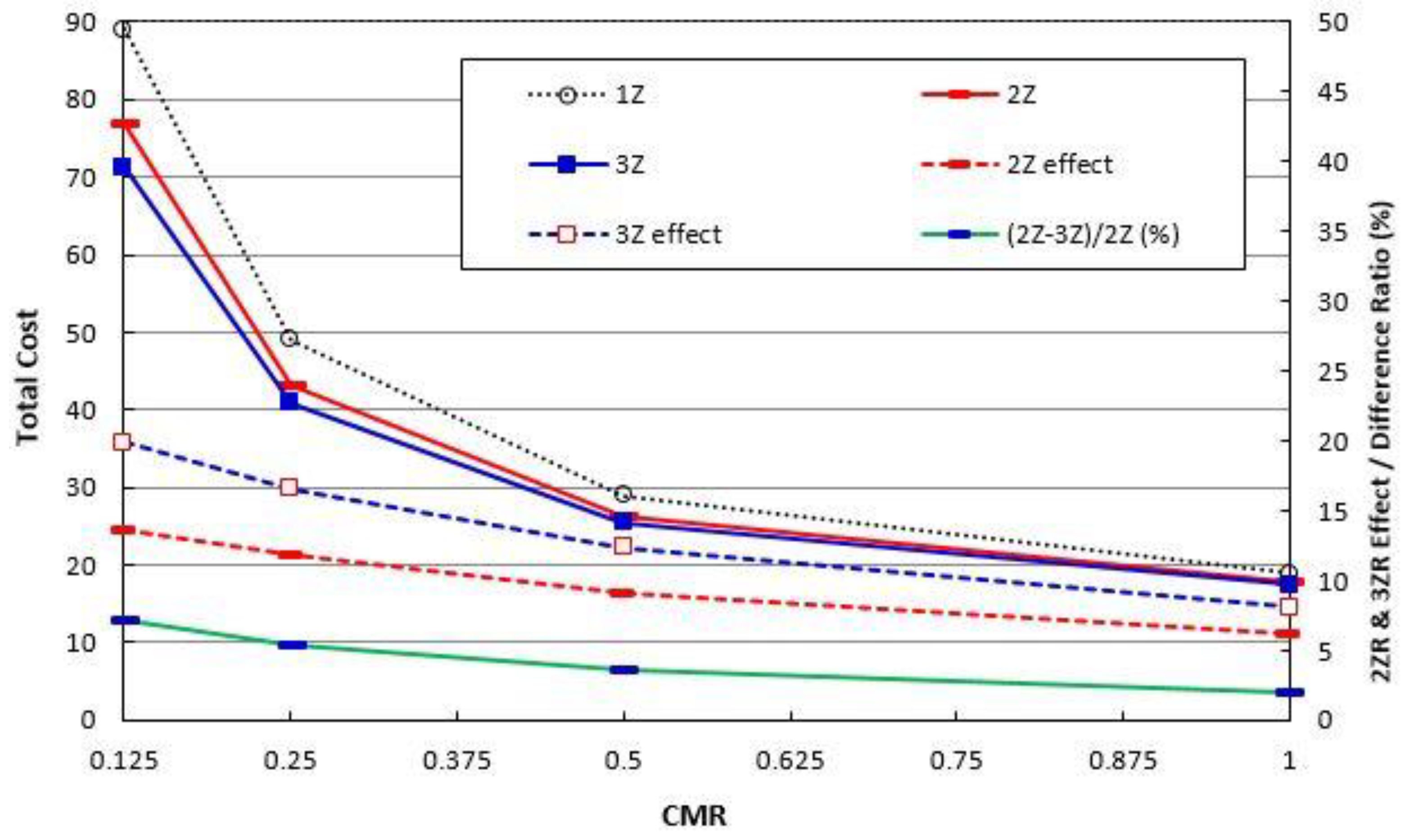
The analytical results for CMR < 1 are shown in
Figure 11. In the figure, the 2Z effect =
, the 3Z effect =
, and the
red. ratio of 3Z to 2Z are separately indicated. We could see that if CMR < 1, the cost at 3Z was always smaller than the cost at 1Z or 2Z. The smaller the CMR, the higher the reduction ratio.
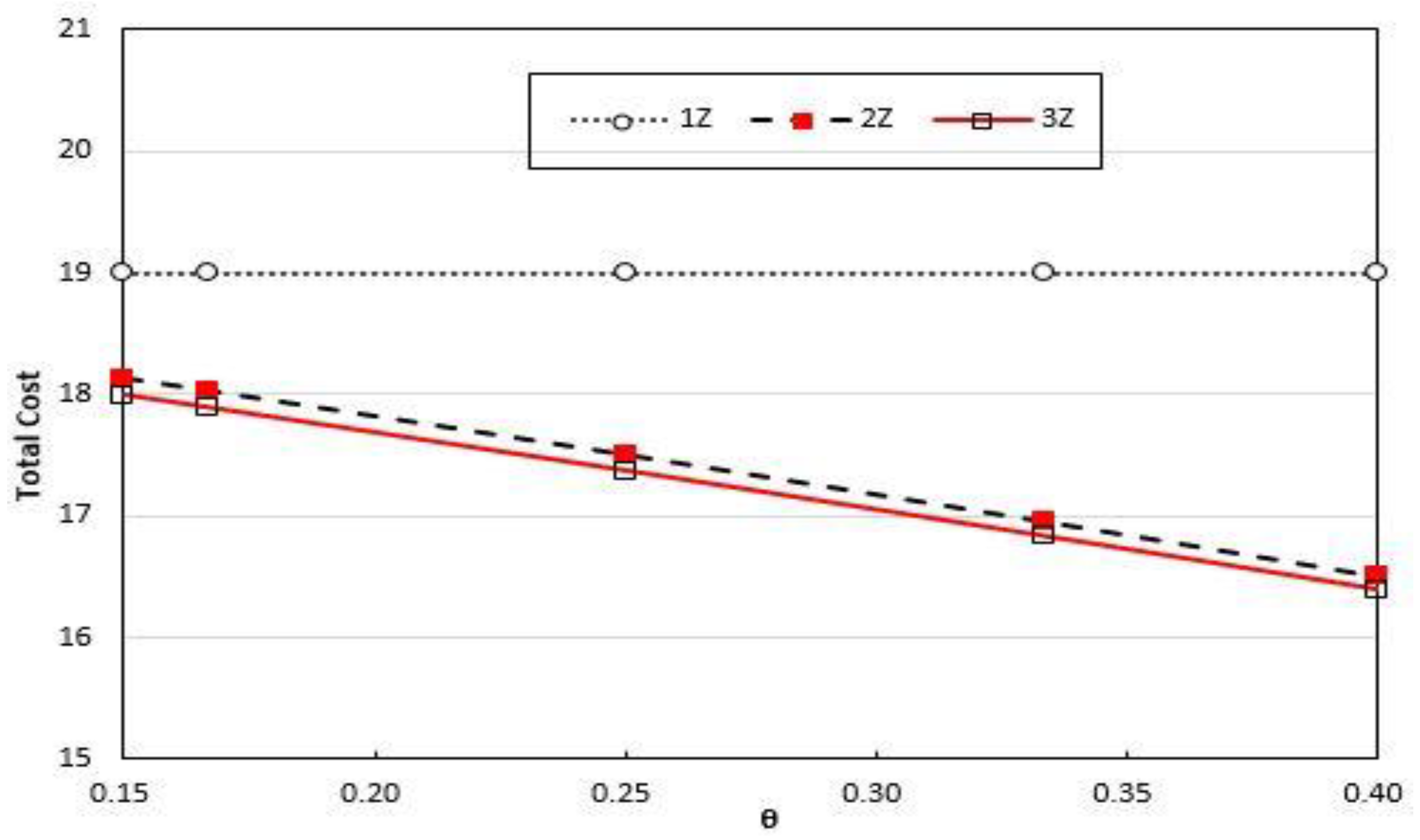
Figure 12 compares the total costs for various values of
. As a natural result, the 1Z system incurs costs regardless of
. The results revealed that in the 2Z or 3Z systems, as
increased (that is, as the probability of returning to previous zone increased), the registration cost decreased, after which the total cost decreased linearly.
Figure 13 and
Figure 14 show the registration and paging costs constituting the total cost as a function of
μ (the number of times entering the zone during unit time), respectively. As shown in
Figure 13, as
μ increased, the residence time in the zone decreased, and the registration cost therefore increased linearly. However, since 3Z manages three zones (two zones in 2Z) within one RA, the registration cost is always less than 1Z. On the other hand, as shown in
Figure 14, it could be seen that the paging cost to connect the UE increased as
μ increased. These results imply that the Network_DB does not know the exact zone of the UE, after which extra paging costs are incurred.
Figure 14 also showed that as
μ increased, the paging cost at 2Z and 3Z gradually increased due to the two-step paging in 2Z and three-step paging in 3Z, which was slightly reduced compared to the cost of one-step paging.
Based on the numerical results, we obtained the following major observations.
- (i)
The performance of 3Z improved more as the CMR became smaller; that is, when the UE traveled more in other zones.
- (ii)
For most CMR values, the 3Z outperformed the 1Z and the 2Z. The smaller the CMR, the better the performance of 3Z.
- (iii)
The greater the probability of returning to the previous zone, the more the performance of 2Z and 3Z could be linearly improved.
- (iv)
As the number of times entering another zone increased, that is, as the zone residence time decreased, the registration costs of 2Z and 3Z were smaller compared to the registration cost of 1Z by managing three or two zones with one RA.
- (v)
In 1Z, the paging cost was determined regardless of the UE’s zone residence time. However, in 2Z or 3Z, the paging cost gradually increased as the zone residence time decreased.
5. Conclusions
This study presented a new mathematical model for 3Z system with three zones among zone-based registration methods using a semi-Markov process approach. Assuming a hexagonal zone, the performance of 3Z was compared with those of previous 1Z and 2Z systems. That is, different from other previous studies, in this study, we analyzed performances of 1Z, 2Z, and 3Z for a hexagonal-shaped zone for the first time by exactly modeling two types of 3Z structures in more realistic wireless network environments. Based on the numerical results, when the call-to-mobility ratio (CMR) is smaller (that is, when the number of inter-zone movements of the user equipment (UE) is relatively high compared to the UE’s call occurrence), the performance of 3Z is more superior to 1Z and 2Z. Moreover, as the probability of returning to the zone previously registered increases and the number of times it moves to other zones increases, the registration cost eventually decreases, resulting in the better performance of 3Z. However, when the CMR is large (in this study, in the situation where the UE remains in the zone for more than twice the time interval of the call occurrence), the performance of 3Z is superior to that of 1Z and similar to that of 2Z. Finally, it was observed that efficient radio resources could be operated if the zone-based registration scheme was applied differentially in consideration of UE’s mobility (CMR). The results of this study can be used to design the optimal zone-based registration operation for each UE. The 3Z system can be easily implemented without substantial hardware development using the 1Z scheme that is widely used in most wireless communication networks.
The 3Z system is also be expected to be an algorithm to efficiently control movement of devices such as autonomous vehicles, drones, robots and moving IoT that will appear in 5G/6G networks in the future. Future studies should present a new model with improved performance by automatically configuring 3Z RA without needing additional registration using prior information on the zone id structure when the UE moves. Moreover, a comparative analysis could be conducted with previous studies, considering a square-shaped zone.


 : Registration,
  : No registration).
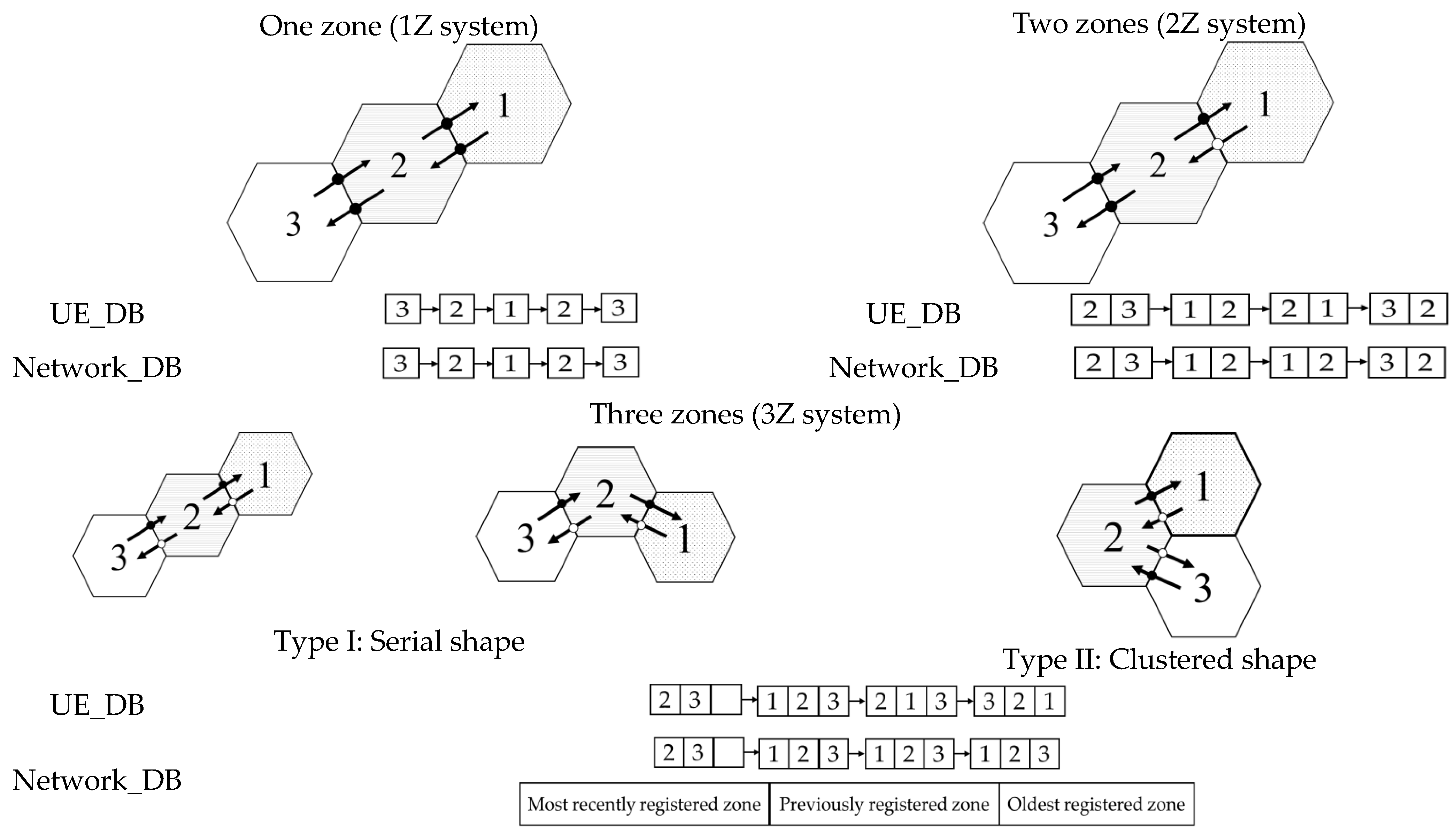
 : Call occurrence). (a) Type I; (b) Type II.


