Study on the Optimization of Pile Length of Micropiles in Soil Landslides

Abstract

This study summarizes the engineering design and calculation methods of micropiles and proposes a pile length optimization model based on numerical simulation software. Based on the proposed micropile calculation method and optimization method, a specific analysis of a project example was carried out, and a series of calculations, such as micropile design calculation and pile length optimization for the project, was completed. The results show that the miniature pile length optimization model based on numerical simulation finite difference method improves the previous method by automating the optimization process through fast modeling, automatic creation of optimization commands, and output and analysis of optimization results, and realizes the optimization of pile length using numerical simulation, which improves the efficiency of the optimization of the pile length under the premise of guaranteeing accuracy, and achieves the unity of both efficiency and accuracy. The feasibility of this optimization process is proved by engineering examples. The engineering practicability of the micropile design calculation method and optimization method proposed in this study is proved through practice. It provides a reference value for the initial fast and flexible management of small landslides.

1. Introduction

Landslides in China, as a common geological disaster, are characterized by fast movement, extensive range of destruction, and a strong impact on regional economic development [1]. For example, on 12 August 2015, a large landslide disaster occurred in Menggou Village, Zhongcun Town, Shanyang County, Shaanxi Province, resulting in 38 deaths, 1 injury, and 27 houses buried with extremely heavy losses [2]. On 23 July 2019, a landslide disaster occurred suddenly in Shuicheng County, located in Liupanshui City, Guizhou Province, resulting in 21 houses being buried, 1600 people affected, 9 missing, and 43 deaths [3]. Landslides in China are common geological disasters that move quickly, cause extensive damage, and hinder regional economic development.

In the 1950s, Lizzi in Italy proposed the micropile technology for foundation reinforcement. In the early 1970s, the Italian patent on micropile technology was terminated, and micropile technology saw real development internationally [4]. Over the past six decades, micropile technology has gained increasing recognition within the engineering community, evolving from its humble beginnings as a small-scale solution to its current status as a widely promoted and utilized technique. Bednarczyk et al. [5] evaluated the effectiveness of a variety of management methods, including micropiles, applied to manage landslides in the Polish Carpathians, showing that in most areas, micropile management solutions were effective. Macklin et al. [6] presented a case study of a micropile support scheme applied to a landslide remediation project, which served as temporary stabilization measures.

With the continuous research on miniature piles, the research on the response of miniature piles under seismic dynamic action has gradually become a hot topic. Many scholars have studied the response characteristics and deformation law of micropiles under dynamic loads through numerical simulations or related shaking table tests and centrifugal shaking table tests. Aomar Benslimane et al. [7] summarized their research on the dynamic characteristics of micropiles in sandy soil foundations under seismic loads using centrifugal model tests and pointed out that the fundamental frequency of micropiles is affected by the arrangement form. The monopile’s base frequency is affected by its arrangement, and this frequency is closely linked to the inclination angle of minipile arrangements. When minipiles are arranged in rows, they provide stronger resistance against seismic loads while experiencing smaller bending moments and bearing displacements compared to regular piles under similar vibratory loads.

In the numerical simulation of seismic dynamics, Chuanyou He [8] established three numerical models of micropiles with different inclination angles using numerical simulation software to investigate the working performance of micropiles in liquefied sites under self-weight conditions and seismic action and derived the approximate distribution locations of the maximum bending moment of micropiles under seismic action and the variation law of pile top displacement with seismic wave intensity.

Based on the results of numerical simulations, scholars have also made relevant suggestions for the seismic calculation of miniature piles. Yang Jing [9] adopted the numerical analysis tool to investigate the problems related to micropiles under dynamic loads and derived the dynamic response characteristics of micropile-reinforced slopes and the seismic calculation method of micropile combination structures based on the amplification factor method. However, the dynamic soil pressure law on the pile side derived from the simplified analytical model lacks verification through relevant shaking table tests or actual measurement data.

For the study of pile length, Poulos [10] found that when the length of the embedded section of the minipile is insufficient, the horizontal resistance of the soil below the slip surface reaches its ultimate value, and the minipile as a whole undergoes rigid motion with the landslide. Vigianil [11] investigated the correlation between the peak moment and embedment ratio (the ratio of the embedded section to the length of the loaded section) of piles and derived a critical embedment ratio for lateral rigid movement. This critical value represents when piles undergo lateral stiffness movement.

He Hui [12] studied the embedment depths of 1/4, 1/3, and 2/5 pile lengths in pile swelling soil landslide prevention and control by physical model tests, and the results showed that the foot slope and pile top displacement tend to decrease as the embedment depth increases, and the embedment depth of a 1/3 pile length is more suitable.

Zhu Yong [13] et al. used the strength discount finite element method to analyze several factors affecting the stability of slopes reinforced by anti-slip piles and obtained the optimal design elements of anti-slip piles, such as optimal pile position and critical pile length, which provide a reference basis for the optimal design of a row of piles and established the deformation prediction mathematical model, which provides a reference basis for the deformation control of the pile body. In order to reduce or eliminate the deformation of high-speed railroad foundation bulge, Chen Weizhi [14] et al. carried out the actual engineering cases and designed key parameter research studies based on the wet–dry test of the Yungui Railway foundation bed and improved the traditional minipile into a kind of anti-uplift long and short minipile structure. It is recommended to use “small pile diameter, small pile spacing” long and short micropiles to reinforce the ballasted railroad foundation base expansion soil. Liao Lijian [15] et al. proposed a linked iterative algorithm for pile length optimization under seismic loading, which accurately calculates the optimal pile length for friction pile foundation of bridge abutment and provides a reference for the optimal design of pile foundation structure for railroad bridges. Yu Gui [16] et al. took gray soil pile reinforcement of large quasi-heavy railroad roadbed as the engineering background and researched the influence of factors such as pile shaft inclination, pile diameter, pile distance, and pile length on the effect of gray soil pile reinforcement of existing railroad roadbed with the help of finite element software. It provides a theoretical basis for the engineering design and safety evaluation of gray soil pile-reinforced existing railroad roadbeds. Wang Weiyu [17] et al. applied large-scale finite element numerical analysis software to establish a numerical analysis model based on the field model test and under the condition of basic assumptions. Upon adjusting the parameters of pile length in the pile raft foundation, the pile length was optimized. Based on numerical simulation software, Mengfei Qiu [18] et al. set up a numerical model for mechanical analysis to select the reasonable location of multiple rows of anti-slip piles and compare the design parameters of Rizheng software with collected data to determine the optimal values of pile spacing and anchoring depth and apply them to the engineering examples for verification. The analysis concludes that this optimization design method is feasible and practical and can provide a reference for subsequent landslide management. You, C. [19] et al. optimized the structural parameters of h-type anti-slip piles using numerical software, which showed that the optimum beam stiffness was three times the front and rear piles, the optimum rear pile depth was 0.28 times the length of the rear pile, and the depth of the front pile was 0.5 times the length of the front pile. Benmebarek, M.A. [20] et al. performed numerical calculations using PLAXIS 2D and 3D to optimize a row of piles in cohesive friction slope reinforcement. The results show that fixed pile heads located in the middle of the slope provide better stability and reduce the optimum length of the piles. Xu, C. [21] et al. proposed a new multi-objective comprehensive optimization method for the optimization problem of anti-slip pile reinforced slopes and analyzed the effects of pile position, pile length, and pile spacing on the reinforcing effect of homogeneous slopes through numerical simulation. A large number of scholars have conducted research in pile length optimization. Most of them study the pile length optimization problem of anti-slip piles, multi-row piles, and bridge piles; although some scholars have also studied the pile length [22] optimization problem of micropiles, the pile length optimization problem of micropiles must still be further researched, and this study improves the pile length optimization problem of micropiles, so that small landslides can be managed economically and quickly, and the loss of life and property caused by landslides can be prevented and reduced.

When dealing with landslides, it is important to clarify the load-sharing mechanism of each row of micropiles and the load-carrying mechanism of individual micropiles. Based on this, this chapter summarizes and derives the design calculation method of minipiles in order to obtain a more convenient and practical engineering design calculation method. At the same time, the pile length design problem that was not directly solved using the previous model experiments and numerical simulations was optimized using engineering structural optimization ideas so as to truly solve the practical design problem of minipiles from an engineering perspective.

2. Methods

2.1. Micropile Design Calculation Method and Pile Length Optimization Study

When dealing with landslides, it is important to clarify the load-sharing mechanism of each row of micropiles and the load-carrying mechanism of individual micropiles. Based on this, this chapter summarizes and derives the design calculation method of minipiles in order to obtain a more convenient and practical engineering design calculation method. Simultaneously, the unresolved issue of pile length design in previous model experiments and numerical simulations was addressed through the application of engineering structural optimization principles, thereby effectively resolving the practical design problem of minipiles from an engineering perspective.

Numerous experts and scholars have extensively discussed the design and calculation methods of micropiles, including influential approaches such as the ultimate bearing capacity method, p-y curve method, Ding Guangwen method, and elastic foundation beam method, among others. From the 1970s to 1990s, Lizzi, Cantoni [23] and Juran et al. [24] proposed a design method for mesh minipile reinforced slopes, but this method relies heavily on subjective experience and judgment, and in China, Pei-Dong Shi and Kai-Sheng He et al. [25] also conducted related research and gave an empirical calculation formula foundation beam theory for the normal working phase and tensioning phase of anchors to establish a set of calculation models for the calculation of the interaction between this combined structure and the soil. This study optimizes previous design methods using a “global to local” analytical approach, providing a reliable and user-friendly analysis and calculation method for engineering applications.

Based on the phenomena and data analyzed in previous model tests and numerical simulations, micropiles within soil landslides exhibit deformation and failure characteristics similar to those of elastic piles. Furthermore, according to the current calculation theory in the code [26], the type of pile can be determined based on the deformation coefficient using the following equation (The definition of the deformation coefficient α is derived from the specification GB/T38509-2020 Landslide Prevention and Control Design Code [S] and is defined by the equation.):

$$\left\{\begin{array}{c}\alpha =\sqrt[4]{k{b}_0/4EI}\left(\mathrm{k}-\mathrm{law}\right)\\ \alpha =\sqrt[5]{m{b}_0/EI}\left(\mathrm{m}-\mathrm{law}\right)\end{array}\right.$$

(1)

Equation (1) calculates the type of pile based on the deformation coefficient, where k is the embedded section foundation coefficient, in the “k method” is a constant; m is the embedded section foundation coefficient scale factor, in the “m method” with the depth of z change and linear change; b₀ is the calculation width, for the miniature pile such as round small pile, generally take, b₀ is the width of the pile, b₀ is the width of the pile, b₀ is the width of the pile, b₀ is the width of the pile, b₀ is the width of the pile, in general take $b_0=0.9\left(1.5d+0.5\right)$, d is the diameter of the pile. d is the pile diameter. In practical engineering applications, taking the elastic modulus E as 3 × 10⁷ kPa (C30 concrete) and assuming the worst-case scenario for the embedded soil layer, taking m = 1000 kPa/m² and k = 3 × 10⁴ kPa/m, the relationship curve between the diameter of the micropile and the deformation coefficient shown in Figure 1 can be calculated. As illustrated in the figure, it can be observed that there is a decrease in the deformation coefficient with an increase in pile diameter for micropiles ranging from 0.09 m to 0.3 m; however, when using the product of the deformation coefficient α and the embedded length h₂ of the pile to determine the type of micropile (k method: rigid pile when αh₂ ≤ 1 and elastic pile when αh₂ > 1; m method: rigid pile when αh₂ ≤ 2.5 and elastic pile when αh₂ > 2.5), based on data shown in Figure 1, when the embedded length of the micropile exceeds 6 m (calculated using the “m method” for a pile diameter of 0.3 m), it can be regarded as an elastic pile regardless of the soil conditions, and this length can be achieved in practical engineering.

Micropiles can be considered elastic based on both experimental phenomena and engineering theoretical calculations. Therefore, the mature calculation theory of elastic piles can serve as a reference for calculation, forming the theoretical basis for the method described in this chapter.

As shown in Figure 2, first, multiple rows of micropiles and the soil between them are considered a whole, forming a combined anti-sliding system. The system is assumed to share the sliding force generated above the pile position, and then the force is distributed among the micropiles according to the ratio of sliding force that each pile can bear, which is determined by model tests and numerical simulations. Consequently, the consolidation of multiple rows of micropiles into a single row is undertaken for computational purposes. Subsequently, within a given calculation width, each individual micropile is segmented based on soil layers, and the ground coefficient method is employed to determine parameters such as pile displacement, bending moment, and shear force, among others, in each segment. Ultimately, reinforcement calculations are conducted based on the distribution of internal forces along the pile.

2.2. Calculation Method for Static Design of Micropiles

(1)

Determine the monopile load

According to the conclusions of the model experiments, it can be assumed that micropiles are elastic–plastic materials with a clear yield limit. Under the action of landslide thrust, the rear row of piles that directly resist the thrust will enter the yield stage first. Furthermore, the issue of pile length design, which was not directly addressed by previous model experiments and numerical simulations, was optimized using engineering structural optimization principles to effectively solve practical design problems related to minipiles from an engineering perspective. The specific calculation method is as follows:

①

Calculation of landslide thrust

The calculation of landslide thrust can be carried out using the simplified Bishop method or the transfer coefficient method according to the code [27], which will not be further elaborated here.

②

Thrust distribution

The thrust distribution is determined by taking a conservative distribution ratio based on the results of the static tests and numerical simulations mentioned earlier. The specific distribution ratios are determined according to

Table 1. Table of landslide thrust distribution coefficients.

Pile Position	Rear Pile	Middle Row Pile	Front Row Piles
Allocation ratio	0.411	0.348	0.241

. Data in Table 1 are derived from the previously conducted tests, and the landslide thrust was actually measured based on the pressure boxes arranged in the middle and back rows of piles before and after the tests, which ultimately resulted in the landslide inference coefficients [28].

(2)

Calculation of Pile Length

According to the relevant experimental results, it can be assumed that when the micropile is subjected to bending and shear, the pile body will shift from mainly bearing bending and shear to mainly bearing tensile and compressive forces after the pile body bends and cracks. Assuming this premise, if the pile body undergoes excessive deformation leading to plastic failure, the bending and shear resistance of the pile body will cease to increase. However, during the plastic deformation stage, the pile body still exerts a restraining effect on the soil above and below the sliding surface. Consequently, at this juncture, micropiles primarily endure tensile forces. However, with the increase in the tensile force, the micropile may experience a pull-out failure. In order to avoid such failure, the pile length of the micropile needs to be determined based on its anchoring characteristics. Referring to existing calculation theories, assuming the diameter of the micropile is D and the diameter of the longitudinal reinforcement in the pile is d, the pile length required for the micropile to meet the anchoring performance can be calculated according to Formula (2).

$$L=\max \left(\frac{K{f}_s{A}_s}{\pi D{q}_1},\frac{K{f}_s{A}_s}{n\pi d\xi q_s}\right)$$

(2)

According to the formula, K is the safety factor, which can be obtained from Table 8.2.2 in reference [27]; q₁ is the design value of the bond strength between the cement stone and the pile hole wall, which can be selected from Table 8.2.3-2 and Table 8.2.3-3 in reference [27]; q_s is the design value of the bond strength between the cement stone and the steel bar, which is 0.8 times the standard value and can be obtained from Table 8.2.4 in reference [27]; n is the number of steel bars; ξ is the reduction factor of the interface bond strength when multiple steel bars are used as longitudinal reinforcement, which can be selected from the range of 0.6 to 0.85.

By utilizing this approach, the anchorage length of micropiles in both the sliding bed and sliding body can be computed, thereby enabling the determination of Ld and Lu, respectively. Generally, the anchorage length of micropiles in the sliding body is equal to the thickness of the sliding body at the pile location h₁. When h₁ is less than Lu, the anchorage length in the sliding body is insufficient, and a connecting beam should be installed at the top of the pile for reinforcement.

(3)

Differential control equation for monopile by elastic coefficient method

For soil landslides, the m-method is commonly used to calculate the pile’s force using the elastic coefficient method. However, for some dense clay and stone-mixed soils, the k-method is sometimes used. Consequently, this study introduces two elastic pile calculation models, namely the “m-m method” and the “m-k method”, specifically tailored for soil landslides, with the aim of providing a valuable reference for the design and computation of micropiles in all types of soil landslide scenarios.

As shown in Figure 3, the total length of the micropile is H, with a loaded section length of h₁ above the sliding surface and an embedded section length of h₂ below the sliding surface. To ensure the universality of the sliding force distribution form, the sliding force shared on the micropile is assumed to have a trapezoidal distribution, with a load distribution degree of p0 at the pile top and a load distribution degree of pA at the sliding surface. When p0 = pA, it is a rectangular distribution, and when p0 = 0, it is a triangular distribution. The diameter of the micropile is d, and its bending stiffness is EI.

Based on the m-method and k-method in the specification, we integrate the procedures of m-method and k-method in the process of application and propose the m-method and m-k-method.

①

The “m-m” method

The “m-m” method treats the sliding bed soil and the sliding body soil equally and calculates both the upper and lower sides of the sliding surface using variable foundation coefficients. The foundation coefficient above the sliding surface is assumed to be k₁ = m₁y (m₁ is the proportionality coefficient of the foundation coefficient of the loaded soil layer). The foundation coefficient below the sliding surface is k₂ = k + m₂y (m₂ is the proportionality coefficient of the foundation coefficient of the embedded soil layer, and k is the foundation coefficient at the sliding surface). Then, as shown in Figure 2, under the combined action of the sliding force and soil resistance, the micropile undergoes bending deformation in its loaded section. The bending differential equation for the loaded section is:

$$EI\frac{d^{4}y}{d{z}^4}+b_0{m}_{1}zy=p_0+\left(p_A-p_0\right)\frac{z}{h_1}$$

(3)

The aforementioned equation is a fourth-order variable coefficient homogeneous differential equation, which can be solved through various methods such as the power series method, numerical integration method, and finite difference method. For the purpose of facilitating programming calculation, this study employs the finite difference method for solving the above equation.

When employing the finite difference method for solution, initially, the micropile is discretized into smaller segments, wherein the total length H is divided into n segments of length h, and subsequently assigning numerical labels to the nodes within each individual segment. For convenient programming calculation (to avoid negative and zero subscripts), as shown in Figure 3c, for the loaded section of the pile, the top node of the pile is numbered 3, the node of the pile at the sliding surface is numbered X, and two virtual nodes are set at both ends of the loaded section of the pile, numbered 1, 2 and X + 1, X + 2, respectively. Then, for any node i in the loaded section of the pile, the control difference equation is:

$$\frac{EI}{h^4}\left(y_{i-2}-4y_{i-1}+6y_i-4y_{i+1}+y_{i+2}\right)+b_0{m}_1\left(i-3\right)h{y}_i=p_0+\left(p_A-p_0\right)\frac{\left(i-3\right)h}{h_1}$$

(4)

The same holds true for the embedded pile segment below the sliding surface, which can be considered a horizontally loaded pile subjected to shear and bending moments at the pile head. The differential equation governing its deflection is:

$$EI\frac{d^{4}y}{d{z}^4}+b_0\left(k+m_{2}z\right)y=0$$

(5)

Using the same discretization approach as the loaded pile segment, as shown in Figure 3, for the embedded pile segment, the node at the pile bottom is numbered 3, the node at the sliding surface is numbered X′, and two virtual nodes are placed at both ends of the embedded pile segment, numbered as 1, 2 and X′ + 1, X′ + 2, respectively. The governing difference equation for any node j on the embedded pile segment can then be expressed as:

$$\frac{EI}{h^4}\left(y_{j-2}-4y_{j-1}+6y_j-4y_{j+1}+y_{j+2}\right)+b_0\left\{k+m_2\left[h_2-\left(j-3\right)h\right]\right\}{y}_j=0$$

(6)

②

The“m-k” method

The “m-k” method distinguishes between the sliding soil and the soil of the sliding body, employing the variable foundation coefficient method above the sliding surface and the constant foundation coefficient method below it. Let k₁ = m₁y be the foundation coefficient for the loaded soil segment above the sliding surface, where m₁ is the proportionality coefficient of the soil foundation coefficient; let k₂ be the foundation coefficient for the anchored soil segment below the sliding surface, which is a constant value. The differential equation governing the loaded segment is identical to that used in the m-m method Equation (3), and the same discretization approach is applied to the pile body, resulting in an equivalent difference equation for any node on the loaded segment as shown in Equation (4) of the m-m method.

Below the sliding surface, the embedded pile segment can be considered as a horizontally loaded pile subjected to shear and bending moments at the pile head, and its deflection differential equation is:

$$EI\frac{d^{4}y}{d{z}^4}+b_0{k}_{2}y=0$$

(7)

Similarly, by discretizing and numbering the embedded pile segment, the governing difference equation for any node j on the embedded segment can be expressed as:

$$\frac{EI}{h^4}\left(y_{j-2}-4y_{j-1}+6y_j-4y_{j+1}+y_{j+2}\right)+b_0{k}_2{y}_j=0$$

(8)

By differentiating the aforementioned control points and incorporating corresponding boundary conditions, as well as continuity conditions for internal forces, displacements, and rotations at the sliding surface, a recursive formula can be derived to iteratively solve for node displacement along the pile body. In order to save space in this chapter, the differential method for solving the displacement equation will be detailed in the subsequent algorithm implementation section.

(4)

Solution of Internal Forces in Micropiles

Based on the aforementioned difference control equation, the displacement of all nodes along the pile body can be calculated using a computer. The corresponding distributions of pile bending moment, shear force, and soil pressure can be obtained through the utilization of the subsequent recursive formula. Bending moment:

$$\mathrm{Bending} \mathrm{moment}: M_i=\frac{EI}{h^2}\left(y_{i+1}+y_{i-1}-2y_i\right)$$

(9)

$$\mathrm{Shear} \mathrm{force}: Q_i=\frac{EI}{2h^3}\left(y_{i+2}-2y_{i+1}+2y_{i-1}-y_{i-2}\right)$$

(10)

$$\mathrm{Earth} \mathrm{pressure}: {\sigma }_i=k{y}_i$$

(11)

In the equation, k represents the foundation coefficient. When the “m method” is used for calculation, k = mz; when the “k method” is used for calculation, k is a constant.

Therefore, utilizing the aforementioned method enables the resolution of internal force distribution and deformation in micropiles, which can be integrated with reinforced concrete structure design principles to facilitate corresponding micropile section design. It should be noted that when using this method for anti-sliding structure calculation, it is usually necessary to verify whether the calculated soil pressure is lower than the allowable compressive strength of the rock and soil body on the side of the pile.

2.3. Seismic Design Calculation Method of Micropile

Many feasible methods have been proposed by scholars in the industry for the seismic design calculation of micropiles, such as the time history analysis method, response spectrum method, pseudo-static method, etc. However, for multi-degree-of-freedom systems such as micropiles with complex stress states, it is virtually impossible to perform time history analysis and response spectrum analysis calculations without the use of numerical calculation methods. Therefore, the more traditional pseudo-static method is still recommended in engineering. To ensure the reliability and operability of the seismic design calculation method for micropiles described in this study, this study will also explore the seismic design calculation method for micropiles based on the pseudo-static method.

When the pseudo-static method is applied to the calculation of anti-slide structures, the seismic action is actually simplified to the product of the weight of the sliding body and the corresponding seismic coefficient, which is applied as the seismic force on the anti-slide structure to calculate the internal forces and deformations of the anti-slide structure. Essentially, by effectively simulating seismic force, this method enables a complete integration of seismic design calculation with static design calculation, allowing for direct application of the principles and methods of static design calculation in seismic design. Therefore, it can be known that under the vibration action, the thrust force of the loaded section of micropiles is closer to the trapezoidal distribution feature, and there is a more obvious load-sharing feature between each row of piles. Therefore, when dealing with a clearly defined dynamic load, the seismic design calculation for micropiles can be conducted using a method entirely consistent with the static design calculation. As a result, the focus of research on the seismic design calculation of micropiles is simplified to simulating the seismic force acting on them. According to the calculation results of the amplification coefficient in the vibration table test and numerical simulation, referring to the current seismic code [29], the recommended amplification coefficient of 2.25 is used to directly amplify the calculated static load, and the amplified thrust value is taken as the value of the load for dynamic calculation.

Table 2. Comparison table of dynamic load calculation of each row of micropiles (unit: kPa).

Item Pile Position	Test Results			Numerical Simulation Results
	Measured Static Load	Multiply the Amplification Factor	Measured Dynamic Load	Measured Static Load	Multiply the Amplification Factor	Measured Dynamic Load
Rear Pile	55.55	124.99	109.48	54.41	122.42	115.88
Middle row pile	47.05	105.86	100.44	53.6	120.60	87.00
Front row piles	32.68	73.53	41.02	35.53	79.94	67.30

displays a comparison table of the results obtained using the static amplification and dynamic calculation for each row of micropiles. In the table, the measured static load is the result of the static load under the critical failure load in the model test and numerical simulation. The measured dynamic load is compared with the peak acceleration of 0.6 g, which has been selected based on the bearing limit state of the rear row of piles. As can be seen from the table, the calculated load of each row of micropiles after being amplified by the static load is greater than the measured dynamic load. In the test, the static load of the rear row and middle row of piles after being amplified is relatively close to the measured dynamic load result, but because the load-sharing ratio of the front row piles measured in the vibration table test is relatively low, its result deviates significantly from the measured value after multiplying the static load by the amplification coefficient. In the numerical simulation, after calculating the load-sharing according to the maximum value of the loaded section, there is also some deviation between the measured dynamic load of each row of piles and the calculated value using the amplification coefficient method, with a smaller deviation for the rear row piles and relatively larger deviation for the middle and front row piles. However, overall, this deviation tends to be conservative, rendering it acceptable for engineering design purposes. Consequently, based on the results obtained from this test and numerical simulation, this calculation method can be deemed fundamentally reliable.

Considering the randomness of earthquake occurrence, this study suggests that in engineering practice, the seismic design calculation of micropiles should focus on verification. The verification process is similar to the static design process of micropiles. Compared to static design calculations, seismic design calculations can appropriately reduce the safety factor in order to balance engineering safety and economy. The specific value of the seismic design safety factor should be referenced from relevant structural seismic codes.

2.4. Optimization of Micropiles Length Based on Numerical Simulation

2.4.1. Mathematical Model for Pile Length Optimization

Based on the previous discussion on the design calculation method of micropiles, it is evident that precise design calculations for the cross-section of micropiles can be achieved by employing thrust sharing theory and elastic foundation beam theory. However, when determining the length of micropiles, only anchorage requirements have been taken into account. Experimental results indicate that the anchoring characteristics of micropiles gradually manifest as they approach failure. Therefore, the length of micropiles determined solely based on anchorage requirements obviously has great potential for optimization. Thus, it is necessary to conduct optimization design research on the length of micropiles to improve the design theory and method of micropiles.

The pile length optimization design proposed in this study is a type of structural optimization design. Generally speaking, structural optimization is the process of solving the variables to be optimized under given design parameters, satisfying the constraints, and obtaining the optimal solution of the objective function. Its mathematical model includes the following aspects:

(1)

Design Variables

In the optimization process, it is often necessary to first specify the design values of some parameters and then adjust the values of other design parameters to achieve the optimization goal. These adjustable design parameters are called design variables. For the micropile length optimization carried out in this study, the design variable is set as the length of the micropiles, denoted as PL. Then we have:

$$PL=[P{L}_1,P{L}_2,\cdots P{L}_n]$$

(12)

Where denotes the length of the first row of micropiles along the direction of landslide movement, denotes the length of the second row of micropiles, and so on up to the nth row of micropiles.

(2)

Objective Function

The objective function, sometimes called the performance function, is an index used to measure the goodness of the design solution. In this study, the optimization objective function is PL_max − PL_min ≤ ε to screen out the optimal length of pile length, which represents the cost of construction. Optimization means selecting the best pile length that meets the conditions by algorithm under the premise of satisfying the safety factor so as to reduce the cost of the project.

The mathematical relationship between the objective function and the design variables is calculated using a reasonable geotechnical constitutive model and the finite difference method, which will be described in detail later in the study.

(3)

Constraints

Constraints are necessary conditions for obtaining a convergent solution in optimization design. The pile length optimization carried out in this study needs to satisfy the following two constraints:

①

The constitutive equation, boundary conditions, and initial conditions are required for the finite difference solution of the micropile treatment landslide model.

②

The range constraint of the design variable, which is the length of the micropile, needs to be satisfied.

The value of the design variable should meet the condition: $P{L}_{\min }\le PL\le P{L}_{\max }$. In which $P{L}_{\min },P{L}_{\max }$ represent the upper and lower bounds of the design variable pile length, respectively. Calculations will be performed by the design method of minipiles.

③

The constraint function is determined as the stability safety coefficient of the slope after the micropile treatment, denoted as Fos. Different from the conventional optimization design method, using the safety coefficient as the index for evaluating the design scheme is not to obtain the maximum value of it as the design objective but to set a specification-allowed safety coefficient [Fs] index as the lower limit of the constraint objective function. That is, the reasonable solution must be satisfied for pile length optimization (The factor of safety is obtained by strength discounting method in numerical simulation.):

$$Fos\ge [F_s]$$

(13)

2.4.2. Optimize Process Analysis

The optimization problem in this study is to determine the safest pile length using our optimized mathematical model. The optimization process will include two main modules: theoretical calculations and numerical calculations. The specific implementation steps are as follows:

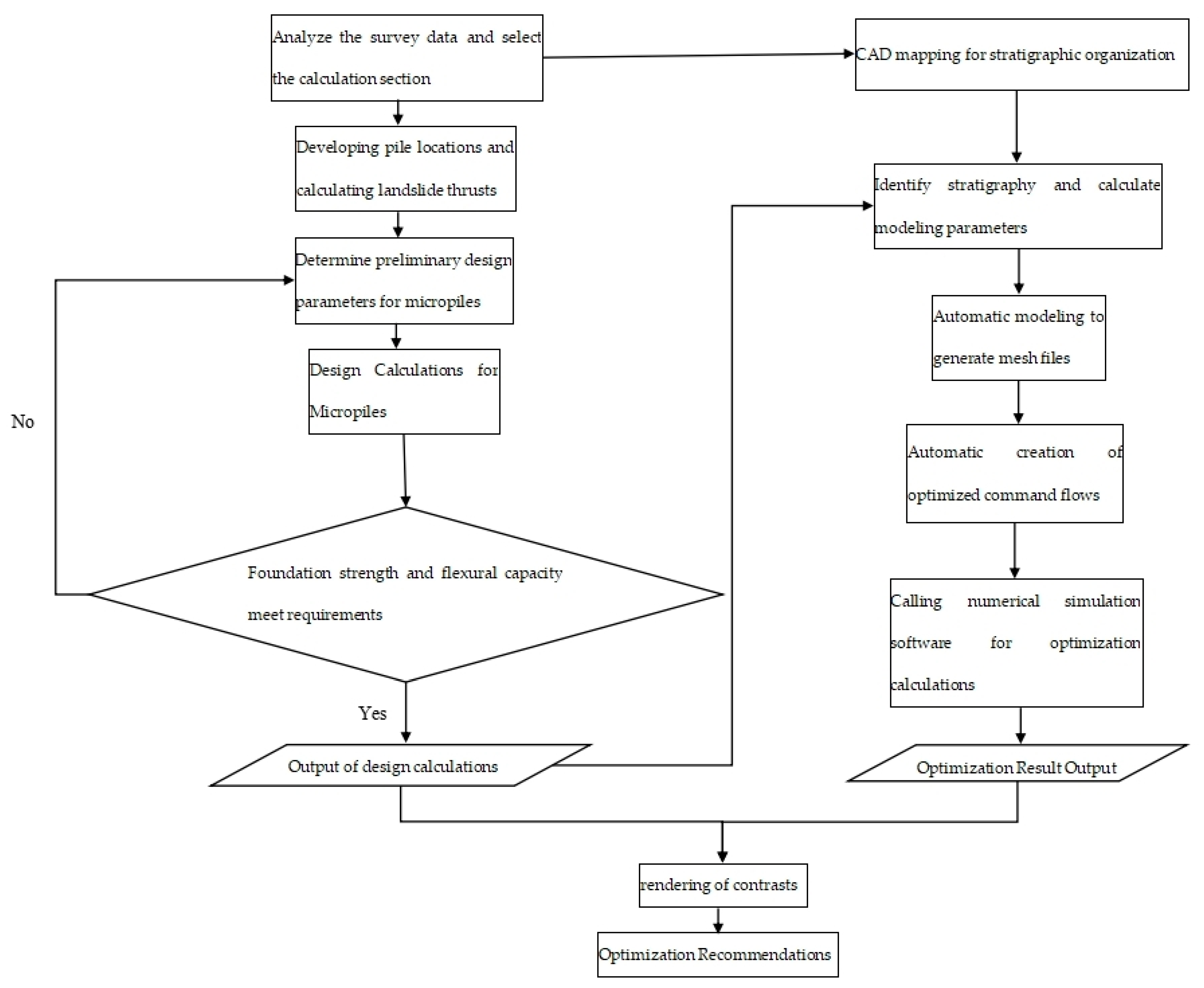
Step 1: Analyze the landslide survey data, determine the calculation section of the landslide, and complete the related profile CAD drawings. Step 2: Determine the pile layout and calculate the landslide thrust. Step 3: Prepare the preliminary design parameters of the pile, such as pile diameter, spacing, length, material, foundation coefficient, stratum parameters, and calculation mode. Step 4: Calculate pile displacement, internal force, earth pressure, and pile length according to the calculation method described in Section 1. Step 5: Verify the foundation strength and micropile flexural bearing capacity. If satisfied, continue with Step 6. If not, return to Step 3. Step 6: Draw the internal force distribution and displacement maps of the pile and provide reinforcement suggestions. Step 7: Based on the CAD drawings obtained in Step 1, organize the stratum lines and save them as a CAD exchange file format “.dxf”. Step 8: Read and identify the stratum line exchange file, calculate the model’s size parameters, and determine the modeling parameters and boundary parameters based on the calculation results. Step 9: Automatically create and mesh the numerical simulation grid and output the grid file. Step 10: Automatically create the numerical simulation command flow file for optimization calculations. Step 11: Call numerical simulation software for numerical optimization calculations and iterate for different pile lengths. Step 12: Read and analyze the optimization calculation results and provide optimization suggestions. The optimization flow chart is shown in Figure 4.

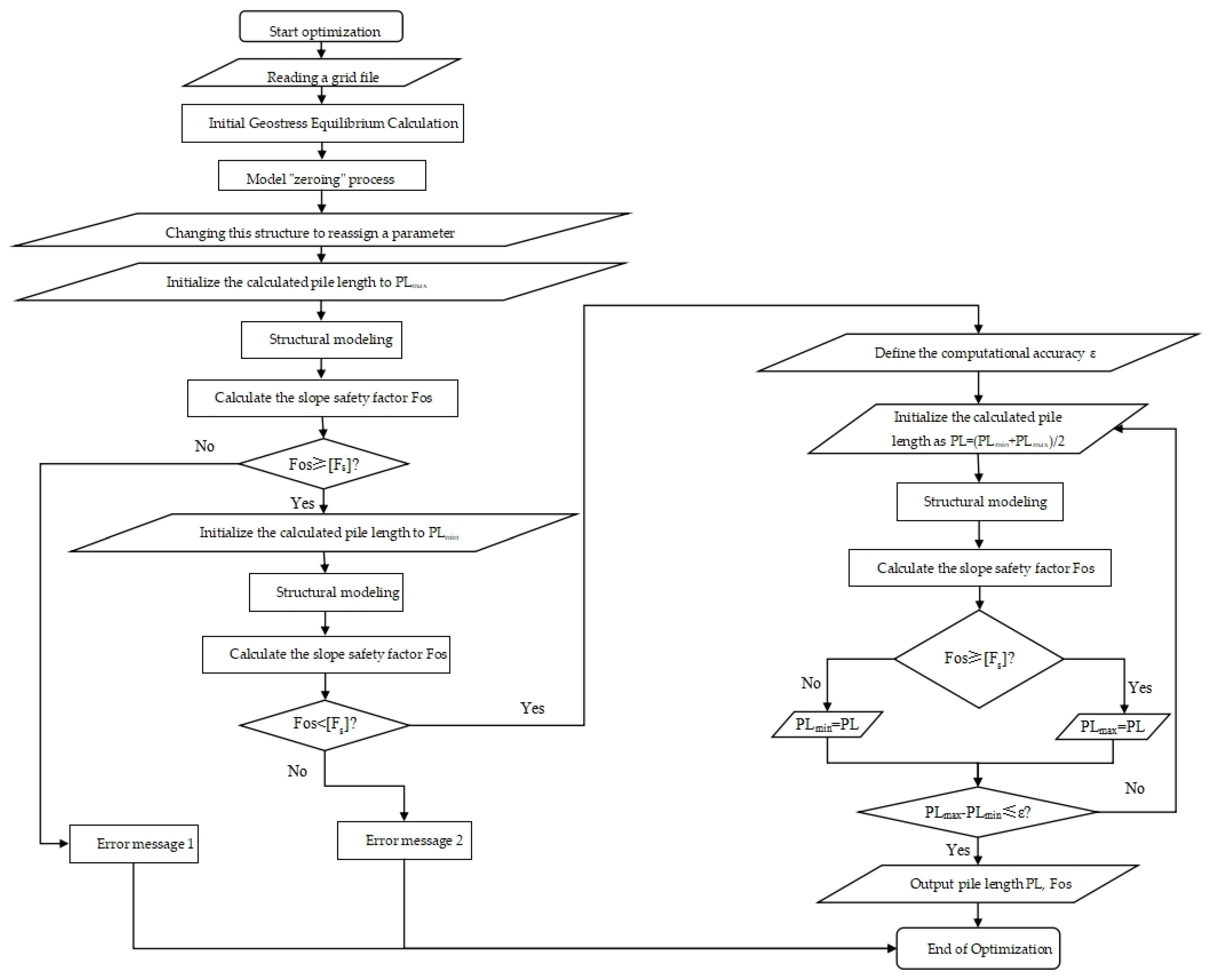
In particular, the optimization command flow file created in Step 10 includes the core algorithm of the entire optimization process, including the following procedural steps:

S1: Read the model grid file output by Step 9. S2: Perform initial stress equilibrium calculations: define the constitutive model as an elastic model; assign calculation parameters to all strata; create a contact surface between the sliding body and the sliding bed and assign parameters to the contact surface; further set boundary conditions and apply gravity, and calculate until convergence is reached. S3: “Zeroing” the model after initial stress calculations (eliminating displacement and plastic zones). S4: Change the soil constitutive model to the Mohr–Coulomb model and assign calculation parameters. S5: Structured modeling of micropiles and connecting beams (or plates) at the pile locations and assign structural calculation parameters. The pile length used in this modeling is the calculated pile length in Step 4, which is the upper limit of the design variable PL_max. S6: Set boundary conditions and calculate the slope safety factor after micropile reinforcement under self-weight working conditions. If the safety factor is not less than the allowable safety factor [Fs], proceed to the next step. Otherwise, it prompts an error message stating that the pile length design is deemed unreasonable or the simulation parameters are not set reasonably. Please review and attempt again. The flowchart of the optimization algorithm for micropile length is shown in Figure 5.

(Note: the reason for triggering Error Prompt 1 is that when using the design calculated pile length PL_max for modeling and calculating, the safety factor is too low, indicating that the design pile length is too small to guarantee the landslide control effect, or there are problems with the numerical simulation of the strata parameters, resulting in unsafe numerical simulation calculation.)

S7: Reset the pile length to the lower limit PL_min. PL_min is taken as the construction length if there are no special requirements, i.e., PL_min is the sum of the bearing segment pile length and the embedded segment pile length. The embedded segment pile length is generally taken as one third of the full pile length and not less than 4 m in construction design. After determining PL_min, rebuild the structure model, assign parameters, and calculate the safety factor. If the safety factor is still less than the allowable safety factor [Fs], proceed to the next step. Otherwise, it gives an Error Prompt 2: The minimum pile length already meets safety requirements, and no optimization is needed. Please check if the input parameters are reasonable.

(Note: Error Prompt 2 is triggered when the safety factor meets the requirements after modeling and calculating with the design calculated pile length PL_min, indicating that the minimum pile length already meets the safety requirements and there is no room for pile length optimization. However, it is also possible that there are problems with the numerical simulation of the strata parameters, leading to a risky numerical simulation calculation.)

S8: Set the optimization calculation accuracy ε. S9: Set the pile length PL = (PL_max + PL_min)/2, rebuild the structure model again, and calculate the safety factor. If the safety factor is less than the allowable safety factor, then set PL_min = PL; if not, set PL_max = PL. S10: Compare the difference between PL_max and PL_min. If it is not greater than the set accuracy ε, output the optimization results. Otherwise, return to S9. Continue the optimization process until the desired level of calculation accuracy is achieved, and subsequently present the optimized results as output.

2.4.3. Programmatic Implementation of Optimization Algorithms

(1)

The programmatic implementation of the micropile theory calculation method relies on the solution of the difference control equations.

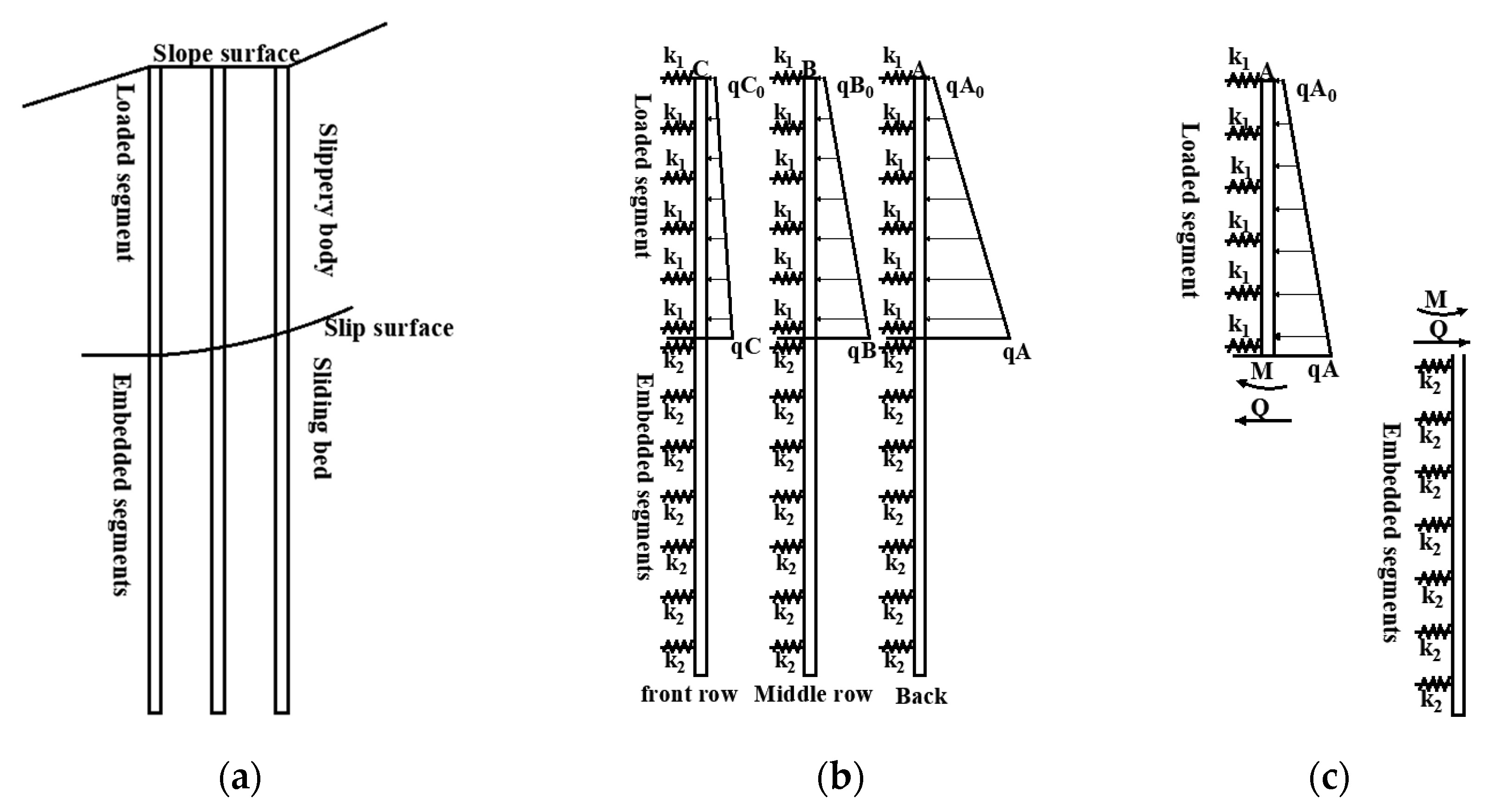
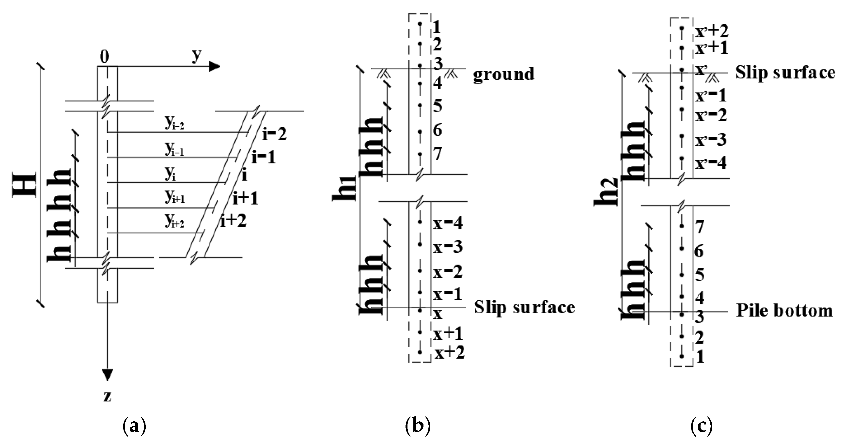
The key to implementing the theoretical calculation method for micropiles lies in solving the differential control equation. The specific approach is to derive the corresponding recursive formula and its parameter values from the boundary of the pile body from both ends. Then, the current equation group is formed with the continuity condition near the sliding surface, and the node displacement near the sliding surface is solved, which is gradually diffused to the entire pile length to complete the solution of the displacement equation. To optimize space utilization, we present the recursive equations for parameters and node displacement in both “m-m” and “m-k” methods based on the differential calculation model depicted in Figure 3. These equations can be readily programmed for solution. The specific derivation process will not be repeated.

①

The “m-m” method

(a)

Parameter recursive formula for the loaded section:

Initial value: $a_1=nan$, $b_1=nan$, $c_1=nan$; (This initial value is not involved in the operation and is used here as a placeholder for nan);

$$\begin{array}{c} a_2=2, b_2=1, c_2=0;\\ a_3=2, b_3=1, c_3=q_0{h}^4/EI;\\ \mathrm{Recursion}:d_i=a_{i-2}{a}_{i-2}-b_{i-2}-4a_{i-1}+6+b_0{m}_1(i-3)h^5/EI;\\ a_i=\left(a_{i-2}{b}_{i-1}-4b_{i-1}+4\right)/d_i; b_i=1/d_i;\\ ci=\left\{\frac{h^4}{EI{h}_1}\left[q_0{h}_1+\left(q_A-q_0\right)\left(i-3\right)h\right]-a_{i-2}{c}_{i-1}-c_{i-2}+4c_{i-1}\right\}/d_i\end{array}$$

 

In the formula $i\in [4,h_1/h+5]$, refer to the previous section for the meaning of other parameters.

(b)

Recursive formula for embedded segment parameters:

Initial value: $A_1=nan$, $B_1=nan$, $C_1=nan$; (This initial value is not involved in the operation and is used here as a placeholder for nan);

Considering various forms of support at the base, there are corresponding alterations in the initial value. The specific values are shown in

Table 3. Table of initial values of parameters.

Type	Pile Bottom Free	Pile Bottom Hinge Support	Pile Bottom Fixation
Sequence 2 takes the value	$A_2=2$, $B_2=1$, $C_2=nan$	$A_2=2$, $B_2=1$, $C_2=nan$	$A_2=2$, $B_2=-1$, $C_2=nan$
Sequence 3 takes the value	$A_3=4/C_3$, $B_3=2/C_3$, $C_3=2+\left(K+m_2{h}_2\right)b_0{h}^4/EI$	$A_3=0$, $B_3=0$, $C_3=nan$	$A_3=0$, $B_3=0$, $C_3=nan$

Note: In the equation, nan is a placeholder, not involved in the operation, K is the foundation coefficient at the slip surface, taken as: $K=m_1{h}_1$.

below:

Recursion: $C_j=A_{j-2}{A}_{j-1}-B_{j-2}-4A_j-1+6+\left\{K+\left[m_2{h}_2-\left(j-3\right)h\right]\right\}{b}_0{h}^4/EI$;

$B_j=1/C_j$; $A_j=\left(A_{j-2}{B}_{j-1}-4B_{j-1}+4\right)/C_j$;

In the formula $j\in [4,h_2/h+5]$, refer to the previous section for the meaning of other parameters.

Based on the continuity conditions of displacement, rotation, bending moment, and shear force at the sliding surface position of the micropile, combined with the recursive calculation equation derived from Equation (6), the following linear equation group can be obtained by taking the five points near the sliding surface as shown in Figure 3: X − 2, X − 1, X, X + 1, X + 2:

Displacement continuity: $y_X=y_{X\prime }$

Continuous cornering: $y_{X+1}-y_{X-1}=-\left(y_{X\prime +1}-y_{X\prime -1}\right)$

Shear continuity: $-y_{X-2}+2y_{X-1}-2y_{X+1}+y_{X+1}=y_{X\prime -2}-2y_{X\prime -1}+2y_{X\prime +1}-y_{X\prime +2}$

Continuous bending moment: $y_{X-1}+y_{X+1}-2y_X=y_{X\prime -1}+2y_{X\prime +1}-2y_{X\prime }$

Recurrence formula for the loaded section: $y_X=a_X{y}_{X+1}-b_X{y}_{X+2}+c_X$

$y_{X-1}=a_{X-1}{y}_X-b_{X-1}{y}_{X+1}+c_{X-1}$

$y_{X-2}=a_{X-2}{y}_{X-1}-b_{X-2}{y}_X+c_{X-2}$

Recursive formula for embedded segments: $y_{X\prime }=A_{X\prime }{y}_{X\prime +1}-B_{X\prime }{y}_{X\prime +2}$

$y_{X\prime -1}=A_{X\prime -1}{y}_{X\prime }-B_{X\prime -1}{y}_{X\prime +1}$

$y_{X\prime -2}=A_{X\prime -2}{y}_{X\prime -1}-B_{X\prime -2}{y}_{X\prime }$

A set of ten equations is provided, which can be solved to determine ten unknown displacement variables. Then, according to the corresponding recursive formula, the displacement values of all nodes of the micropile can be iteratively obtained, and the internal force of the micropile and the soil pressure can be further calculated.

②

The “m-k” method

The main difference between the “m-k” method and the “m-m” method is that the former uses a constant foundation coefficient in the embedded section of the pile. Based on the “m-m” method derivation results mentioned above, the recursive outcomes of embedded section parameters reflect the primary discrepancy between the two calculations. For the “m-k” method:

(a)

Parameter recursive formula for the loaded section:

Initial value: same as the “m-m” method;

Recursive: same as the “m-m” method;

(b)

Parameter recursive formula for the embedded section:

Initial value: $C_3=2+k{b}_0{h}^4/EI$, the rest are the same as the “m-m” method;

Recursion: $C_j=A_{j-2}{A}_{j-1}-B_{j-2}-4A_j-1+6+b_{0}k{h}^4/EI$; the rest are the same as the “m-m” method;

In the formula $j\in [4,h_2/h+5]$, refer to the previous section for the meaning of other parameters.

The continuity condition and recursive equation at the sliding surface for the “m-k” method are identical to those of the “m-m” method, while the solution approach remains essentially unchanged. This will not be reiterated herein.

The m-method and k-method are based on the code to determine the deformation characteristics presented under the action of landslide thrust, i.e., whether it is a rigid or elastic anti-slip pile. This directly affects the form of distribution of soil pressure at the embedded end. The distribution form of earth pressure is determined by the type of judgment through the actual parameter calculation, and the distribution form of the finite element model is determined by the actual force form. Then, the m-m method and m-k method are used to screen out the optimal pile length, which is applied in the finite element model.

(2)

Numerical simulation rapid modeling

Numerical simulation rapid modeling technology is the key to the finite difference solution used in the optimization method in this study. In order to achieve the engineering operability of the optimization process, modeling work must be fast, convenient, and easy to master. Therefore, this study designs an automated rapid modeling algorithm for numerical simulation from section to model and briefly introduces this module.

①

CAD graphics recognition and processing

In order to facilitate programming processing, the dxf file used as the input of the model section shape needs to meet certain drawing specifications, including ① The graphics should only contain section stratigraphic lines, slope lines, and sliding surface lines without any other extraneous graphic elements; ② All lines are single lines; ③ In order to facilitate the program to identify the function of the line, different stratigraphic lines should be distinguished by relative line widths, with the sliding surface line being the thinnest, followed by the slope line, and the other stratigraphic lines gradually increasing line width according to the decrease in their elevation.

The dxf file format is essentially a text file, which records information such as the starting point, ending point, and line width of the line in the form of keywords. It is easy to extract these key information through programming and classify their functions according to the line width specifications mentioned above so as to obtain the coordinate information of various types of lines in the section.

②

Plane modeling and coordinate adaptation

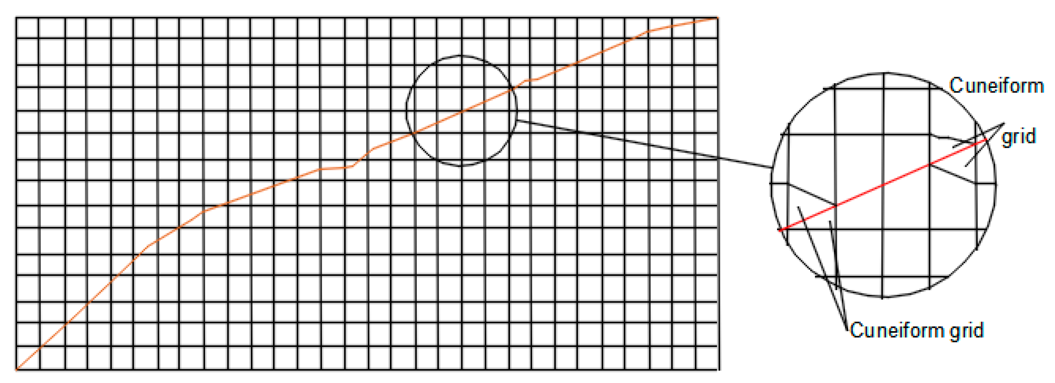
Plane modeling is based on the coordinate information extracted from CAD graphics recognition. As shown in Figure 6, for an irregular stratigraphic line, a rectangular grid is established to completely cover the stratigraphic line. The size of the rectangular grid can be controlled by input variables, which is also the basic grid size of the model. After the plane modeling is completed, in order to make the model grid adapt to changes in the terrain, the coordinates of the grid are offset nearby, as shown in the enlarged schematic diagram in Figure 6. In this manner, trapezoids or triangles are employed to substitute the initial regular rectangular grids in proximity to the stratigraphic line, thereby enabling the grid to conform with the stratigraphic line.

By applying this method to process all the stratigraphic lines in the model, corresponding sectional grid divisions can be obtained, which provides a foundation for subsequent 3D stretching modeling. It should be noted that the plane coordinate and coordinate adaptation algorithm are critical components throughout the modeling process. After this process is completed, the quality of the model grid usually needs to be manually checked. In cases where the slope line is steep but increasing grid quantity is not feasible, local irregularities may arise at the contact between strata. To address this issue, stretching the x-coordinate during dxf graphics processing can be employed to achieve a gentler slope. After the modeling is complete, the x-coordinate can be restored through the “ini xpos multiply” command.

③

3D Stretching and Node Generation The plane grid model obtained from the previous step is stretched and expanded to form a three-dimensional space coordinate with multiple layers from the plane coordinates. After being stretched, the three-dimensional coordinates of all points become the most basic elements of the numerical simulation model-node coordinates.

④

Unit Composition and Grouping numerical simulation units are composed of nodes. For hexahedral elements, there are eight control points named p0, p1...p7. The positions of these eight points must conform to the “right-hand rule” and cannot be arbitrarily reversed. The composition of numerical simulation units is to arrange the serial numbers of these eight nodes in the prescribed order and assign a unit number to them. For the mesh nodes obtained by the aforementioned plane modeling and stretching, most of them can form hexahedral elements. However, for a small number of cases where the stratigraphic line passes through a quadrilateral mesh, as shown in Figure 6, it needs to be split into two triangles. The construction of two wedge-shaped elements for smooth grouping of the model is limited to only the nodes located on both sides of the stratigraphic line. In the program implementation, once the relative position between the unit-forming nodes and the stratigraphic line is recognized in programming, it becomes straightforward to identify these nodes requiring division into wedge-shaped elements and accomplish unit composition for the entire model.

After the unit composition, the constructed units can be grouped according to the stratigraphic boundaries. For ease of operation, the geometry geological interface grouping technology built into numerical simulation is used for rapid grouping. Specific operations can refer to the numerical simulation technical manual.

After completing these four key steps, it is possible to directly generate a numerical simulation calculation model from the profile map. With corresponding programming operations, this process has a high degree of automation and can achieve one-button modeling. This rapid modeling technology also overcomes the complex obstacles of modeling for optimization solving using the finite difference method with numerical simulation software.

(3)

Generation of numerical simulation calculation commands

To further ensure the engineering feasibility of the optimization program and reduce the difficulty of writing numerical simulation optimization command streams for different landslide forms and parameters, command streams that can be used for optimization calculations are automatically generated. Based on the calculation results mentioned earlier and the parameter transmission, this study uses an Excel spreadsheet to assign basic numerical simulation parameters and then reads these data through a program, combining the results of parameter transmission to generate numerical simulation calculation command streams for initial stress balance calculation, initial slope stability calculation, and pile stability calculation.

(4)

Analysis and presentation of optimization results

The optimization solution process described in the previous section obtains a table of corresponding pile lengths and safety factors. After achieving convergence, the internal forces of the pile can be extracted and analyzed under the optimal working condition corresponding to the converged solution, facilitating automatic graph generation. This result is the internal force distribution result obtained by numerical simulation analysis. In practical operation, it can be compared with the results obtained by theoretical calculation, and if necessary, the larger value can be taken as the design value of the structural internal force.

2.4.4. Example Analysis

The selected example is a typical landslide behind a plant in the northwest region, with a slope width of about 160 m, a length of about 95 m, and a height difference of about 32 m between the front and the back edge. Slip material for the original slope area of the slope surface residual slope deposits and the overlying Loess landslide form is more obvious, with a slope of about 15°~25°. According to survey data, the stratigraphic parameters are taken as shown in

Table 4. Table of surveyed stratigraphic parameters.

Serial Number	Stratigraphic	Modulus of Elasticity/MPa	Ck (kPa)	Φk (°)	Γ (kN/m3)	Poisson’s Ratio
1	Sliding Body	20.0	23.84	19.18	19.2	0.32
2	Q4del Stacking layer	20.0	24.10	20.12	19.2	0.32
3	Red clay	25.0	27.83	20.95	19.6	0.30
4	Pebble and gravel layer N22	30.0	34.25	22.15	19.8	0.27
5	Claystone N21	40.0	42.04	23.65	19.8	0.25
Sliding surface		—	15.3	14.6	—	—

. The characteristic period of the ground vibration response spectrum within the project area is 0.35 s, with a design basic seismic acceleration value of 0.15 g and corresponding seismic intensity at level VII.

According to the stability calculation based on the parameters provided by the survey, the results show that the stability safety coefficient of the slope body is only 1.03 in the natural state, less than 1.0 in the saturation condition, and less than 1.05 in the earthquake condition. Its stability level is poor, and engineering treatment is urgently needed. Considering the relatively modest annual rainfall in the project area and favorable natural drainage conditions surrounding the slope, achieving full saturation becomes challenging. Therefore, engineering calculations are conducted using parameters representative of the natural state.

According to the calculation profile and stratigraphic parameters provided by the survey, the landslide thrust is calculated using the transfer coefficient method recommended by the code, and the landslide thrust at the proposed pile location is about 548.64 kN/m (the safety factor is taken as 1.2). The load-sharing ratios obtained under static and dynamic working conditions can be calculated separately to obtain the load-sharing table, as shown in

Table 5. Load sharing table.

Pile Position	Rear Pile	Middle Row Pile	Front Row Piles
Share ratio	0.411	0.348	0.241
Load sharing (kN/m)	225.5	190.9	132.2

.

Based on the landslide form and thrust level of the treatment project, the engineering design proposes utilizing a minipile group for landslide remediation. As shown in Figure 6, three rows of minipiles with 0.15 m pile diameter, 1.5 m pile spacing, and 1.4 m row spacing are used in a plum-shaped arrangement.

In order to simplify the engineering calculation and reduce the construction difficulty, the same design section is used for the three rows of piles, and the maximum thrust force is p = 225.5 kN/m. It is assumed that the thrust is triangularly distributed for the design calculation of the minipile and the calculation method is based on the calculation theory in Section 1, and the “m-m” method is used. The values of foundation coefficients are taken as shown in

Table 6. Table of values of foundation coefficients.

Stratigraphic	Q4del Stacking Layer	Red Clay	Pebble and Gravel Layer N22	Claystone N21
Foundation factor m(kPa/m2)	3500	5000	9000	12000

below.

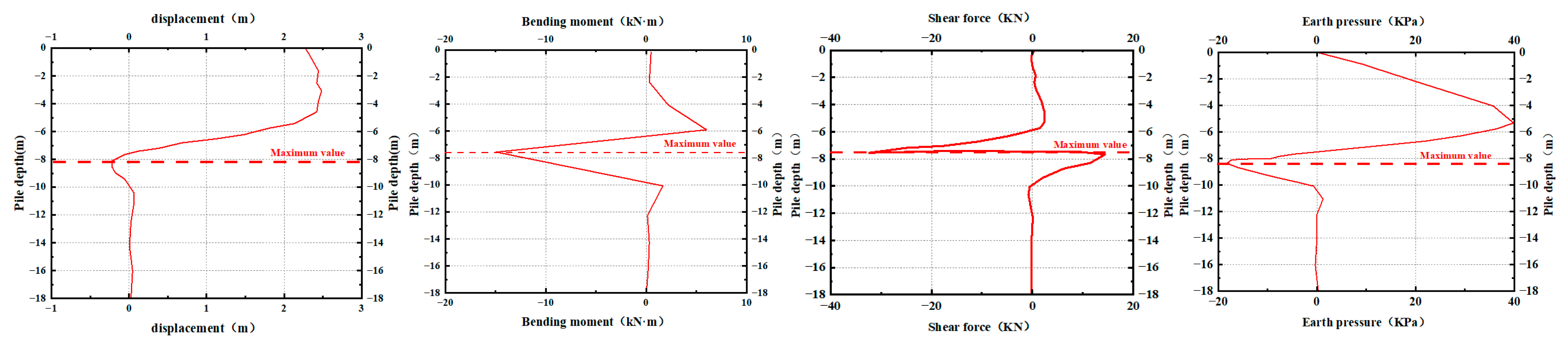
The calculation assumes a fixed pile bottom, and the determined length of the pile is based on empirical evidence to ensure that the minipile can penetrate the clay rock layer by at least 3 m, which is temporarily set as 18 m in this study. The calculated displacement, internal force, and earth pressure curves are shown in Figure 7.

From the figure, it can be seen that the maximum bending moment is about 15.44 kN·m, and the maximum shear force is about 35.25 kN, from which the reinforcement calculation is carried out. In order to facilitate the construction, a steel pipe concrete minipile is used for this minipile, so according to the Technical Specification for Steel Pipe Concrete Structure (GB50936-2014) [30], Q235 steel pipe with 152 mm outer diameter is used and C30 fine stone concrete is injected inside, according to the wall thickness was calculated to be about 2.7 mm according to the requirements of bending shear resistance, so the steel pipe specification was selected as φ152 mm × 3 mm.

According to the calculation results in the previous section, the optimal design is carried out with PL_max = 18 m, PL_min = 10 m, and setting the allowable safety factor [Fs] = 1.40.

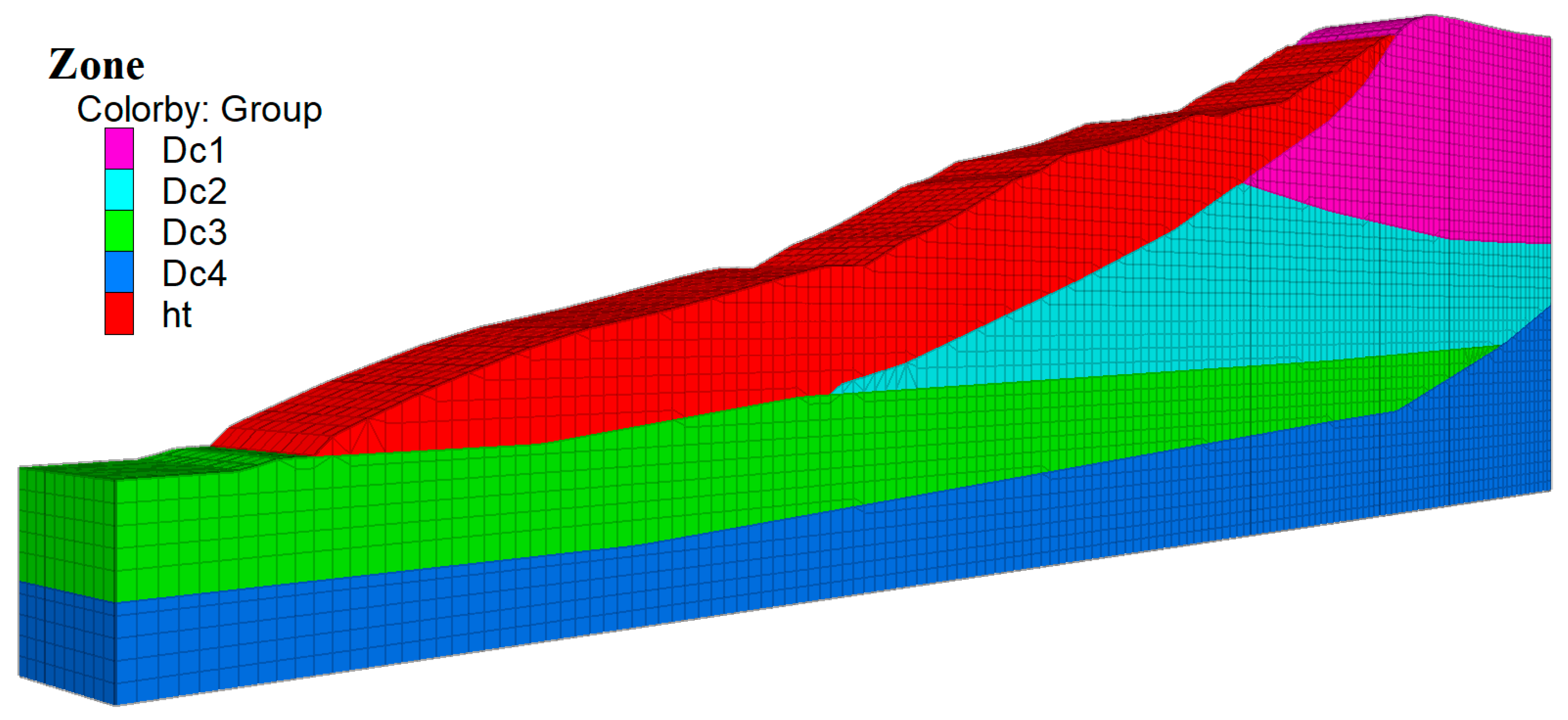
As shown in Figure 8, the model length and height are consistent with the profile, and the width is 10 m. The meshing process employs hexahedral and tetrahedral cells, resulting in a total of 49,371 nodes and 44,310 cells. The calculation assumes a fixed pile bottom, and the determined length of the pile is based on empirical evidence to ensure that the minipile can penetrate the clay rock layer by at least 3 m, which is temporarily set as 18 m in this study.

The soil parameters of the optimized calculation model were taken with reference to its surveyed stratigraphic parameters table, see Table 4. The structural unit parameters were taken according to

Table 7. Table of values of structural unit parameters.

Structure Type	Cross-Sectional Dimensions/m	Density g/cm3	Modulus of ElasticityE/GPa	Poisson’s Ratio μ	Polar Moment of Inertia/m4	Y-Axis Moment of Inertia/m4	Z-Axis Moment of Inertia/m4
Piles	φ0.15	2600	30	0.20	4.97 × 10−5	2.485 × 10−5	2.485 × 10−5
Connected beams	4.7 × 10.0 × 0.15	2600	30	0.20	——	——	——

.

The optimization procedure is calculated according to the preset relevant parameters, and its optimization process is shown in

Table 8. List of optimization results.

Number of Calculations	1	2	3	4	5
Pile length (m)	18	10	14	16	15
Safety factor	1.43	1.11	1.39	1.43	1.41

.

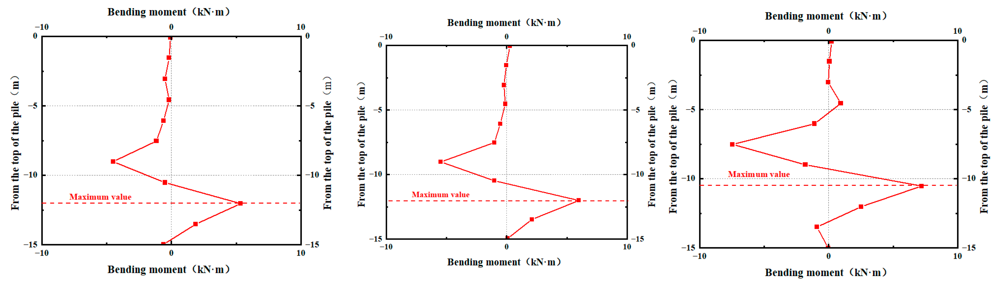
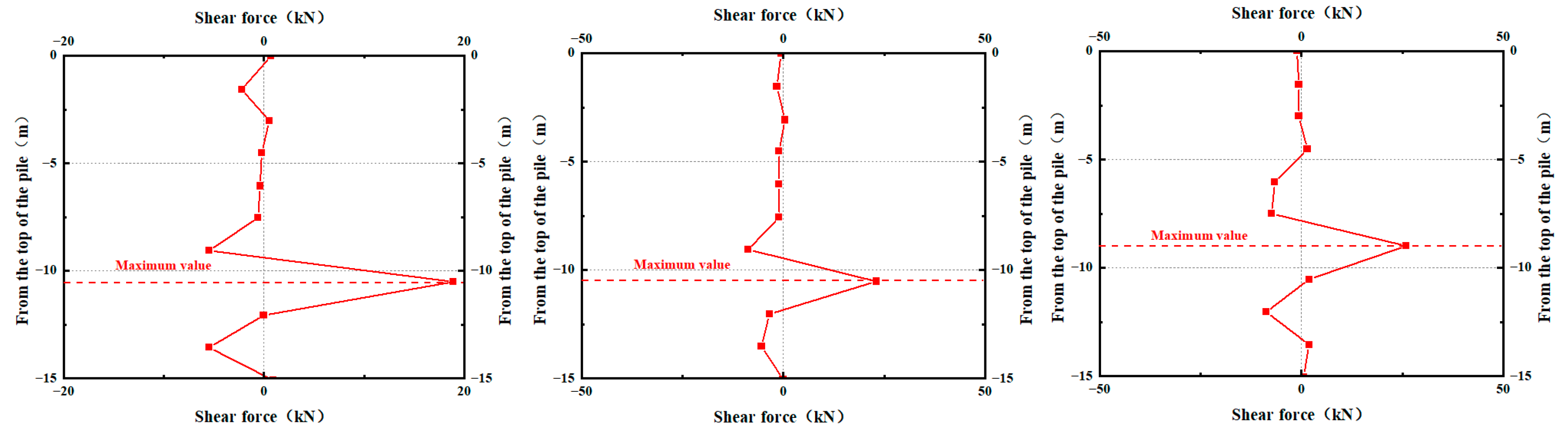
The pile length obtained from the optimization calculation is PL = 15 m. The internal forces of the minipile after the optimization calculation is completed are extracted, and the results of its bending moment and shear force calculation are presented in the following figures (Figure 9 and Figure 10). The numerical simulation results reveal that the rear row pile exhibits the highest bending moment, followed by the middle row pile, and finally, the front row pile displays the lowest bending moment. The maximum value of bending moment for all minipiles is 7.539 kN·m, and the maximum value of shear force is 26.47 kN, which is small compared with the results of theoretical calculations. As depicted in the figure, the numerical simulation results indicate that the rear row pile exhibits the highest bending moment, followed by the middle row pile and the front row pile with the lowest magnitude.

Overall, the optimized design has successfully achieved its intended objective, and through engineering practice, the calculation method and optimization approach outlined in the previous section have been demonstrated to be more dependable.

3. Results and Discussion

In this study, the design calculation method of a miniature pile and the optimization method of pile length are investigated comprehensively, and the algorithm of the miniature pile and pile length are optimized and improved by using numerical simulation modeling.

(1) Based on the load sharing theory and elastic foundation beam theory, the micropile calculation method of “whole to local split calculation” is summarized, the finite difference solution method for programming calculation is derived, the calculation formula is derived, and the calculation process is programmed.

(2) Based on the theoretical calculation results of the minipile, a mathematical model for pile length optimization was established, and numerical simulation using numerical simulation software was used for the optimization solution. The process is solved by programming numerical simulation fast modeling, automatic creation of optimization commands, and optimization result output analysis modules.

(3) According to the proposed minipile calculation method and optimization method, a specific analysis is carried out for an engineering example, and a series of studies, such as minipile design calculation and pile length optimization for this project, were completed. The engineering feasibility of the proposed minipile design calculation and optimization method has been demonstrated through practical application. The optimization process incorporates innovative ideas and implementation modules, which can serve as a reference for similar geotechnical engineering structure optimization problems.

(4) For this experiment, we have chosen to illustrate the problem with a general typical form of landslide, and the same applies to special cases, which we have considered in the modeling process. Moreover, this test is only applicable to the initial fast and flexible management of small landslides and is not applicable to large landslides, applying anti-slip piles and multi-row anti-slip pile management systems.

(5) In this study, the optimization calculation process, although the design variables as the geometric parameters of the structure body, but in the calculation process is the whole system (miniature piles and landslide body constitute the overall structure) to calculate the realization, to carry out the structural calculation is based on the relevant Chinese norms, fully taking into account the interaction between the piles and the landslide body influence. The safety and stability coefficients obtained from the calculations are not those of the piles themselves but those of the system environment.

(6) Due to the complexity of the miniature anti-slip pile governance system, the optimization model research body of literature is relatively small, the mainstream of the so-called optimization method for the list of individual methods and similar research results for comparison, the optimization method in this study is the optimization algorithm of the model, where the parameters and so on are derived from the calculation of the formula. Mainstream-related optimization results and costs can not be directly compared with the text of this research study’s results, so it needs to be followed by further research studies.