Sea Drift Trajectory Prediction Based on Quantum Convolutional Long Short-Term Memory Model

Abstract

This paper proposes a novel Sea Drift Trajectory Prediction method based on the Quantum Convolutional Long Short-Term Memory (QCNN-LSTM) model. Accurately predicting sea drift trajectories is a challenging task, as they are influenced by various complex factors, such as ocean currents, wind speed, and wave morphology. Therefore, in a complex marine environment, there is a need for more applicable and computationally advanced prediction methods. Our approach combines quantized convolutional neural networks with Long Short-Term Memory networks, utilizing two different input types of prediction to enhance the network’s applicability. By incorporating quantization techniques, we improve the computational power and accuracy of the trajectory prediction. We evaluate our method using sea drift datasets and AUV drift trajectory datasets, comparing it with other commonly used traditional methods. The experimental results demonstrate significant improvements in accuracy and robustness achieved by our proposed Quantum Convolutional Long Short-Term Memory model. Regardless of the input mode employed, the accuracy consistently surpasses 98%. In conclusion, our research provides a new approach for sea drift trajectory prediction, enhancing prediction accuracy and providing valuable insights for marine environmental management and related decision-making. Future research can further explore and optimize this model to have a greater impact on marine prediction and applications.

1. Introduction

Due to industrialization and population growth, global resources are becoming increasingly limited. As an essential resource for human survival in the 21st century, the ocean will significantly contribute to human and social progress [1]. Predicting the trajectory of ocean-floating objects is essential in various fields, including maritime safety, environmental protection, search and rescue operations, and maritime transportation. The ability to accurately predict the trajectory of floating objects such as oil spills, marine debris, and drifting vessels is crucial for a timely and effective response to emergencies and events at sea. For instance, in the case of an oil spill, accurate trajectory prediction can help determine the potential environmental impact of the spill and plan and implement effective response measures. In search and rescue operations, trajectory prediction can help identify the possible location of missing vessels or individuals and allocate search resources more efficiently.

The main problem in maritime trajectory prediction is forecasting the future trajectory of a vessel based on past observed vessel trajectory data. This is a challenging problem because the movement of vessels at sea is influenced by various factors, including ocean currents, wind speed, and the behavior patterns of the target vessel. Therefore, there is a need to develop an accurate method for predicting maritime vessel trajectories in order to provide reliable position and motion information at future time points.

This paper proposes a quantum convolutional Long-Short-Term Memory network (QCNN-LSTM). We quantized the CNN part to improve the computational power of the model and more effectively solve the gradient explosion problem. The connected LSTM part effectively enhances the model’s ability to predict sequence data and performs better spatiotemporal sequence prediction. The QCNN-LSTM method utilizes the efficient computation and strong fault tolerance advantages of QCNNs, which can better extract features and perform convolution operations on sequence data. Compared to traditional numerical methods, the QCNN-LSTM method can better capture the features of sequence data, improving the model’s prediction accuracy and effectiveness. Compared with other similar structured neural network models, the QCNN-LSTM method can significantly reduce the training and prediction time of the model, thereby improving its practicality and reliability.

The Section 1 of the paper introduces the background, problem statement, and significance of the research and outlines the research objectives and methods. The Section 2, related work, reviews and summarizes previous research findings and literature relevant to the research topic while also explaining the motivation for employing quantization techniques. The Section 3 presents the experimental part, providing a detailed description of the data used in the experiments and the evaluation criteria, and analyzing and discussing the results of the experiments. Finally, in Section 5, the paper is summarized and future work is discussed.

2. Related Work

The related work mainly introduces the results and literature on the prediction of sea-related trajectories, including traditional numerical models and some common neural network frameworks. The main findings, methods, and limitations of these studies are summarized. In view of these problems, the motivation for introducing quantization is proposed, and the advantages of quantization are explained.

2.1. Previous Research Results

Traditional numerical methods are one of the most important means for predicting drift trajectories. Zhang et al. used the Lagrangian model to predict the drift trajectories in the South China Sea [2]. Rabatel et al. studied the probabilistic prediction ability of the sea ice model NextSim used in the backtracking mode [3]. NeXtSIM is a continuous Lagrangian numerical model that uses viscoelastic rheology to simulate the response of ice to external forces. Chen et al. established a backtracking model for source analysis of marine floating objects [4]. Based on the Monte Carlo-based integrated trajectory model, the Leeway model, they proposed using virtual spatio-temporal drift trajectories for real-source analysis.

In standard ocean trajectory prediction, the prediction of oil spills [5,6,7,8] and algal migration and diffusion belong to the particle prediction problem [9,10]. In particle prediction, numerical methods and models are often used to simulate particle motion. However, due to the complexity and uncertainty of the marine environment, traditional numerical methods and models often face difficulties in accurately predicting the trajectory of floating objects.

Compared with traditional numerical methods, neural network models have stronger adaptability and generalization ability, higher prediction accuracy and computational efficiency, and require less data. These advantages make neural network models have a wide range of application prospects in drift trajectory prediction and have become a hot topic and trend in current research. The problem of predicting ocean drift trajectories is essentially a sequence prediction problem. Currently, popular prediction models mainly include recurrent neural networks (RNNs) [11,12], Long-Short-Term Memory Networks (LSTMs) [13,14,15,16], Transformers [17,18], and their variations.

The use of recurrent neural networks (RNN) for ship trajectory prediction is also an extensive research field. Samuele et al. extended the deep learning framework of ship trajectory prediction by exploring how the recurrent encoder-decoder neural network predicts through Bayesian modeling. Some researchers use the sequence-to-sequence model based on deep learning, combined with historical AIS observation data and additional input information (such as ship intention), to predict the ship trajectory [19] and use the sequence-to-sequence model and spatial grid for trajectory prediction [20].

Zhou et al. proposed an efficient transformer-based model called Informer for long sequence time-series forecasting (LSTF) that addresses the issues of quadratic time complexity [21]. Duong et al. used an improved transformer network, TrAISformer-A, to extract the correlation of AIS trajectories in the proposed enrichment space to predict the location of ships in the next few hours [22].

Convolutional neural networks (CNNs) can accurately extract features from multi-dimensional data and create highly accurate and robust models. However, they are not entirely suitable for learning time series and require additional processing. The Temporal Convolutional Network (TCN) uses one-dimensional convolutional layers to model sequences. These convolutional layers use a causal convolution operation that differs from traditional CNNs. TCN is a sequence modeling method based on convolutional neural networks (CNN) that can be used to process time series data. Compared with traditional recurrent neural networks (RNNs), TCNs can perform parallel computations, resulting in faster computation speeds. Additionally, TCN has good long-term dependency modeling capabilities [23,24,25]. There are clear differences in the use of TCN and CNN. TCN focuses on handling temporal data and modeling temporal relationships, making it suitable for temporal data analysis. It utilizes one-dimensional convolutional layers and temporal pooling layers to capture long-term dependencies and local features in temporal data. On the other hand, CNN typically consists of a series of two-dimensional convolutional layers and pooling layers, with relatively simpler connections between layers. CNN is more suitable for processing two-dimensional data and capturing spatial features, making it widely applicable in the field of computer vision. As the TCN network uses one-dimensional convolutional layers, it may be limited in capturing the features of time series data, such as periodic data with multiple time scales. Therefore, in some cases, TCN may not fully capture the characteristics of time series data.

Some scholars have proposed a CNN-LSTM hybrid framework for prediction [26,27,28]. The LSTM network is an excellent variant model of RNN that can better handle time series tasks and solve the gradient explosion problem in RNN networks. However, although the LSTM part of the model has been partially resolved in terms of gradient problems, it is still challenging to solve for many sequences. In addition, the LSTM model architecture is relatively complex and time-consuming to train. Due to these issues, quantum computing provides a new approach to solving problems that traditional computers cannot handle, as it offers a different computing environment [29,30]. In particular, superposition and entanglement, which are not initializable in classical computing environments, can achieve robust performance by utilizing the parallelism between quantum bits. Common quantum architectures proposed so far include Quantum Neural Networks (QNN) [31], Quantum Convolutional Neural Networks (QCNN) [32], and Quantum Long Short-Term Memory Networks (QLSTM) [33].

2.2. Motivation of Quantized Convolutional Neural Networks

When quantum neural networks are trained on large data sets, the problem of the ‘barren plateau’ (exponential vanishing gradient) will occur. However, researchers have shown that the landscape of QCNN models does not affect this problem when training on large data sets. Therefore, the QCNN architecture can be trained under random initialization of parameters. The QCNN-LSTM framework used in this paper effectively avoids the gradient explosion and gradient disappearance problems of common recurrent network models.

The QCNN part uses qubits for quantum computation and represents a variety of possible combinations of 1 and 0, connecting them to provide more processing power than the same number of binary files. By binarizing the parameters and weights in the network, the quantum neural network can reduce the memory occupied by the training while ensuring the training accuracy. By introducing the superposition idea of quantum states into the traditional feed-forward neural network, the activation function of the hidden layer of the neural network is superimposed by multiple S-shaped functions. An S-shaped function can only represent two orders of magnitude and states, and the linearly superposed sigmoid function has different quantum intervals between adjacent functions. The uncertainty of the input data of the training sample can be quantified by the training of the quantum interval because the hidden neural unit can represent more amplitude and state. By using the multi-layer activation function, different data are mapped to different amplitudes, which increases the fuzziness of the network and improves the accuracy and certainty of network pattern recognition.

In the model input part of the framework, quantum-dense coding converts data into qubits. Quantum entanglement enables one qubit to transmit multiple classical qubits, thus significantly expanding the channel capacity. A qubit contains two orthogonal (|0⟩ and |1⟩ or linear combination) states of a two-state system. If the auxiliary entanglement is a Bell state, then two classical pieces of information can be transmitted while transmitting a qubit; the entanglement-assisted classical channel capacity is twice the original.

3. Methods

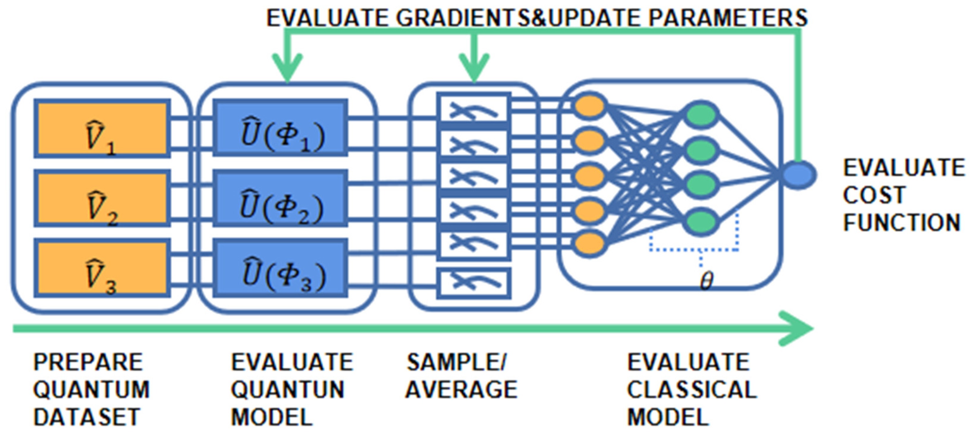
This paper uses the quantum model architecture in series with TensorFlow’s LSTM in the QCNN section. The CNN, LSTM, and quantum models are all built using Tensorflow and Tensorflow quantum in Python in the model training submodule. TensorFlow Quantum (TFQ) is a framework that integrates Cirq with TensorFlow. TensorFlow is an upper-layer framework for wrapping machine learning or deep learning algorithms. Cirq is closer to quantum computing device operation, including a variety of common logic gates, circuit design, and support for different structures of quantum devices (Google’s Xmon quantum device is mesh qubits). In essence, the TFQ model aims to embed quantum circuits into ordinary deep learning models and let quantum circuits encode the information of classical deep learning; Figure 1 is a high-level abstract overview of the computational steps involved in the end-to-end pipeline [34] and includes a hybrid quantum-classical discriminant model for reasoning and training quantum data in TFQ.

As shown in Figure 1, information in the classical world can be encoded by formulating some quantum circuit operations and “disentangling” the input qubits [35]. This section will first introduce the data transformation used for the quantum model, and then describe how the transformed quantum data is fed into a quantum-inspired neural network. Subsequently, the overall construction of the model will be presented, followed by a discussion of the advantages of our model over traditional numerical models and conventional neural networks.

3.1. Software Setup

The model development incorporates the workflow pipeline and checkpoint design patterns to ensure model reproducibility and flexibility. The workflow pipeline design pattern ensures model reproducibility, while the checkpoint design pattern reduces overfitting by saving the model instance with the lowest validation loss. The preprocessing layer removes low-correlation features. For short-term memory-based prediction models, the StatsModel API is used for exponential smoothing to maintain stability in the training data. In models built on quantum architecture, the dense angle encoding proposed by LaRose and Coyle is applied with Cirq [36].

Python’s TensorFlow and TensorFlow Quantum are used to build classical and quantum models. The checkpoint design pattern is used to prioritize fault tolerance and flexibility for all models. After each training epoch, the validation loss is measured. If the validation loss is lower than the previous epoch, a snapshot of the model state is saved for future training recovery. The patience time, which is the time to interrupt the training process if the validation loss does not improve, is set to 100 epochs. This ensures that the algorithm has enough time to avoid potential local minima during optimization. The data is continuously validated to maintain the consistent dimensionality of the dataset and the separation between training and testing data.

Finally, the validation submodule initializes with the saved model and obtains the key metrics described in the methodology section. These metrics, along with the generated predictions, are saved in a subfolder.

3.2. The Quantization of Data

In the QCNN part of the model, the input data needs to be further transformed to encode it into a quantum circuit that can be measured to obtain the desired value [36]. Encoding can be referred to as “loading” data points from memory into the quantum state, and encoding functions do this loading from the dataset into the bit quantum state. First, a single-qubit rotation gate can perform phase rotation:

$$R(\theta )=\left[\begin{array}{cc}\cos \theta & -\sin \theta \\ \sin \theta & \cos \theta \end{array}\right],$$

(1)

Suppose the quantum state:

$$|\mathrm{\varnothing }⟩=\left[\cos {\theta }_0\sin {\theta }_0\right],$$

(2)

When a single-qubit rotation gate $R\left(\theta \right)$ is applied to the state $|\mathrm{\varnothing }⟩$:

$$R\left(\theta \right)|\mathrm{\varnothing }⟩=\left[\cos {\theta }_0+\theta \sin {\theta }_0+\theta \right],$$

(3)

The method used in this paper is to convert each feature $x\in X$ into a quantum state, which is then added to the quantum circuit as an input. A set of input features $x$ is encoded as an n-quit quantum state $D_n$, and the feature vector $x={\left[x_1,\cdots ,x_N\right]}^T\in X^N$ can be encoded into a quantum circuit:

$$|x⟩={⨂}_{i=1}^N \cos \left(x_i\right)|0⟩+\sin \left(x_i\right),$$

(4)

The ready-state unitary operator is set to $S_{x_j}={⨂}_{i=1}^N U_i$ and is obtained by the following equation:

$$U_i=\left[\begin{array}{cc}\cos (x_j^{\left(i\right)})& -\sin (x_j^{\left(i\right)})\\ \sin (x_j^{\left(i\right)})& \cos (x_j^{\left(i\right)})\end{array}\right],$$

(5)

3.3. The Input of Model

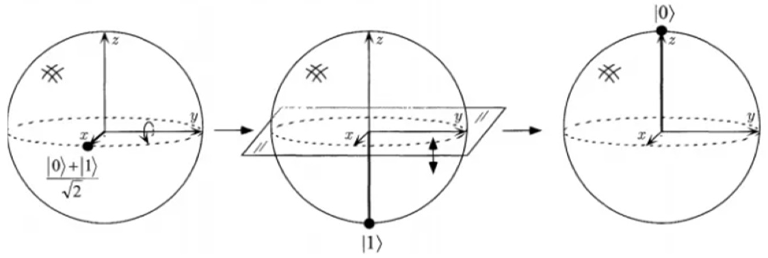
In this study, we conducted comparative experiments between the CNN, CNN-LSTM, and QCNN models. The input of the QCNN and QCNN-LSTM models needs to quantize the data, which means rotating the quantum state on the Bloch sphere [37] around the X, Y, and Z axes by angles, so it can bring about a change in the probability amplitude. However, only phase changes and the use of these three operations together can make the quantum state move freely on the whole Bloch sphere [38] (Figure 2).

As mentioned in the introduction, the CNN model cannot be directly used for time series prediction, so we improved several models for this purpose. For drift trajectory data, sometimes the data is periodic, while other times it is discrete and non-periodic. To enhance the models’ versatility, they were designed to accept two types of inputs: discrete data input (without providing short-term memory to the model) and periodic data input (with input length corresponding to the autocorrelation period).

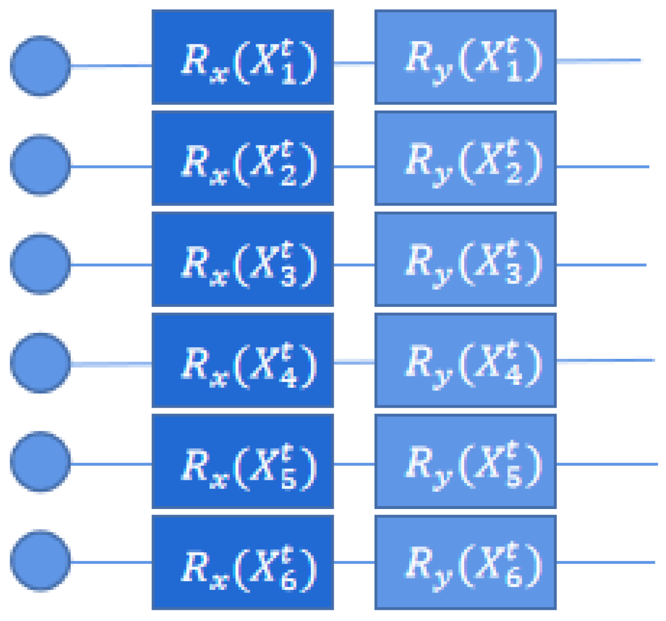
For the first type of input, all input data points are considered discrete, so accuracy can be achieved by simply fitting the regression to each data point, and the model’s historical input does not affect it; each row of data is independent of historical data. Figure 3 shows the QCNN model for discrete input data with quantum circuits encoding the data into dense-angle representation. Each quantum circuit accepts feature data and rotates the input quantum state along the X and Y axes. Here, $X_1$ represents the first variable of the data, $X_2$ represents the second variable, and so on.

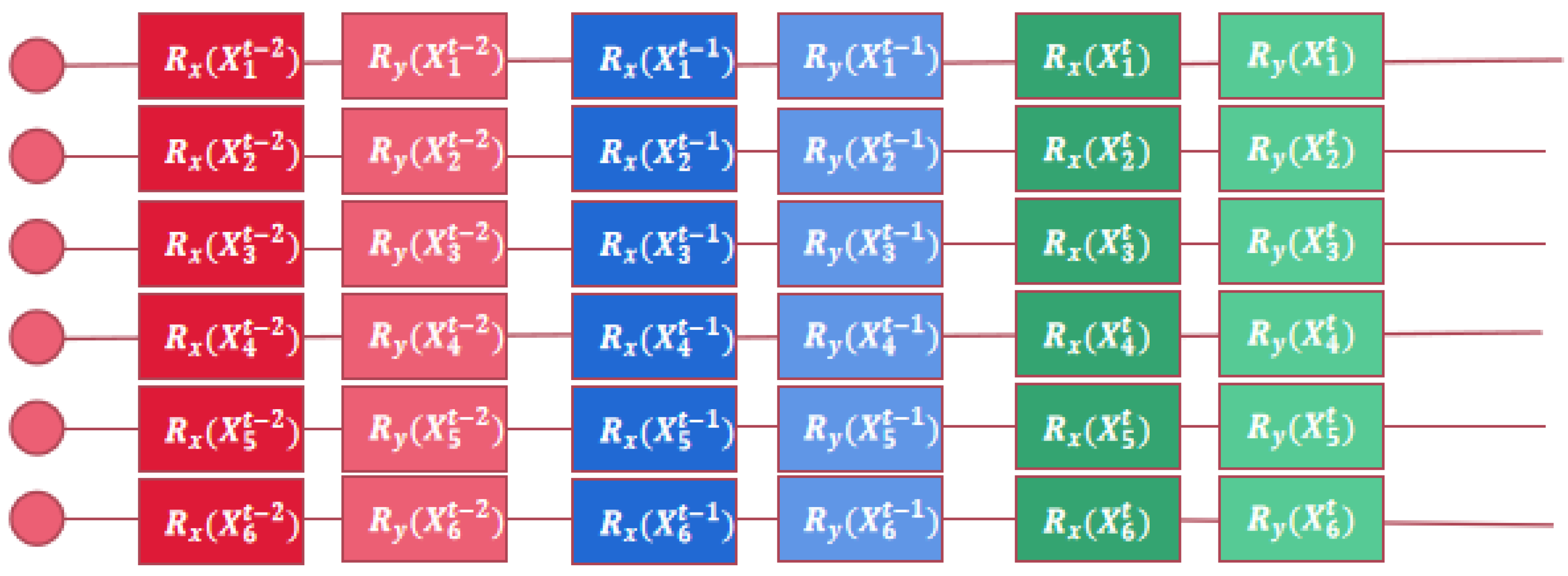
The second type of input that considers historical input data is the simulated “time window” input, which accepts input features of length n, where n is the observed autocorrelation period. Short-term memory is simulated for the model by providing input features of length n. The QCNN model with short-term memory and the QCNN-LSTM model needs historical data as input. We want the data set of each circuit to be stacked as a sequence as the input of the QCNN model. However, the input of each quantum circuit is always one quantum bit. In order to solve this problem, the input circuit will be connected in series with the time circuit as the historical data of the time circuit. The structure of the input quantum circuit is shown in Figure 4.

By testing the data set, it was found that the autocorrelation of the data set is set to 3 days, which is the best effect, and the sliding window with a length equal to the autocorrelation period is used to split the data set into small data subsets for input. If the autocorrelation period of the data is 3, then we only need to concatenate t with t − 2 and t − 1 like Figure 4.

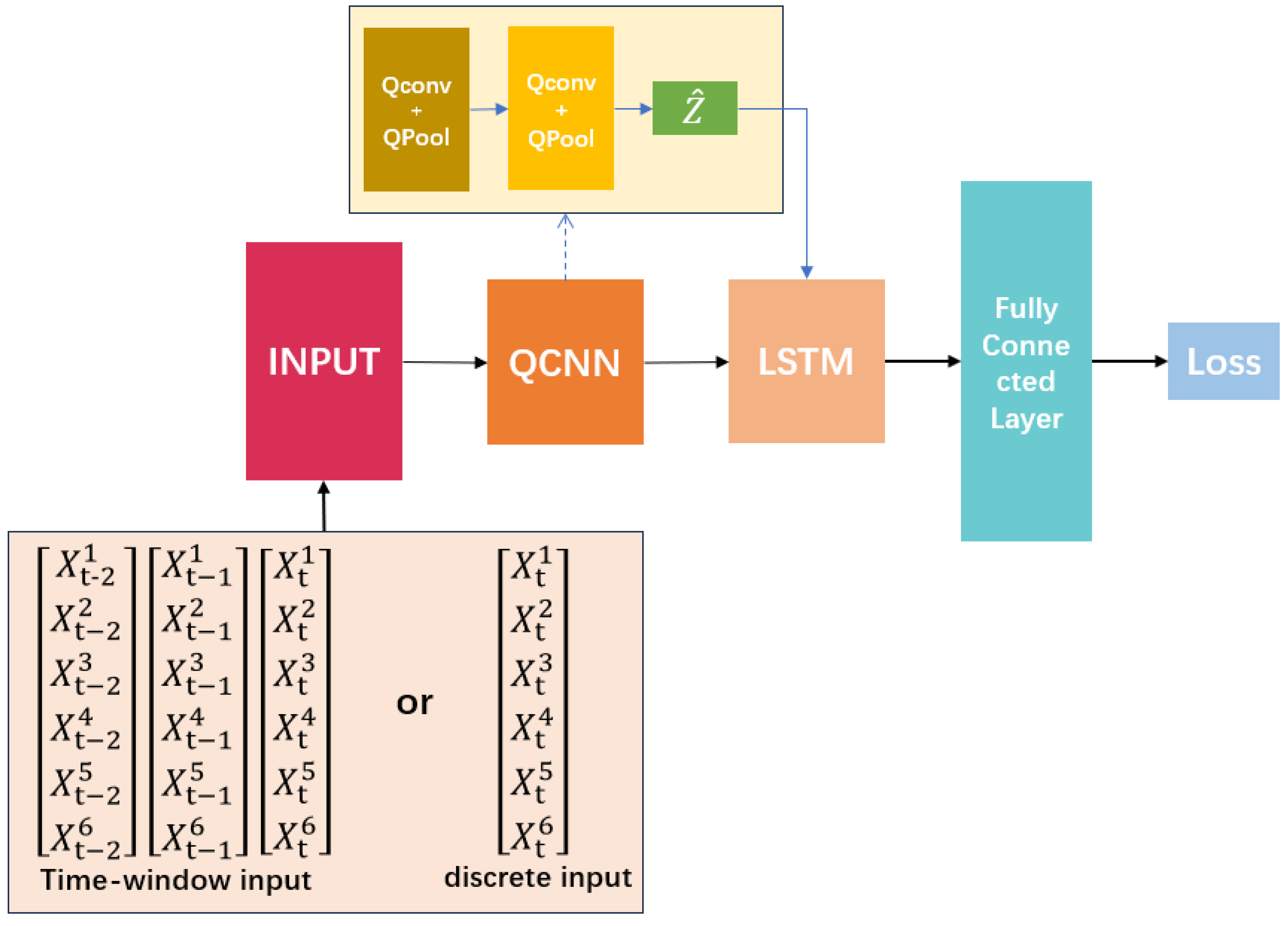
3.4. QCNN-LSTM Model Architecture

The QCNN-LSTM model requires three pairs of quantum convolutional and quantum pooling layers to accept quantum-encoded data, represented by a single quantum circuit composed of 6 qubits, with each qubit representing an input feature. A parameterized quantum circuit layer (PQC) is added after the QCNN layer to obtain the output as an MLP. The Z-axis transformation is used to measure the quantum state of the qubit.

A differential operator is used to explain how to measure the gradient of the quantum circuit. The differential operator serves as the quantum gradient descent function, which performs differentiation through forward and backward propagation of the quantum circuit. The Adam optimizer is used during the optimization process of the QCNN layer to estimate the parameters through backpropagation and minimize the mean squared error.

The convolutional part of the quantum convolutional layer uses the “LeakyReLU” activation function to evaluate the output from the convolutional operator, the bias term, and the feature map of the continuous layer. The following equation gives the evaluation of the output feature map of the convolutional layer:

$$x_j^l=lrelu\left(z_j^l\right)$$

(6)

$$z_j^l=\sum _i{x}_i^{l-1}\odot k_{ij}^l+b_j^l$$

(7)

The input of the convolutional filter is $x_i^{l-1}$, the output $x_t^l$, k is the convolution kernel, b is the paranoia term, and lrelu() stands for the “LeakyReLu” function. $\odot$ denotes the convolution operator and $z_j^l$ is the input of the LeakyReLu.

At this point, the qubits are folded into the bit state of the computer and passed to the LSTM framework in a one-to-one manner, as the data has already been flattened in the convolutional part. Finally, it is connected to a fully connected layer to fit and predict the transmitted data, and the output is the predicted value at that time. The difference between the predicted and actual values is calculated to obtain the error for evaluating the performance of the model framework.

Figure 5 illustrates the framework of the QCNN-LSTM model. The model can accept either discrete data or periodic time-window data as inputs, and different data types will be processed differently. The inputs $X^1$ through $X^n$ represent the n feature variables of the dataset. In the context of drift trajectory prediction, these variables include the latitude, longitude, speed, direction, temperature, and other environmental factors of the drifting object. In the input section of the framework, quantum-dense coding transforms data into quantum bits. The entanglement property of quantum bits allows one qubit to transmit multiple classical bits, greatly expanding the channel capacity [39]. Each quantum bit contains two orthogonal states ($\left|0⟩\right.$ and $\left|1⟩\right.$, i.e., a linear combination). If the auxiliary entanglement is in a Bell state, transmitting 1 quantum bit can transmit 2 classical bits of information. Therefore, the entanglement-assisted classical channel capacity is doubled.

After the data is input into the framework, spatial features are extracted in the QCNN section, and temporal features are extracted in the LSTM section, giving the model an advantage in spatiotemporal prediction. QCNN is used as the encoder in the encoder-decoder structure. Although QCNN does not directly support sequential input, modifying the convolution layers to be one-dimensional allows it to read sequential input and automatically learn salient features. The LSTM decoder can interpret this data. Matrix multiplication in LSTM is converted into a convolution operation and concatenated with LSTM after one-dimensional convolution. Finally, the fully connected layer uses a deep neural network with a single hidden layer as the output layer of the QCNN-LSTM network model to fit and predict the data, and the output is the predicted value at time t. This retains the high computational performance of the QCNN model while incorporating the LSTM model, giving the framework higher sequential prediction capability.

4. Experiment

In our experiment, we trained our model using ocean current data, and we divided the dataset into training, testing, and validation sets. To demonstrate the generalization of the model, we fine-tuned it and made predictions on underwater vehicle drift trajectory data. We compared the performance of our QCNN-LSTM model with other selected models. This paper begins by introducing the selection and processing of the data, followed by an explanation of the evaluation metrics used in the experiment. Lastly, we discuss the reasons behind choosing these models as our comparative models. In the experiment, we configured several hyperparameters. The learning_rate was set to 0.001 to ensure the stability of the model during training and avoid instability caused by overly large parameter updates. The batch_size was set to 1 to implement the training method of stochastic gradient descent, where only a single sample is used for parameter updates at each iteration. The number of epochs was set to 100 to ensure sufficient iterations over the dataset during training, allowing the model to better learn the features of the data and achieve improved performance.

4.1. Data Sets

In the prediction of the trajectory of ocean floating objects, the trajectory of ocean currents is an important component of the prediction, and for some small and low-wind resistance objects, we approximate their drift trajectory as the trajectory of ocean currents in the current sea area when the uncertain factors of the objects themselves are unknown. Therefore, we decided to first use a model to predict the trajectory of ocean currents in a specific sea area. In order to demonstrate the model’s generalization ability, we fine-tuned the model to predict the drift trajectories of relevant AUVs. The ocean current data is from the ship-mounted ADCP dataset of scientific investigation over the South China Sea [40], while the AUV data is from the BCO-DMO website [41].

For the ocean current data, since the daily variations are small and the number of data points per day is inconsistent in the dataset, we applied the median aggregation method during data preprocessing to merge multiple data points from the same day into a single data point. Using the median allows us to capture the central position of the ocean current trajectories for a given day, minimizing the impact of outliers. This approach helps eliminate the interference of anomalous ocean current data, provides a more accurate depiction of the central position and primary flow direction of the currents, and facilitates the identification of underlying periodic patterns in the data.

The ocean current data consists of ten features: date, time, longitude, latitude, observation layer, east component, north component, flow speed, flow direction, and probe temperature. We conducted a correlation analysis between each column of the dataset and the target variable to select the most relevant features. The columns were sorted in descending order based on the absolute values of their correlation coefficients. We then chose the top six variables with the highest correlation and used them for training.

During data preprocessing, we employed linear interpolation to fill in missing values, removed outliers, and standardized the data by subtracting the mean and dividing by the standard deviation to achieve a mean of 0 and a standard deviation of 1. We also examined the periodicity of the data and tested for autocorrelation periods. A similar approach was applied to the processing of AUV data.

4.2. Evaluation Parameters of the Test

To assess the performance of the prediction model, objective metric data was utilized. The dataset was divided into training, validation, and test sets in an 8:1:1 ratio. Performance metrics, including mean percentage error (MAPE), accuracy, root mean square error (RMSE), and mean error (MAE), were employed. The validation set was used to evaluate the in-model prediction performance, while the training set was utilized to measure the out-of-model prediction performance. The working rates of quantum CNNS and existing CNNS were determined by recording the time required to achieve the minimum verification loss. Due to the increased conversion between quantum architectures caused by quantum information coding, the original RMSE and MAE values underwent changes in scale. Therefore, the RMSE% and MAE% error indicators were adopted to assess the accuracy between the two architectures. Here, $e_t, f_t, \mathrm{a}\mathrm{n}\mathrm{d} d_t$ are the error, predicted value, and expected value at time t.

$$e_t=f_t-d_t,$$

(8)

$$MAPE=\frac{1}{n}\sum \frac{\left|e_t\right|}{d_t},$$

(9)

$$Accuracy\%=100(1-MAPE),$$

(10)

$$MAE\%=\frac{\sum \left|e_t\right|}{\sum d_t},$$

(11)

$$RMSE\%=\frac{\sqrt{\frac{1}{n}\sum e_t^2}}{\frac{\sum d_t}{n}},$$

(12)

4.3. Choosing and Justifying Comparative Experimental Models

We attempted to use traditional dynamic numerical methods for drift prediction but found that they were not applicable to the dataset we had obtained. It is difficult to obtain accurate initial conditions for drift trajectory prediction in the ocean, and the accuracy of physical models established with current meteorological data and environmental factors is very low. Even if a specific ocean environment is simulated for prediction, the choice of parameters is a major issue, and the model may not have good adaptability to the drift trajectories of floating objects in other environments. Our goal is to create a low-cost, simple, and highly adaptable model that can be applied to a variety of ocean climates and floating objects. Therefore, we chose to use neural networks for prediction.

The neural networks selected for comparison with models are CNN, CNN-LSTM, and QCNN models. The decision to improve simple CNN and CNN-LSTM networks, rather than choosing more complex neural networks, is often based on a balance between model performance and computational complexity. Although more complex neural networks may achieve higher accuracy, they typically require more computational resources and may be more difficult to train and interpret. On the other hand, these two networks are relatively simple and mature architectures that have been proven effective in a wide range of applications. Adapting these two networks to the quantum model may be an effective strategy to achieve high accuracy while minimizing computational complexity and training time. They also allow us to leverage the advantages of these two architectures and create a highly suitable model for a wide range of applications.

The QCNN model provides us with a neural network for quantum-inspired improvement, but the QCNN model is good at capturing spatial features, while LSTM is very suitable for processing time-series data and handling long-term dependencies. By combining these two architectures, we can create a model that can capture both spatial and temporal features, making it highly suitable for a wide range of applications.

4.4. Experimental Analysis

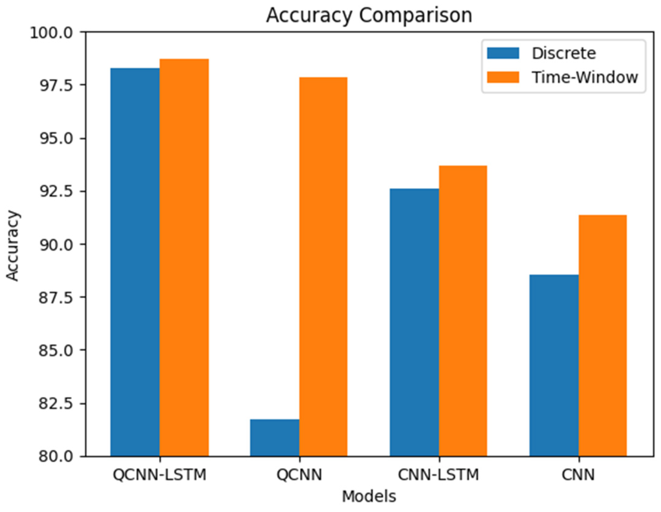
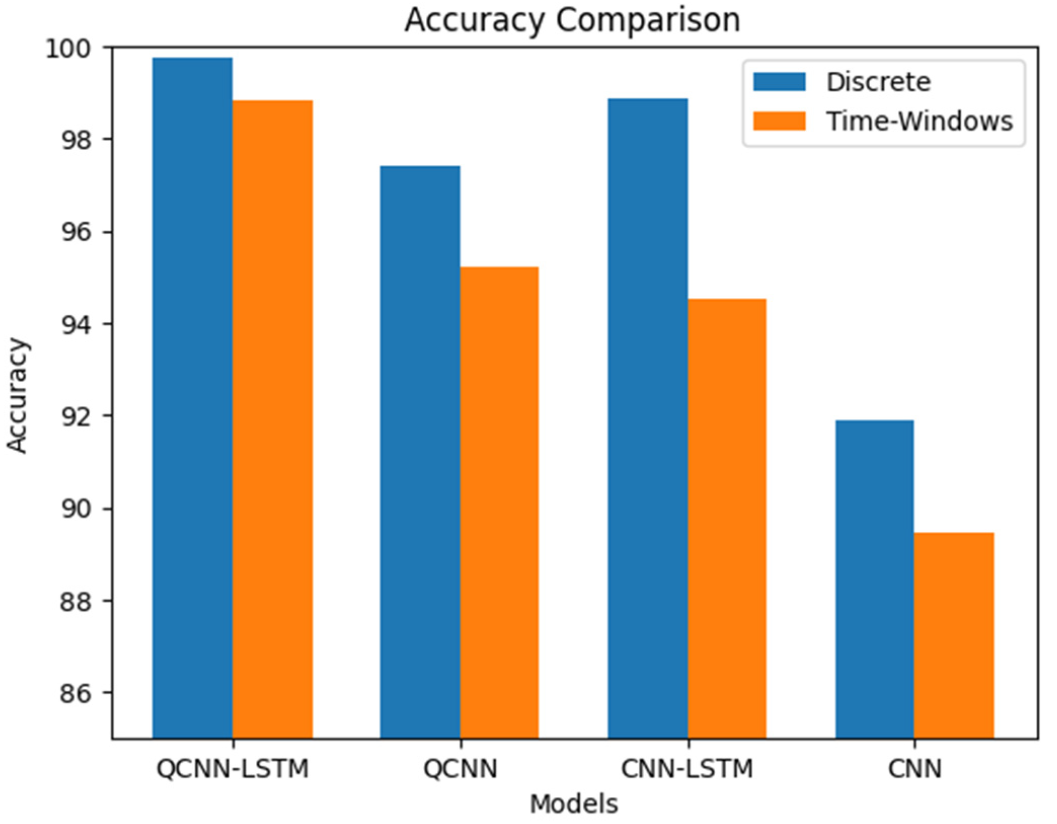
The experimental results show that the improved CNN network can also achieve good prediction results for trajectory data, a type of time series data. However, our QCNN-LSTM model achieved the highest accuracy, with the QCNN model slightly outperforming the CNN-LSTM model by about 5%. As the quantum encoding output of the quantum model changes the scale of the output data, RMSE and MAE are not compared. Instead, RMSE% and MAE% are used to make the results more accurate.

Table 1. The results of running the four models.

MAPE	ACCURACY%	RMSE%	MAE%	TYPE
0.017176	98.282445	1.938723	1.728665	qcnn_lstm_discrete
0.013070	98.693044	1.517768	1.316671	qcnn_lstm_time-window
0.183006	81.699374	16.895380	16.192391	qcnn_discrete
0.021535	97.846532	9.983868	6.016774	qcnn_time-window
0.074098	92.590254	10.180566	7.332311	cnn_lstm_discrete
0.063243	93.675709	7.229650	6.256379	cnn_lstm_time-window
0.114596	88.540435	11.830668	11.414632	cnn_discrete
0.086501	91.349870	9.383199	8.602466	cnn_time-window

compares the results of the validation set, comparing the QCNN-LSTM model with the CNN-LSTM model and the CNN model with the QCNN model, validating that the addition of the quantum part improves model accuracy by an average of about 3%. Comparing the CNN-LSTM model with the CNN model validates that the addition of the LSTM part improves model accuracy by an average of about 6%. The QCNN-LSTM model achieves the best accuracy and RMSE%MAE% regardless of whether historical or discrete data is used as input, with accuracy above 98%. The QCNN-LSTM model with simulated time window input can achieve a maximum accuracy of 98.69%. The QCNN-LSTM model with discrete input is slightly lower but still has an accuracy of over 98%.

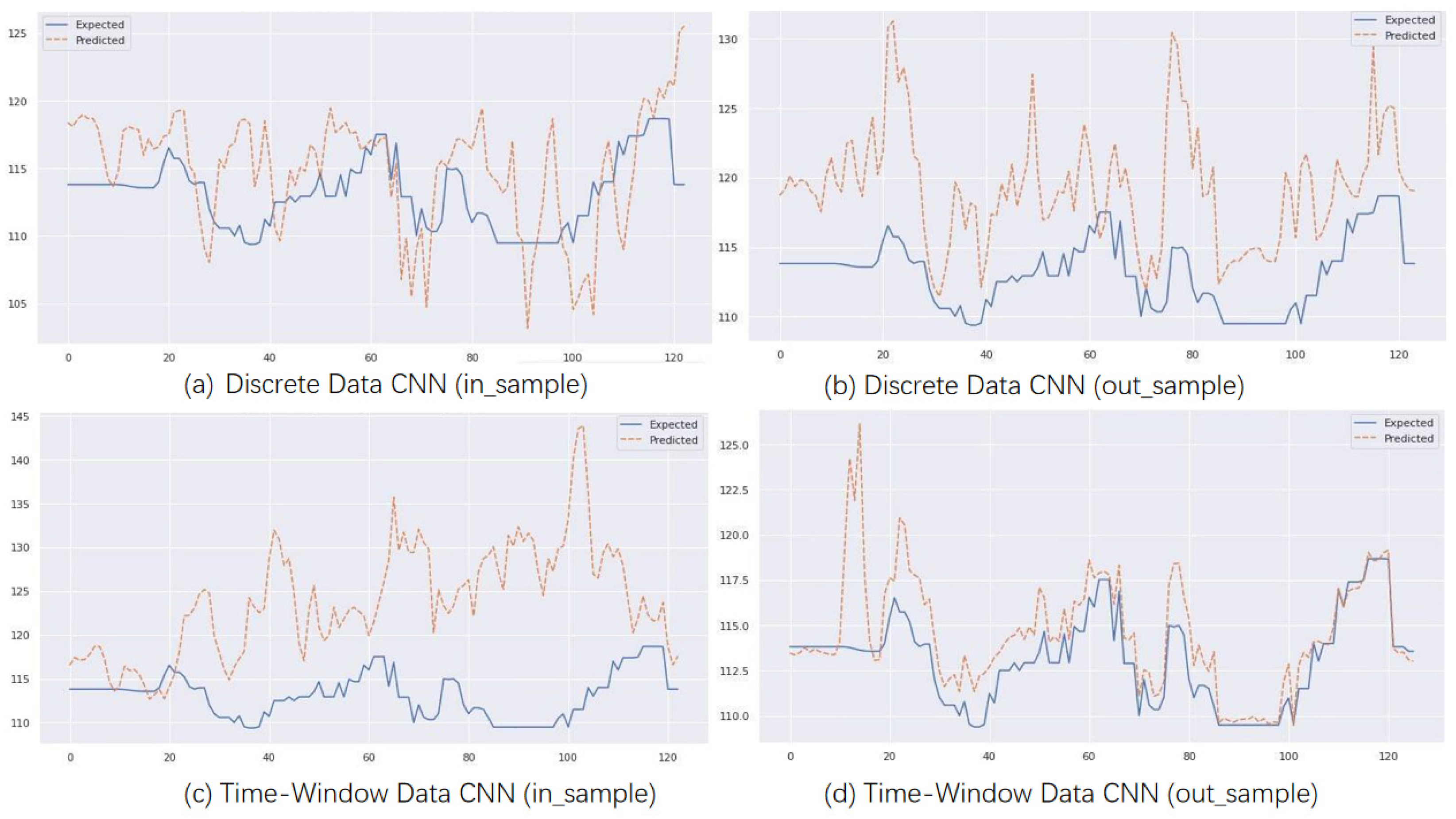
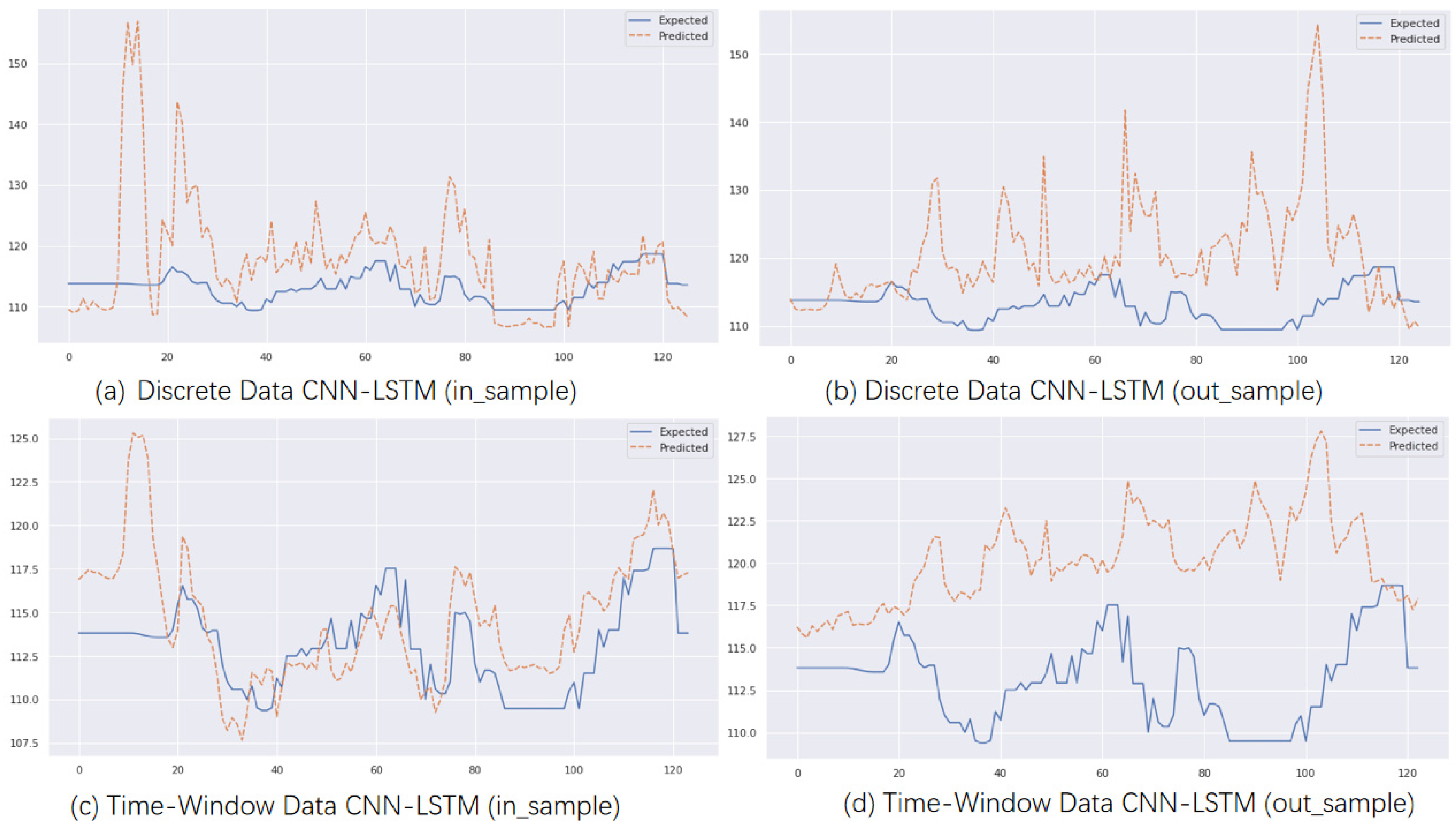
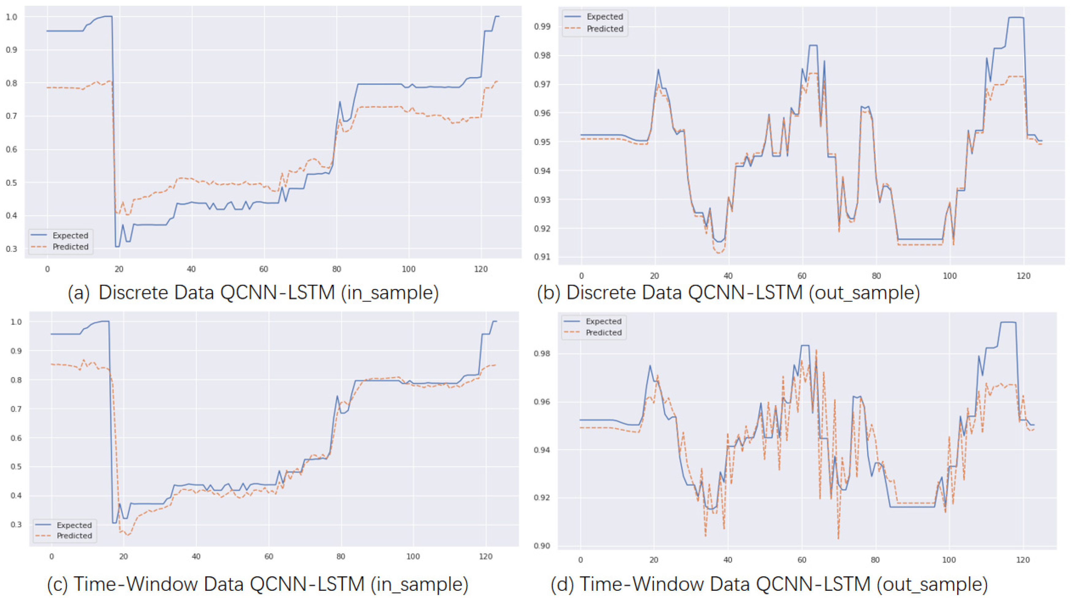
Figure 6 shows the prediction performance of the CNN model, while Figure 7 shows the prediction performance of the CNN-LSTM model. The CNN-LSTM model appears to be more stable than the CNN model, but surprisingly, the CNN model performs better for out-of-sample predictions with time window input. The latter half of the model closely matches the original data.

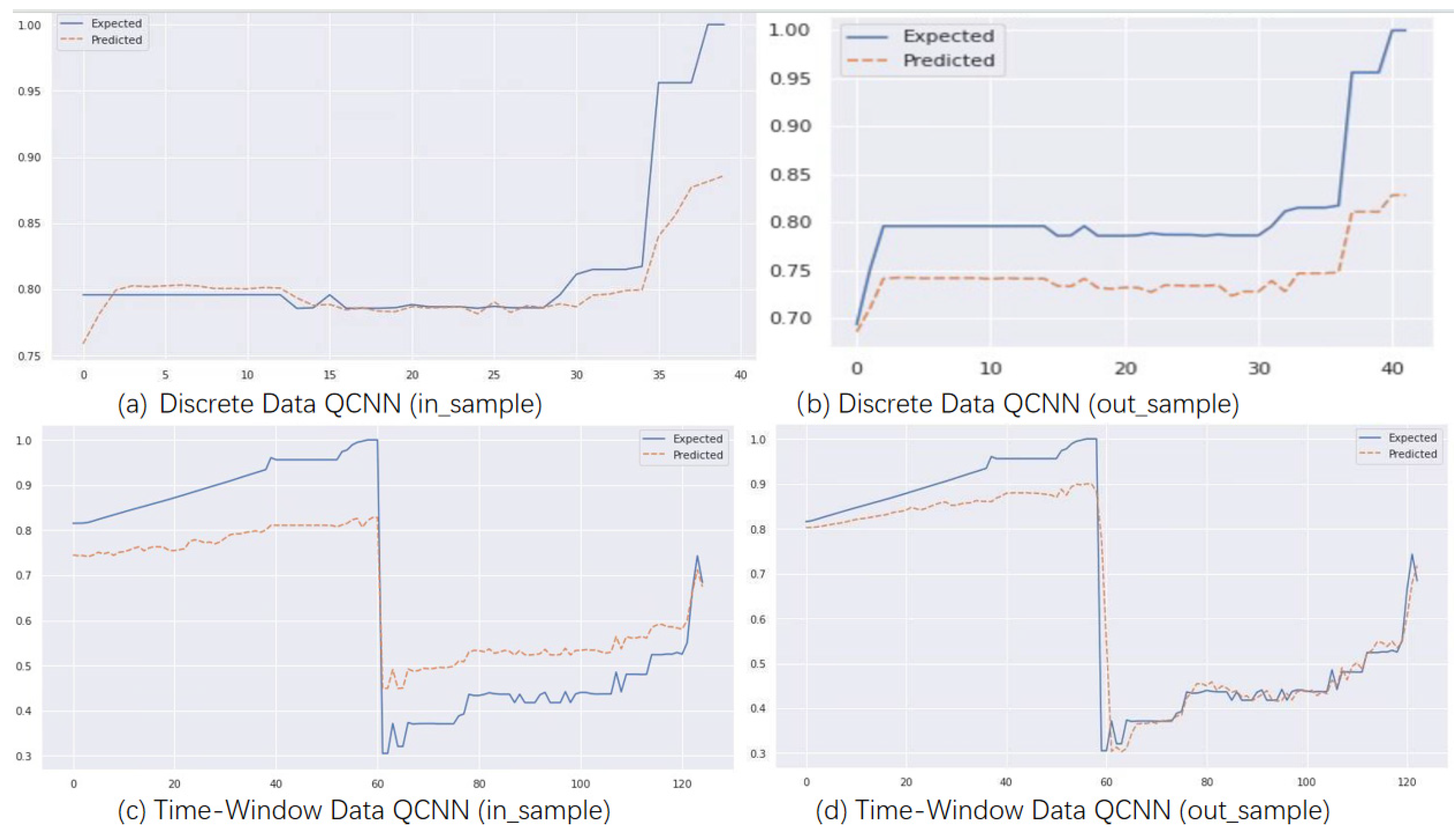
Combining Figure 6, Figure 7, Figure 8 and Figure 9 shows that the quantum model in the figure can more accurately fit the trend of the original data, and the QCNN and QCNN-LSTM models can more accurately track the trend of longitude and latitude drift during the prediction process compared with the CNN and CNN-LSTM models. As indicated in the third section of the QCNN-LSTM model, quantum bits can represent multiple possible combinations of 1 and 0 simultaneously, while regular computer bits can only have two states of 0 or 1. A quantum computer with multiple superimposed quantum bits can cancel out a large number of possible calculation results simultaneously.

All the models were designed with a single output during development; different predictions are required for predicting longitude and latitude. To make the visualization of results representative, the CNN model and CNN-LSTM predict latitude, QCNN predicts longitude, and the QCNN-LSTM model uses longitude for in-sample prediction and latitude for out-of-sample prediction. In terms of running time efficiency, the CNN model architecture runs faster than the QCNN model architecture. Without adding quantum structure, the average training time of the model is around 7 min, while the runtime of the QCNN model is about 12 min. The QCNN-LSTM model completes the run in about 17 min.

During the experiment, we identified the periodicity of ocean current data and determined its autocorrelation period to be 3 days during data preprocessing. On the other hand, AUV data is discrete and has no periodicity.

Therefore, selecting different input methods for different data types can improve prediction accuracy, as shown in Figure 10 for periodic ocean current data and Figure 11 for discrete AUV trajectory data. These figures demonstrate that our improved models can effectively capture the characteristics of different data types and make accurate predictions.

Furthermore, we can see from the figures that, even after fine-tuning our improved models, high accuracy can still be achieved when predicting the AUV dataset. However, our proposed QCNN-LSTM model still achieves the highest accuracy, indicating that our model has strong generalization ability and can maintain high prediction performance with less computation under limited conditions.

5. Conclusions and Future Work

The QCNN-LSTM model has the ability to effectively estimate multiple variables to some extent, even when these variables are not completely coupled or independent. However, the QCNN-LSTM model is sensitive to the degree of correlation between variables and the characteristics of the data. If there is a strong correlation or coupling between variables, the model can provide more accurate estimates. Conversely, if the correlation between variables is weak or if there are non-linear relationships, the model may face challenges and require more training and adjustments to capture their complex relationships.

Furthermore, the design of the model and the quality of training also impact the estimation capability. Appropriate model architecture, proper selection of hyperparameters, and sufficient training data with effective training strategies are all important factors to ensure that the model can effectively estimate multiple variables.

In summary, we employed common evaluation metrics for ocean trajectory prediction (or time series data) in our experiments to validate the proposed method. Based on the tabular data and graphical information, it can be concluded that our QCNN-LSTM model achieved an accuracy of over 98%, outperforming the comparison models for both discrete and periodically autocorrelated data. Furthermore, this high accuracy demonstrated stability across multiple subsequent experiments, and the model also achieved the lowest RMSE% and MAE%. These findings highlight the superiority of the model we utilized.

However, this approach also has certain limitations. For handling long sequence data, I would recommend using the Transformer model. Long sequence data often involves longer dependencies, and the Transformer model, with its self-attention mechanism, effectively captures global dependencies and excels at modeling long-range dependencies. In contrast, the QCNN-LSTM model may face challenges with long-term memory retention. Additionally, when dealing with large datasets, the QCNN-LSTM model may have limitations, as quantizing the data and inputting it into QCNN-LSTM requires higher hardware requirements and computational power, potentially necessitating the use of quantum computers. The choice of model should consider specific task requirements, dataset size, and characteristics. In some cases, if the dataset is small or exhibits clear local patterns, the QCNN-LSTM model may still be a reasonable choice.

This article presents the application of quantization in time-series data prediction, where we propose and develop the QCNN-LSTM model for sequence data prediction. Introducing quantization in the convolutional part of the model has improved computational power and avoids the problem of gradient explosion. Leveraging the unique properties of quantum bits to represent multiple possibilities simultaneously can lead to more complex calculations and higher accuracy. We have also improved the input method of the model to allow for different input types, making the model more targeted and improving its generalization ability.

As quantum hardware continues to improve, quantum models can be further optimized and scaled up to solve larger and more complex problems. Combining classical and quantum models can leverage both strengths to achieve higher accuracy and computational efficiency. Since the LSTM model is a popular time series prediction model, future work will also consider directly developing quantum LSTM models for multivariate regression. Furthermore, we plan to develop end-to-end prediction software that can efficiently perform predictions on different types of data. Regarding the adjustments and optimizations of the model structure, we will consider incorporating other types of neural network layers, such as the Attention Mechanism, to enhance the model’s expressive power and generalization ability. LSTM models may encounter the issue of long-term dependencies when dealing with long sequences. Therefore, we will also explore the combination of other recurrent neural network structures with quantum theory, such as the Gated Recurrent Unit (GRU) or Transformer, to improve the model’s ability to capture long-term dependencies.

References

- Wu, Y.; Zhao, Y.; Lang, S.; Wang, C. Development of autonomous underwater vehicles technology. Strateg. Study Chin. Acad. Eng. 2020, 22, 26–31. [Google Scholar] [CrossRef]
- Zhang, X.; Cheng, L.; Zhang, F.; Wu, J.; Li, S.; Liu, J.; Chu, S.; Xia, N.; Min, K.; Zuo, X.; et al. Evaluation of multi-source forcing datasets for drift trajectory prediction using Lagrangian models in the South China Sea. Appl. Ocean. Res. 2020, 104, 102395. [Google Scholar] [CrossRef]
- Rabatel, M.; Rampal, P.; Carrassi, A.; Bertino, L.; Jones, C.K.R.T. Impact of rheology on probabilistic forecasts of sea ice trajectories: Application for search and rescue operations in the Arctic. Cryosphere 2018, 12, 935–953. [Google Scholar] [CrossRef]
- Chen, Y.; Zhu, S.; Zhang, W.; Zhu, Z.; Bao, M. The model of tracing drift targets and its application in the South China Sea. Acta Oceanol. Sin. 2022, 41, 109–118. [Google Scholar] [CrossRef]
- Beegle-Krause, C.J.; Nordam, T.; Reed, M.; Daae, R.L. State-of-the-Art Oil Spill Trajectory Prediction in Ice Infested Waters: A Journey from High Resolution Arctic-Wide Satellite Data to Advanced Oil Spill Trajectory Modeling-What You Need to Know. Int. Oil Spill Conf. Proc. 2017, 2017, 1507–1522. [Google Scholar] [CrossRef]
- Xiong, D.; Zhang, X.; Lamine, S.; Liao, G. Numerical Simulation of the Trajectory and Fate of Spilled Oil at Sea. In Proceedings of the 2010 4th International Conference on Bioinformatics and Biomedical Engineering, Chengdu, China, 18–20 June 2010; pp. 1–4. [Google Scholar]
- García-Martínez, R.; Flores-Tovar, H. Computer Modeling of Oil Spill Trajectories With a High Accuracy Method. Spill Sci. Technol. Bull. 1999, 5, 323–330. [Google Scholar] [CrossRef]
- Zhu, K.; Mu, L.; Xia, X. An ensemble trajectory prediction model for maritime search and rescue and oil spill based on sub-grid velocity model. Ocean. Eng. 2021, 236, 109513. [Google Scholar] [CrossRef]
- Bradford, E.; Schweidtmann, A.M.; Zhang, D.; Jing, K.; del Rio-Chanona, E.A. Dynamic modeling and optimization of sustainable algal production with uncertainty using multivariate Gaussian processes. Comput. Chem. Eng. 2018, 118, 143–158. [Google Scholar] [CrossRef]
- Qin, R.; Lin, L. Integration of GIS and a Lagrangian Particle-Tracking Model for Harmful Algal Bloom Trajectories Prediction. Water 2019, 11, 164. [Google Scholar] [CrossRef]
- Kordmahalleh, M.M.; Sefidmazgi, M.G.; Homaifar, A. A Sparse Recurrent Neural Network for Trajectory Prediction of Atlantic Hurricanes. In Proceedings of the Genetic and Evolutionary Computation Conference 2016, Denver, CO, USA, 20–24 July 2016; pp. 957–964. [Google Scholar]
- Pool, E.A.I.; Kooij, J.F.P.; Gavrila, D.M. Context-based cyclist path prediction using Recurrent Neural Networks. In Proceedings of the 2019 IEEE Intelligent Vehicles Symposium (IV), Paris, France, 9–12 June 2019; pp. 824–830. [Google Scholar]
- Altché, F.; de La Fortelle, A. An LSTM network for highway trajectory prediction. In Proceedings of the 2017 IEEE 20th International Conference on Intelligent Transportation Systems (ITSC), Yokohama, Japan, 16–19 October 2017; pp. 353–359. [Google Scholar]
- Dai, S.; Li, L.; Li, Z. Modeling vehicle interactions via modified LSTM models for trajectory prediction. IEEE Access 2019, 7, 38287–38296. [Google Scholar] [CrossRef]
- Suo, Y.; Chen, W.; Claramunt, C.; Yang, S. A Ship Trajectory Prediction Framework Based on a Recurrent Neural Network. Sensors 2020, 20, 5133. [Google Scholar] [CrossRef]
- Zhang, Z.; Ni, G.; Xu, Y. Ship trajectory prediction based on LSTM neural network. In Proceedings of the 2020 IEEE 5th Information Technology and Mechatronics Engineering Conference (ITOEC), Chongqing, China, 12–14 June 2020; pp. 1356–1364. [Google Scholar]
- Giuliari, F.; Hasan, I.; Cristani, M.; Galasso, F. Transformer networks for trajectory forecasting. In Proceedings of the 2020 25th International Conference on Pattern Recognition (ICPR), Milan, Italy, 10–15 January 2021; pp. 10335–10342. [Google Scholar]
- Postnikov, A.; Gamayunov, A.; Ferrer, G. Transformer based trajectory prediction. arXiv 2021, arXiv:2112.04350. [Google Scholar]
- Capobianco, S.; Millefiori, L.; Forti, N.; Braca, P.; Willett, P. Deep Learning Methods for Vessel Trajectory Prediction based on Recurrent Neural Networks. IEEE Trans. Aerosp. Electron. Syst. 2021, 57, 4329–4346. [Google Scholar] [CrossRef]
- Nguyen, D.-D.; Van, C.L.; Ali, M.I. Vessel Trajectory Prediction using Sequence-to-Sequence Models over Spatial Grid. In Proceedings of the 12th ACM International Conference on Distributed and Event-based Systems, Hamilton, New Zealand, 25–29 June 2018; pp. 258–261. [Google Scholar]
- Zhou, H.; Zhang, S.; Peng, J.; Zhang, S.; Li, J.; Xiong, H.; Zhang, W. Informer: Beyond Efficient Transformer for Long Sequence Time-Series Forecasting. Proc. AAAI Conf. Artif. Intell. 2021, 35, 11106–11115. [Google Scholar] [CrossRef]
- Nguyen, D.; Fablet, R. TrAISformer-A generative transformer for AIS trajectory prediction. arXiv 2021, arXiv:2109.03958. [Google Scholar]
- Bai, S.; Kolter, J.Z.; Koltun, V. An Empirical Evaluation of Generic Convolutional and Recurrent Networks for Sequence Modeling. arXiv 2018, arXiv:1803.01271. [Google Scholar]
- Fan, J.; Zhang, K.; Huang, Y.; Zhu, Y.; Chen, B. Parallel spatio-temporal attention-based TCN for multivariate time series prediction. Neural Comput. Appl. 2021, 35, 13109–13118. [Google Scholar] [CrossRef]
- Zeng, L.; Xu, Y.; Ni, S.; Xu, M.; Jia, P. A mixed gas concentration regression prediction method for electronic nose based on two-channel TCN. Sens. Actuators B Chem. 2023, 382, 133528. [Google Scholar] [CrossRef]
- Lu, W.; Li, J.; Li, Y.; Sun, A.; Wang, J. A CNN-LSTM-based model to forecast stock prices. Complexity 2020, 2020, 1–10. [Google Scholar] [CrossRef]
- Xie, G.; Shangguan, A.; Fei, R.; Ji, W.; Ma, W.; Hei, X. Motion trajectory prediction based on a CNN-LSTM sequential model. Sci. China Inf. Sci. 2020, 63, 1–21. [Google Scholar] [CrossRef]
- Zhang, P.; Yang, T.; Liu, Y.N.; Fan, Z.Y.; Duan, Z.B. QAR data feature extraction and prediction based on CNN-LSTM. Appl. Res. Comput. 2019, 36, 2958–2961. (In Chinese) [Google Scholar] [CrossRef]
- Bohm, D. Quantum Theory; Courier Corporation: Chelmsford, MA, USA, 2012. [Google Scholar]
- Steane, A. Quantum computing. Rep. Prog. Phys. 1998, 61, 117. [Google Scholar] [CrossRef]
- Kwak, Y.; Yun, W.J.; Jung, S.; Kim, J. Quantum neural networks: Concepts, applications, and challenges. In Proceedings of the 2021 Twelfth International Conference on Ubiquitous and Future Networks (ICUFN), Jeju Island, Republic of Korea, 17–20 August 2021; pp. 413–416. [Google Scholar]
- Cong, I.; Choi, S.; Lukin, M.D. Quantum convolutional neural networks. Nat. Phys. 2019, 15, 1273–1278. [Google Scholar] [CrossRef]
- Chen, S.Y.-C.; Yoo, S.; Fang, Y.-L.L. Quantum long short-term memory. In Proceedings of the ICASSP 2022—2022 IEEE International Conference on Acoustics, Speech and Signal Processing (ICASSP), Singapore, 23–27 May 2022; pp. 8622–8626. [Google Scholar]
- Ho, A. Announcing TensorFlow Quantum: An Open Source Library for Quantum Machine Learning. Available online: https://ai.googleblog.com/2020/03/announcing-tensorflow-quantum-open.html (accessed on 11 March 2020).
- Yang, X.; Bai, M.-Q.; Mo, Z.-W.; Xiang, Y. Bidirectional and cyclic quantum dense coding in a high-dimension system. Quantum Inf. Process. 2019, 19, 43. [Google Scholar] [CrossRef]
- LaRose, R.; Coyle, B. Robust data encodings for quantum classifiers. Phys. Rev. A 2020, 102, 032420. [Google Scholar] [CrossRef]
- Glendinning, I. “The bloch sphere”, in QIA Meeting. Vienna. 2005. [Google Scholar]
- Duan, L. Quantum walk on the Bloch sphere. Phys. Rev. A 2022, 105, 042215. [Google Scholar] [CrossRef]
- Barenco, A.; Ekert, A.K. Dense Coding Based on Quantum Entanglement. J. Mod. Opt. 1995, 42, 1253–1259. [Google Scholar] [CrossRef]
- Yang, Y.; Xu, C.; Li, S.; He, K. Ship-mounted ADCP observation dataset of scientific investigation over the South China Sea (2009–2012). Sci. Data Bank 2019, 4. [Google Scholar] [CrossRef]
- Scholin, C.; Ryan, J.P.; Nahorniak, J.; Gegg, S.R. Autonomous Underwater Vehicle Monterey Bay Time Series—AUV Dorado from AUV Dorado in Monterey Bay from 2003–2099 (C-MORE Project, Prochlorococcus Project); Biological and Chemical Oceanography Data Management Office (BCO-DMO): Woods Hole, MA, USA, 2011. [Google Scholar]