Abstract
Blasting is a cost-efficient and effective technique that utilizes explosive chemical energy to generate the necessary pressure for rock fragmentation in surface mines. However, a significant portion of this energy is dissipated in undesirable outcomes such as flyrock, ground vibration, back-break, etc. Among these, flyrock poses the gravest threat to structures, humans, and equipment. Consequently, the precise estimation of flyrock has garnered substantial attention as a prominent research domain. This research introduces an innovative approach for demarcating the hazardous zone for bench blasting through simulation of flyrock trajectories with probable launch conditions. To accomplish this, production blasts at five distinct surface mines in India were monitored using a high-speed video camera and data related to blast design and flyrock launch circumstances including the launch velocity (vf) were gathered by conducting motion analysis. The dataset was then used to develop ten Bayesian optimized machine learning regression models for predicting vf. Among all the models, the Extremely Randomized Trees Regression model (ERTR-BO) demonstrated the best predictive accuracy. Moreover, Shapely Additive Explanation (SHAP) analysis of the ERTR-BO model unveiled bulk density as the most influential input feature in predicting vf, followed by other features. To apply the model in a real-world setting, a user interface was developed to aid in flyrock trajectory simulation during bench blast designing.
1. Introduction
Rock breakage through blasting has been regarded as a cost-effective and efficient technique in surface mines, civil excavations, and tunnelling works [1,2]. The process of blasting utilizes the chemical energy stored in explosives to generate pressure on the rock mass, which ultimately leads to its breakage and heaving. However, approximately 70% of the total available energy generated by the detonation of explosives is lost in the form of undesirable outcomes, such as ground vibration, air overpressure, back-break, and flyrock [3,4,5,6]. Among these, flyrock is one of the most dangerous manifestations of unutilized explosive energy, as it has the potential to damage nearby structures, human beings, materials, and equipment located in close proximity to the blast site [7]. Flyrock refers to fragmented rock particles of various sizes and shapes originating from the blasting patch and experiencing excessive throw or movement to reach outside the designated blasting safety zone due to the unanticipated force of the explosive [8,9]. Little [9] categorized the terminology related to flyrock into three classes, the first being ‘throw’, which is the planned forward movement of rock fragments to create a muck pile; the second is ‘flyrock’, which is an unsought propulsion of broken rock fragments aerially beyond the blast zone, and the third is ‘wild flyrock’ which is a flyrock generated due to a combination of factors that is not well understood. According to accident statistics published by the DGMS, India, deep-hole-blasting projectiles and solid-blasting projectiles account for approximately 42% of fatalities in coal mines and approximately 17% of fatalities in non-coal mines, highlighting flyrock as a significant hazard in opencast blasting. Therefore, there is a need to study the factors influencing flyrock in opencast blasting so that the design parameters can be optimized to predict and control its occurrence. Figure 1 shows flyrock observed in one of the bench blasts studied in this research work.

Figure 1.
Flyrock observed in one of the bench blasts studied in this research work.
Flyrock occurs as a result of the release of energy from the explosion, particularly in the form of high-pressure gases that radiate through fractures around the blast hole due to mismatches between the geotechnical properties of the surrounding rock mass, the size of the block to be thrown, the distribution of explosives, and the degree of confinement. It has been explained by various researchers [7,10,11,12] that there are primarily three modes of flyrock generation: face bursting, cratering, and rifling, as depicted in Figure 2, wherein it can be observed that due to the location from where the launch occurs from the bench, cratering and rifling can result in flyrock in any direction, whereas face burst is more likely to generate flyrock in the direction of the free face only. Face burst is typically caused by an insufficient burden or soft geological formations [9], whereas inefficient stemming material and inadequate stemming to burden or stemming to blasthole diameter ratio lead to cratering and rifling [3,12,13].

Figure 2.
Three modes of flyrock generation in bench-blasting operations.
Studies indicate that the factors influencing blast-induced flyrock are categorizable as controllable and uncontrollable factors [14,15,16]. Controllable factors largely include blast design variables which can be altered and controlled by the blasting engineers. In contrast, parameters including rock mass characteristics, geotechnical conditions, local topography, properties of flying fragments (such as launch velocity, size, density, shape, and orientation in relation to velocity vector), wind conditions, and environmental constraints are beyond the purview of blasters’ influence and are thus uncontrollable. The distance, trajectory, and dispersion of flyrock are shaped by intricate interactions between controllable and uncontrollable factors. These variables interact during bench blasting, and collectively define the extent of flyrock. Numerous researchers have investigated the influencing parameters and causes of flyrock to enhance blast performance and establish safe blasting zones through predictive modeling performed by employing three approaches discussed in the following subsections.
1.1. Empirical and Statistical Modeling Approach
Empirical and statistical methods have been proposed for developing flyrock prediction models since the late 1970s [17]. Lundborg [12] published a study on the development of an empirical formula presented in Equation (1) to predict the maximum distance of throw (Rmax) that may result from a blast conducted with a given blasthole diameter (d).
The model has been commonly used in the mining and civil construction industries to estimate the potential range of flyrock. The study suggested that an increase in d leads to a proportionally larger range that the rock fragments can travel. Bagchi and Gupta [18] described an inverse relationship between the ratio L of stemming length (ls) to burden (B) and the distance travelled by the flying fragments (Rf) with a power-law equation between two variables, as shown in Equation (2).
McKenzie [19] suggested predictive equations for forecasting the maximum range that flyrock can achieve and the fragmentation size, and this represented a significant effort towards defining the danger zone of blasting. The study included blasts with varying rock explosive properties at different confinement states. It was established that the travel range of a flying rock fragment depends largely on d, the shape factor, and the size of the rock fragment.
A probabilistic empirical model was created by Ghasemi et al. [3] to predict flyrock distance using data gathered from 150 blasting operations from the Sungun Copper Mine, Iran. The model facilitated stochastic analysis by considering the variability in blasting parameters. The study identified that higher values of ls, spacing (S), blasthole length (lbh), d, and powder factor (q) were correlated with an increased likelihood of flyrock, while an increment in mean charge per blasthole and B were related to reduced flyrock distance. A comparison of the simulated results with field measurements revealed that the Monte Carlo simulation (MCS) may reasonably estimate the flyrock distance. Further, Raina and Murthy [20] introduced a novel approach for enhanced accuracy in flyrock distance estimation. This approach involved correlating the flyrock distance observed using high-speed video cameras in test blasts with the pressure–time history determined by lowering piezoelectric pressure probes into dummy boreholes, behind the blastholes, under actual field conditions. The study examined diverse rock conditions with varied lithologies, rock densities (ρr), and jointed beds with adverse orientations. The validated pressure and time combinations were then entered in a projectile motion equation (Equation (3)) and customized to yield the best-fitting flyrock distance (Rfpt) depending on the launch angle (Ɵ), mass (m), and area (A) of flyrock fragments and pbc acting upon it over a period (Δt). Here, (Δpt) is the pressure extrapolation for the probe distance in relation to B, and g is the gravitational acceleration.
Armaghani et al. [21] utilized a dataset of 62 blasts to simulate flyrock by developing a predictive model combining Multiple Regression Analysis (MRA) and an MCS for quarry blasts. The MRA preceded the MCS to generate an empirical equation for describing the output–input parameter relationship. Flyrock ejected from blasts was visually observed, and landing sites were recorded using a Global Positioning System (GPS) device. The input parameters included B, S, ls, lbh, q, maximum charge mass per delay (MCPD), and rock mass rating (RMR). Later, Dehghani et al. [22] attempted to enhance the existing empirical models through the application of a differential evaluation (DE) optimization algorithm to a non-linear model created using dimensional analysis (DA). Data comprising input parameters B, S, ls, lbh, d, q, specific drilling (Dsp), and charge weight (Q) were collected for 300 blasts conducted using ANFO and detonating cord initiation at the Sungun Copper Mine, Iran. The MCS-based sensitivity analysis showed that q and ls were the most significant influencing variables. The authors recommended applying the principles of physics and trajectory motion considering the properties of flying fragments to improve prediction capabilities.
1.2. Ballistics Analysis Approach
Projectile motion principles are often applied to analyze and predict the trajectory of flyrock fragments propelled by the kinectic energy imparted by explosives with an underlying assumption that the ejected fragment continues its motion on a projectile path unless it experiences an external force. Stojadinovic et al. published three serial articles discussing the application of the Ballistics Analysis (BA) approach. The first article [23] proposed a methodology of using ballistic flight equations to predict trajectories of flyrock for post-incident forensic investigations. In this study, the authors analyzed basic forces acting on a flying fragment (Figure 3), highlighting the fragment size and air drag force (D) as critical influencing factors for the trajectory. Assuming Ɵ as 45° for maximum throw, the flyrock launch velocity was approximated using the established equations of projectile motion. To validate the findings and establish a safe distance for bench blasting operations, flyrock landing positions were visually measured, and damage to nearby equipment and structures was recorded.
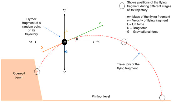
Figure 3.
Basic forces acting on flying fragment [24].
The authors further highlighted the interplay of inertia, launch velocity, mass and cross-sectional area of the fragment, and D in governing the travel distance of flyrock. It was suggested that additional research is required to refine the equations by integrating a more precise drag coefficient. Subsequently, a second article [24] was published on this topic in which a novel technique of enhancing the accuracy of the determined drag coefficient for flyrock was detailed. The calculation of the drag coefficient involved an analysis of the fragment’s movement at terminal velocity. However, it was discovered that the drag coefficient did not produce a unique value, possibly due to the influence of the fragment’s shape, size, launch velocity, and Ɵ. In the third article, the authors developed an adaptive system that could predict the launch velocities of flyrock using a 19-8-6-1 architecture Artificial Neural Network (ANN) [25] optimized with a fuzzy algorithm. The predictor demonstrated promising potential in predicting the initial velocity of flyrock fragments. However, it was noted that the predictor was still a concept due to the limited diversity of data resulting from the similar geological conditions at the investigated mining sites. It was further suggested that this limitation could present an opportunity for research aimed at creating a universal prediction model.
Recently, Blair [26] proposed a probabilistic approach for predicting flyrock range using a detailed BA combined with a mechanistic MCS based on investigational data from six surface mines. The approach involved wind tunnel experiments to determine variable coefficients of drag and lift for each fragment considering the effect of usual winds on the flyrock range. The study presented a two-dimensional (2D) ballistic model that utilized a fourth-order Runge–Kutta scheme to integrate the equations of fragment motion under the variable drag and lift forces. The model predictions were then compared with the probabilities of excessive flyrock range obtained from MCS. Later, the 2D model was extended to a pseudo-three-dimensional (3D) model to examine the impact of prevailing winds and pit-surface topography. At last, a complete 3D model was developed to determine the flyrock range.
1.3. Artificial Intelligence and Softcomputing Approach
Over the last few years, researchers have employed various soft computing (SC) techniques to forecast flyrock distance, in addition to traditional empirical methods. As a pioneering effort towards implementation of AI techniques in flyrock prediction, Monjezi et al. [27] developed a back propagation ANN model with an 8-3-3-2 neuron topology. The model was used to predict the degree of rock fragmentation and flyrock resulting from blasting in an iron mine in Iran. The authors later proposed a hybrid neuro-genetic algorithm for predicting flyrock and back-break at the Sungun Copper Mine [28]. This involved a genetic algorithm to optimize various paramters of the neural network such as the number of neurons in the hidden layer, learning rate, and momentum. Subsequently, many research works included the integration of an ANN with various other algorithms such as the Fuzzy Interface System (FIS) [29], Particle Swarm Optimization (PSO) [30], Imperialist Competitive algorithm (ICA) [31], and Firefly Algorithm (FA) [32], among others, to overcome the limitations of classic ANN modeling in predicting flyrock distance in copper mines and aggregate rock quarries. Following this approach, an adaptive neuro-fuzzy inference system (ANFIS) was employed by Trivedi et al. [33] to estimate blast-induced flyrock distance with a dataset of 125 blasts from four different opencast limestone mines in India. They found that ANFIS outperformed ANN and MVRA as a predictive tool for complex flyrock distance prediction problems of opencast mines.
In an attempt to estimate flyrock distance at the Delkan iron ore mine in Iran, Faradonbeh et al. [34] constructed several GP and GEP models using a dataset of 97 observations, comprising five input variables and one output variable, and concluded that the GEP model was highly reliable to predict flyrock. An advanced version of ANN, known as a deep neural network (DNN) model, was developed by Guo et al. [35] to predict flyrock based on the data from 240 blast events at Ulu Thiram quarry, Malaysia, The study utilized a powerful optimization technique called whale optimization algorithm (WOA) to minimize the flyrock.
Recently, Lu et al. [36] developed an outlier robust ELM (ORELM) model to predict the distance of flyrock caused by blasting in three aggregate rock quarry sites in Johor, Malaysia, and recommended the use of evolutionary optimization algorithms such as PSO and GA to further improve the performance of the ELM and ORELM models during the training process. The study used a dataset of 82 bench blasts and compared the results with those from multiple linear regression (MLR) models to discover that ORELM models were more efficient for predicting flyrock than both ANN and MLR models. Further, Bhatawdekar et al. [37] applied a novel equilibrium optimization technique to the ELM to anticipate the extent of flyrock generated in 114 blasts conducted at an aggregate limestone quarry in Thailand. In addition, two hybrid prediction models, namely, PSO-ANN and PSO-ELM, were developed and all models were run ten times. Comparing the EO-ELM model to the other two, it outperformed them in average results and exhibited a superior convergence in 10 runs. Notably, the study’s applicability was limited to the site only and may not be generalizable for other geological settings. Table 1 presents a compilation of some of the latest implementations of AI and SC methods for the prediction of flyrock in surface mines, summarizing the utilized algorithms, predicted variables, and the quantity of datasets employed by various researchers.

Table 1.
Key research articles on the application of AI and SC techniques for predicting flyrock.
The literature suggests that empirical models have a tendency to be highly specific to the particular site for which they were developed, and the results obtained with empirical and statistics-based models have not been entirely acceptable due to the complex nature of blasting operations. As a consequence, these models cannot be employed as a generic approach for predicting flyrock. In a similar way, AI and SC approaches have been proposed to deliver site-specific solutions as may be observed from the literature review. Numerous researchers have posited that a combination of AI, BA, and statistical approaches may be beneficial for an expanded grasp of the complex task.
1.4. Significance and Scope of This Study
After an extensive examination of the existing literature, it became apparent that a majority of research on flyrock predominantly emphasized the estimation of the maximum range or distance that is achieved by a flying fragment. However, this approach of predicting flyrock distance has some inherent limitations as it is largely dependent on the precision of two basic tasks: to identify the concerned rock fragment as a flyrock, and to correctly specify the point of ejection of this identified fragment. The difficulty of these tasks increases, particularly when several benches are consecutively blasted, which is a ususal practice in large surface mines.
Hence, a modified strategy capable of delimiting the danger zone must be adopted that depends on flyrock launch variables in addition to the existing methodology of distance estimation. The study documented in this research paper was carried out to investigate the factors influencing flyrock launch velocity (vf) using a high-speed motion analysis of 79 full-scale production bench blasts at five distinct surface mines in India. A dataset containing 231 flyrock instances was anaylzed to develop a model for forecasting vf by integrating the motion analysis results with robust machine learning regression techniques. A projectile simulation experiment was also conducted to demonstrate the methodology of delimiting the danger zone for bench blasts using the predicted vf combined with different possible sets of launch circumstances.
2. Materials and Methods
2.1. Research Stages
In this research work, a systematic and rigorous approach was employed to investigate the flyrock launch phenomenon. The study followed a well-defined set of steps to ensure the reliability and validity of the findings. The flowchart in Figure 4 offers a concise representation of the research methodology employed.
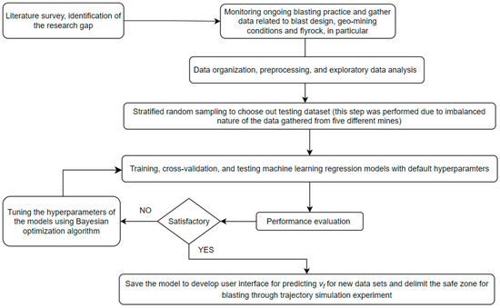
Figure 4.
Research steps followed in this study.
2.2. High-Speed Videography and Motion Analysis
High-speed videography and motion analysis is a widely used technique for the analysis of blast events. The process involves capturing a high-speed video of the blast event using specialized video cameras capable of recording at very-high frame rates. Typically, high-speed video (HSV) cameras have the capability to capture moving images with frame rates exceeding 250 frames per second (fps) [49]. The information obtained from high-speed video analysis can provide important insights into the behavior of the blast event monitored and can be used to optimize blasting designs and improve safety measures. High-speed motion analysis enables accurate identification of detonator timings, fragmentation, venting, fume generation, and flyrock [50,51]. The captured video is then analyzed using motion analysis software (MAS) v.0.9.5 that allows for the measurement and analysis of various parameters and enables researchers and practitioners to gain a deeper understanding of the physics of blast events. MAS uses advanced image-processing algorithms to extract relevant information by transforming the image pixels into the desired real-world units. In this study, the flyrock fragments ejected from the blastholes were observed with a HSV camera, as shown in Figure 5, and recorded at a rate of 500 fps. For analysis of the recordings, an open-source MAS Kinovea v.0.9.5 was used.
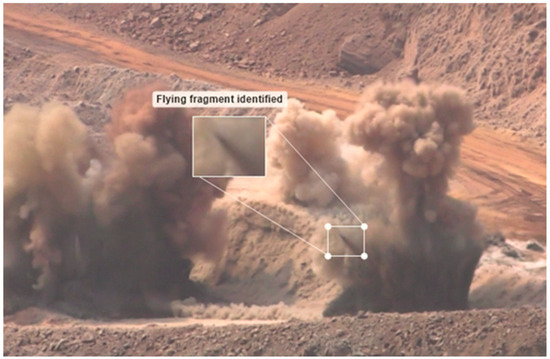
Figure 5.
Observing and identifying a flyrock fragment being launched using an HSV camera.
During motion analysis, it is desirable for the two-dimensional (2D) plane of motion to be orthogonal to the optical axis of the HSV camera. However, due to different spatial constraints at the mines regarding the location of the camera, ensuring orthogonality was not always possible. In such cases, to ensure minimal error in the measurements, the HSV scenes were calibrated using the ‘plane-calibration’ function in the MAS, which establishes a mapping between the pixels in an image and transforms the image coordinates to the corresponding real-world coordinates on a 2D plane and adjusts the pixels of the image using the calibrated coordinate system [15] as shown in Figure 6.

Figure 6.
Perspective calibration of the scene carried out before motion analysis using an adjusted coordinate system.
For the measurement of flyrock velocity, all the visible flying fragments were identified, and their launch site, angle, and velocity were measured one by one by marking the positions of the fragment over successive frames for an initial trajectory path, as shown in Figure 7.

Figure 7.
Measuring velocity and launch angle of an identified flying fragment over the initial trajectory.
Velocities measured on the initial trajectory path were averaged and noted as the vf for that particular fragment. For determining the launch angle (Ɵ) an angle measurement tool in the MAS was used. Additionally, the distance reached by the flying fragments was measured with the help of geographical coordinates obtained from a hand-held GPS device which was used for validation of the danger zone prediction. To obtain a wider range of launch circumstances as the input for the modeling process [25], flyrock generated from 231 blastholes were recorded during the study, in which 79 full-scale bench blasts (with a total of 4110 blastholes) were monitored during the period 2018–2022.
2.3. Machine Learning Regression
For analyzing the interactions between dependent and independent variables, multivariable regression analysis (MVRA) has been frequently used in research works related to geosciences, especially blasting operations [5,50,52]. However, this approach assumes a linear relationship between variables, which may not yield accurate results in this domain. On the other hand, alternative methods such as polynomial regression can model the complex interactions by incorporating higher-order terms but can lead to overfitting if the degree of the polynomial is too high. Therefore, for more accurate modeling of the complex, intricate relationships, non-linear multivariable regression (NLMR) approaches must be considered. During a comprehensive review of the literature related to modeling of complex non-linear problems in geotechnical and mining engineering, it was discovered that machine learning facilitates fast and accurate predictive analysis as compared to the empirical and numerical modeling approaches. The research works related to the application of machine learning regression for prediction of flyrock have already been summarized in Table 1, and a careful assessment of the literature revealed that many researchers have utilized ANNs as a predictive tool for estimating flyrock distance. However, it is important to note that ANNs are highly sensitive to hyperparameter selection and tend to build complex networks that can overfit smaller datasets (similar to the data used in this study) with higher dimensionality [53,54]. The importance of exploring a variety of machine learning models, ranging from simple white box models to more advanced alternatives, has been demonstrated in recent studies [55,56,57]. This approach enables the assessment of the necessity of complex models and facilitates the development of highly accurate and efficient models.
Hence, with the aim to develop the best machine learning model that can ensure robust modeling and generate precise predictions for vf, a similar approach was adopted by conducting a preliminary evaluation of relatively simple regression models, which included Ridge Regression (RR), Lasso Regression (LR), Elastic Net Regression (ENR), Decision Trees Regression (DTR) and K-nearest neighbors (KNN) regression along with advanced black box regression models such as Support Vector Regression (SVR), Random Forest Regression (RFR), Adaptive Boosting Regression (ABR), Extreme Gradient Boosting Regression (XGBR), and Extremely Randomized Trees Regression (ERTR). The fundamental principles of the models are provided in the ensuing sub-sections.
2.3.1. Ridge Regression (RR), Lasso Regression (LR), and Elastic Net Regression (ENR)
In the course of training and evaluating machine learning models, often the error resulting from either the training or testing dataset or both exceeds the anticipated level, which causes overfitting. A model is said to be overfitted when it performs exceptionally well on the training set but fails to generalize effectively to the unseen instances, leading to elevated error values. This could probably happen due to several reasons, one of which is the bias–variance trade off. Oversimplified models characterize high bias, while the inability of a model to generalize to unseen data signifies high variance. As bias is reduced, the model becomes more vulnerable to high variance and, conversely, when variance is decreased, bias may increase. Therefore, achieving a good predictive model necessitates striking a trade off or balance between these two measures. Regularization is an approach that addresses this issue and offers better performance in handling multicollinearity and overfitting. In regularization, the least-squares regression cost function (Equation (4)) is modified by adding a penalty term that penalizes large model coefficients and increases the generalizability. In the cost function, is the model coefficient or intercept, is the estimate of the true parameters, and is the actual value of the target variable calculated on from a dataset containing ‘n’ instances.
Popular regularization techniques in regression include Ridge Regression (RR), Lasso (Least Absolute Shrinkage and Selection Operator) Regression (LR), and Elastic Net Regression (ENR). RR is characterized by a penalty term, which incorporates half the square of the ‘L2’ norm and is added to the cost function [58,59]. The L2 norm encompasses the sum of squared differences between predicted and target values over the feature vector and this formulation imposes a constraint on the learning algorithm, compelling it not only to fit the data but also to minimize the model weights. The amount of ridge regularization is determined by the shrinkage hyperparameter ‘λ’, and its proper selection is crucial. When λ is equal to zero the RR becomes equivalent to linear regression. Conversely, when λ is exceedingly large, all the weight values converge to nearly zero, leading to an underfitted model. The cost function of LR is as shown in Equation (5).
On the other hand, instead of half the square of L2, the LR uses ‘L1’ norm as penalty term in the cost function. L1 norm is the sum of the absolute values of the difference between actual and predicted target values over the feature vector and is also known as the Manhattan distance (Equation (6)). In LR, λ operates similar to that in RR but a fundamental distinction lies in the treatment of coefficients. While both the techniques shrink the coefficients towards zero, LR is unique in that it assigns them exactly to zero when shrinkage reaches a certain threshold. Consequently, this leads to the creation of a model with a selected subset of features, rendering it considerably more interpretable and manageable in practice, particularly for datasets with several input features [58,60,61].
In contrast, ENR can be considered as a hybrid approach, combining characteristics from RR and LR. The penalty term in ENR comprises a blend of absolute-value and squared-value penalties. By integrating the penalties, ENR aims to capitalize on the strength of both techniques as shown in Equation (7) [55,58,62]. The degree of mixture is, however, controlled by the ratio hyperparameter (α). Specifically, when α = 0, ENR is effectively equivalent to RR and when α = 1, it aligns with LR.
2.3.2. K-Nearest Neighbors (KNN) Regression
KNN is a non-parametric supervised machine learning algorithm which employs the concept of feature similarity to predict the values of new data points. It can be effectively applied to both regression and classification tasks and its operation relies on majority voting, where the predicted output is the average of the predictions made by the K-nearest neighbors [63,64]. In the process of regression, the new data point is assigned a value based on its resemblance to the points in the training set. To achieve this, the algorithm first calculates the Euclidean or Manhattan distance between the new point and each training point and then selects the closest ‘k’ data points known as k nearest neighbors based on this distance [65,66]. The weighted mean of the outputs of the selected k nearest neighbors is the final prediction of the new point.
2.3.3. Support Vector Regression (SVR)
SVR is a versatile machine learning regression technique developed by Vladimir Vapnik [67] and is one of the derivations of Support Vector Machines (SVMs), the other being Support Vector Classification (SVC). The technique has gained widespread applications as a benchmark method in solving complex linear and non-linear regression [47,68,68,69]. The mathematical principle underlying SVR is based on the concept of finding an optimal hyperplane of the form of Equation (8), where, is a high-dimensional kernel input feature space, ‘ω’ is the weight coefficient, ‘T’ is the coefficient of variable transformation, and ‘b’ is the model error that best fits the given data points in a continuous space by minimizing the prediction error and maximizing the margin between the hyperplane and the closest data points known as the support vectors.
The formulation of SVR involves solving an optimization problem to find the hyperplane parameters that minimize the prediction error while also satisfying a set of constraints. For a given dataset of sample size ‘n’, the objective function of an SVR is typically formulated as shown in Equation (9) and subject to the constraints given in Equation (6), where ‘yi’ and ‘f(xi)’ are the actual and predicted values of the output variable for the ith data point ‘xi’, ‘ε’ is the marginal error, ‘C’ is a regularization parameter used for harmonizing the flatness and errors of the model, and ‘ξi’ and ‘ξi*’ are positive slack variables used for governing the distance between the actual and boundary values.
The loss function is further evaluated using Lagrangian multipliers and along with Karush–Kuhn–Tucker conditions to obtain the optimal solution. With this step, the equation of hyperplane gets transformed into Equation (10), where is a kernel function that is used to map the input parameters to the feature space.
The task of finding the optimal hyperplane is accomplished by using problem-specific kernel functions. SVR supports a variety of kernel types, such as linear, polynomial, Gaussian or Radial Basis Function (RBF), and sigmoid, but the choice of kernel relies largely on the specific problem and characteristics of the data [70,71]. In this study, a preliminary evaluation of the SVR with different kernel types was performed using the collected dataset and the Gaussian kernel expressed as in Equation (11) yielded the best results and was chosen for further analysis and improvement of the SVR model.
Figure 8 shows a conceptual depiction of a non-linear SVR.
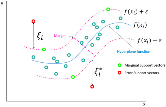
Figure 8.
Basic concept of a non-linear SVR.
2.3.4. Decision Trees Regression (DTR)
DTR is a supervised machine learning algorithm that involves constructing regression models in the form of a tree structure known as Decision Trees (DTs). DTs are widely used for both regression and classification tasks, with an objective to create a predictive model that estimates the target variable’s value using straightforward decision rules derived from the data features [5,72]. Conceptually, a tree approximates the data with piece-wise constants. A given dataset is partitioned into smaller subsets and a DT is developed accordingly, comprising decision nodes and leaf nodes. The root node, representing the best predictor, initiates the tree. The feature space is iteratively split into distinct regions to group similar target values together. The choice of split is determined by the mean squared error in regression problems. While building a DT, the process employs recursive binary splitting for the expansion of an extensive tree based on the training dataset. The expansion halts solely when each terminal node contains a quantity of observations that is below a specified minimum threshold. Recursive binary splitting is an iterative, top–down strategy utilized with the objective of reducing the residual sum of squares denoted as ‘ε’. This approach is applied to a partitioned feature space characterized by ‘m’ partitions, as outlined in Equation (12).
DTR models are easily interpretable white box models which can also be visualized. They require minimal data processing and are robust to the effect of outliers [73]. However, DTR models may generate highly complex trees that may tend to overfit the data and this necessitates the pruning of the trees and tuning of hyperparameters such as maximum depth or minimum samples. Furthermore, with complex intricate relationships, DTR are prone to high variance and biased trees with an unbalanced dataset with dominant classes. Therefore, DTR models are sometimes referred as weak learners [74,75]. Usually, to overcome these limitations and to increase the generalizability of the predictive models, a strong ensemble of several weak learners is created by training them either independently in parallel and combining the predictions through bootstrap aggregating (as in the Random Forest Regression and Extremely Randomized Trees Regression) or sequentially through boosting (as in Adaptive Boosting Regression and Extreme Gradient Boosting Regression).
2.3.5. Random Forest Regression (RFR)
RFR is an ensemble machine learning technique based on the concept of bootstrap aggregation or bagging. It consists of a combination of decision tree predictor models in which random subsets of the training dataset are provided to the individual decision trees by bootstrapping for training [5,76,77]. For example, let Dtr represent a set of given training data consisting of ‘N’ evidence, such as {(X1, Y1), (X2, Y2) (X3, Y3) … (XN, YN)}, where each piece of evidence consists of a set of input vectors ‘X’ with ‘m’ input features represented as {x1, x2, x3, … xm}, and a target variable ‘Y’. During bootstrapping, ‘n’ random subsamples (dtr) are drawn with replacement from ‘Dtr’ and the input data gets split at each node by the decision tree algorithm [78]. The root node initiates the splitting process, where each succeeding node applies its own function to divide the new input. Splitting progresses repetitively until a terminal node, referred to as ‘leaves’, is attained. When the training is complete, a prediction function such as the one shown in Equation (13) is constructed corresponding to each ith tree. The outputs of ‘n’ trees are then averaged in the case of regression problems. This process is called aggregation and is obtained using Equation (14) for a random forest regression model.
However, sometimes one or more of the ‘m’ features get chosen in many of the ‘n’ trees if they are good predictors of the output variable (Y), leading to their correlation. To avoid such correlation of different trees and provide immunity to noise, the modified tree learning algorithm used by random forests chooses a random subset of the features at each root node split during the learning process by feature bagging. Accordingly, with several de-correlated trees, the diversity of trees can be increased, and the noise sensitivity of the model gets largely decreased, making it robust against slight variations in the input data. With RFR, the trees grow without pruning, and this makes the algorithm computationally less expensive. Usually, the more trees that are grown in a forest, the more reliable and accurate a prediction can be. In open-pit bench blasting, the Random Forest method has been used by different researchers for the prediction of back-break, flyrock, and air overpressure in bench blasting [77,79,80,81]. Figure 9 shows a basic architecture of an RFR algorithm.
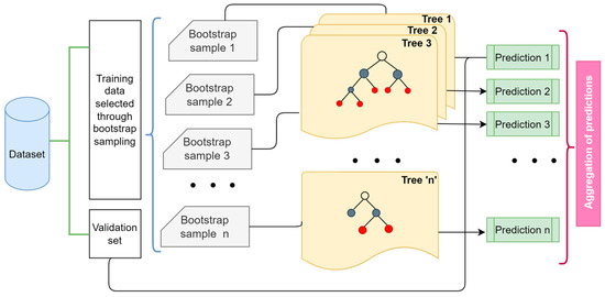
Figure 9.
Basic architecture of an RFR algorithm.
2.3.6. Extremely Randomized Trees Regression (ERTR)
ERTR is a model based on a bootstrap aggregation ensemble of several decision trees (DT) and was first introduced by Geurts et.al [82]. In contrast to the RFR, where DT are constructed using bootstrap samples, each base learner in the ERTR is trained on the complete dataset. Like RFR, ERTR divides nodes using random subsets of input features; however, it differs in the way it selects the optimal split [82,83]. ERTR chooses the split randomly, whereas RFR selects the best split from a random subset of input features at each node. The hyperparameters used for ERTR are similar to those of RFR [84].
2.3.7. Adaptive Boosting Regression (ABR)
In contrast to the bagging ensembles, the boosting ensemble technique aims to combine the output of multiple weak learners in a sequential manner to create powerful model with enhanced predictive capabilities compared to individual base learners [38]. Adaptive boosting, commonly known as Adaboost, was introduced by Freund and Schapire to improve the performance of DT [85]. In Adaboost, DTs are grown sequentially, with each subsequent model attempting to rectify the error made by its predecessors. This is achieved by assigning higher weights to data points that were improperly handled by previous models [86]. Initially, all data points in the training dataset containing ‘n’ number of samples are assigned equal weights ‘’, and then the first base learner ‘t’ is trained.
Predictions made by the first base learner ‘t’ are assessed and the loss ‘’ is calculated for the ith sample, as shown in Equation (15) and subject to Lt ϵ [0, 1]. Thereafter, average loss for all the predictions made by the weak learner ‘’ is calculated and the weights are updated for the next iteration as shown in Equations (16) and (17).
where βt is the information gain achieved at the last weak learner and is expressed as the ratio given in Equation (18).
The boosting algorithm then proceeds in the same manner through ‘T’ iterations until the ‘tth’ trained base learner is reached and a cumulative prediction with minimum error is obtained.
2.3.8. Extreme Gradient Boosting Regression (XGBR)
XGBR is also an ensemble machine learning algorithm based on the principle of gradient boosting. In the gradient boosting technique, multiple weakly predictive models, which are usually decision trees, are combined to create a stronger ensemble model [87]. The algorithm efficiently handles both classification and regression tasks by generating and working with boosted trees in parallel [75]. The core concept of the XGBR is its objective function which is defined based on the conditions of gradient boosting. For a given dataset D = {(xi, yi)} comprising of ‘n’ samples and ‘m’ features, ‘z’ additive functions fz(xi), such that space of regression trees, are utilized to approximate the predictions made by the ensemble model, as shown in Equation (19).
Later, to optimize the ensemble tree and reduce errors, the objective function (Equation (20)) of the XGBR is minimized, where ‘l’ is the convex loss function utilized to quantify the disparity between actual and predicted values of the target variable and is the regularization term. This process is repeated for ‘t’ iterations.
In the regularization term, serves as the penalty factor to account for the complexity of the regression tree approach and it is calculated using Equation (21), with the regularization shrinkage parameter ‘λ’ and pruning penalty constant ‘’ to control the complexity of the model and prevent overfitting.
In each of the successive weak tree learners, the prediction error of the prior model is corrected with the goal of finding an optimal output value () at the leaf node and can be expressed as the ratio of the first and the second derivative of the loss function known as the gradient and the hessian, respectively. The loss function is then solved using second-order Taylor’s approximation. At every split, the optimal output value is determined by equating the loss function to zero and then the XGBR evaluates split gain (G) to determine the improvement. Split gain is calculated using similarity scores (S) at the root and the leaf nodes using G = SLL + SRL − SR, where ‘SLL’, ‘SRL’, and ‘SR’ are the similarity scores computed using Equation (22) for the left leaf node, right leaf node, and root node, respectively [74,88].
The procedure is iteratively repeated until reaching the terminal node, where the prediction ‘Ti’ associated with this specific terminal node is multiplied by the learning rate ‘ε’. The resulting value is then added to the previous prediction, effectively enhancing and boosting the predictive power of the model at each successive step, as shown in Equation (23). The fundamental structure of an XGBR model is shown in Figure 10.

Figure 10.
Fundamental structure of an XGBR model.
2.4. Hyperparamters Tuning
Hyperparameters of a machine learning model are configuration settings made by the user before training and remain fixed throughout the training process. These settings are the controlling parameters that regulate the behavior of the model and influence its performance and learning process. Optimizing hyperparameters leads to improved generalization and better performance on unseen data, helps in the efficient utilization of computational resources, and saves time by finding the right balance between overfitting and underfitting [89]. The process of hyperparameter optimization aims to find the best set of hyperparameters, ‘x*’, which minimizes an objective score (usually the root-mean-squared error) ‘f(x)’ evaluated using the validation set. The mathematical representation of the process is shown in Equation (24), where the set of hyperparameters ‘x’ can be any value chosen from a wide range of values in the hyperparameter space ‘χ’.
However, the challenge lies in the elevated computational cost associated with evaluating the objective function. Each attempt with different hyperparameters necessitates the training of the model on the training dataset and predictions on the validation data. This process becomes very time-consuming, especially when dealing with numerous hyperparameters or complex models such as ensembles and deep neural networks. In such situations where manual optimization becomes infeasible and extremely complex, automated hyperparameter tuning provides a better alternative solution. Different methods of automated tuning include grid search, randomized search, evolutionary algorithms, and stochastic algorithms such as Bayesian optimization (BO). Of these, grid and randomized searches normally consume a lot of time analyzing the bad hyperparameters, since the processes are completely uninformed about the prior evaluations. On the other hand, evolutionary algorithms require a large number of iterations to converge and can be computationally expensive. Therefore, in this study, BO was used as the technique for tuning the hyperparameters of the regression models.
Bayesian Optimization (BO)
In BO, firstly, a probabilistic surrogate model that represents the objective function is created by employing one of three main types: the Gaussian process, sequential model-based algorithm configuration (SMAC), and tree Parzen estimator (TPE) [60]. Then, by obtaining the projected distribution of this probabilistic surrogate model, an acquisition function accomplishes the allocation of evaluation points by balancing the trade-off between the sampling instances from unexplored areas and the sample data points from the regions likely to contain the global optimum based on the posterior distribution. This enables continuous refinement of the search space and guides the selection of hyperparameter configurations. The selected hyperparameter values are then evaluated on the actual objective function, and the iterations are performed until the maximum threshold is reached. For tuning the regression models in this research work, the Gaussian process surrogate model [90] was used, which is predominantly employed for optimizing continuous variables. Assuming that ‘f(x)’, defined earlier, is a realization of the Gaussian process and has a mean ‘μ’ and covariance ‘σ2’, and the predictions follow a normal distribution as shown in Equation (25).
Furthermore, an acquisition function based on expected improvement (EI) (Equation (26)) was used, which is the expected value of an improvement function defined in Equation (27), where, ‘φ(z)’ is the probability density function of the normal distribution. N (0, 1).
Further, the time complexity of an algorithm measures the computational time required for the algorithm to run as a function of the input size. While the actual time taken may be influenced by the hardware, operating system, and processors of the machine, the analysis of time complexity focuses solely on the execution time of the algorithm. In analyzing the algorithms, the commonly used parameter is the ‘O-notation’, which provides an upper limit to the execution time, specifically in the worst-case scenario. BO with a Gaussian process surrogate model has a cubic complexity for a dataset with a sample size of ‘n’, and its time complexity is, therefore, O(n3) [91]. In this experiment, the sample size was smaller; the optimization algorithm performed fairly well with greater efficiency, lasting no longer than 5.16 s/iteration for any of the models on a machine having an Intel core-i5 8th generation processor and 8 gigabytes of random-access memory (RAM).
3. Field Data Acquisition and Processing
3.1. Site Description and Blasting Practice
The research work reported in this paper employed a dataset comprising 231 blastholes that generated flyrock during 79 full-scale blasts (with a total of 4110 blastholes) conducted at five distinct surface mines in India, each identified by a unique code name for the purpose of this study: Mine A, Mine B, Mine C, Mine D, and Mine E. Of these, mines A and B were situated in the Jharia Coalfields region and consist of a Barakar formation overburden rock. Mine C was located in Singrauli coalfields and encompasses a Lower Gondwana Barakar formation overburden rock. Mine D was an iron ore mine from the Chilpi formation belonging to the iron ore series of the Dharwarian system of the Pre-Cambrian or Archean age. Lastly, Mine E comprised the flaggy limestone of the Raipur group. For examining the physicomechanical characteristics of the predominant rock formations at the selected sites, a variety of rock specimens were collected and prepared for laboratory testing. The prepared rock samples were subjected to a series of laboratory tests following the recommended methods [92] by the International Society for Rock Mechanics (ISRM). Each test involved a minimum of ten samples, and the resulting data were utilized to determine the average values. The findings of these tests are summarized in Table 2.
Table 2.
Results of the tests to determine physicomechanical properties of the rock mass specimen.
In each blast conducted, blastholes were drilled following a staggered pattern and loaded with fully coupled column charges of bulk site mixed emulsion (SME) explosives. The final cup density (ρe) of the explosives ranged from 1.03 g/cm3 to 1.28 g/cm3, while the confined in-hole velocity of detonation (cdc) ranged from 4328 m/s to 4899 m/s. For mitigating the scattering effect on nominal delay intervals, electronic initiation with digital detonators was employed in all the blasts. Comprehensive data were collected, including information on parameters such as B, S, q, ls, d, ρe, ρr, cdc, linear charge concentration (qlc), explosive energy content (We), linear energy concentration (Wlc), bench height (Hb), flyrock launch velocity (vf), flyrock range (Rmax), and Ɵ. It is worth noting that the variables summarized herein are specifically those utilized for predictive modeling and analysis. Notably, q has commonly been employed by many researchers for predicting flyrock. However, considering the potential variations in energy content due to differences in density and manufacturing among suppliers, the energy factor (W) was utilized as a predictor variable instead of the traditional powder factor. The value for W was calculated using the equation W = q × We, allowing for the inclusion of varying energy content in the predictive modeling process.
3.2. Exploratory Data Analysis
Prior to the modeling process, exploratory data analysis was carried out to derive insights about the dataset. Since the size of sample was greater than 30, the assumption for normality was relaxed [50]. The strength of the linear relationship between the output and the input variables was measured using Pearson’s correlation coefficient ‘r’ and a correlogram was plotted, as shown in Figure 11. A rule-of-thumb given in Equation (28) was utilized to determine the strength of correlation, where ‘n’ represents the sample size, and thus an absolute value greater than or equal to 0.23 was considered a good linear correlation.

Figure 11.
Correlogram showing Pearson’s correlation between the input variables and the output.
It may be observed from the correlogram that ρr had a very strong relationship with vf, followed by S, B/d, W, B, ls/B, and Wlc. Although S and B were strongly correlated with the output variable and have been used by many researchers as influencing factors for predicting flyrock distance, there is hardly any information in the literature signifying the direct effect of S on vf. Hence, for the development of predictive models B, B/d, ls/lbh, ls/B, ρr, and W were finalized as the input variables. Descriptive statistics of the dataset are summarized in Table 3, and the standardized distribution of the variables can be observed from the box-and-whisker plot shown in Figure 12.
Table 3.
Summary of the sample dataset used in this study.
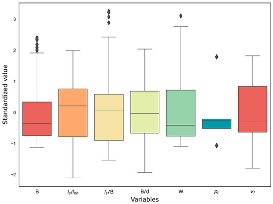
Figure 12.
Distribution of the variables in the dataset.
3.3. Evaluation Criteria
Evaluation criteria are a crucial step in assessing the performance and predictive accuracy of regression models. Many researchers have recommended considering multiple evaluation metrics to gain a comprehensive understanding of the models’ performance and to make informed decisions in regression analysis. The criteria for model evaluation were based on utilizing the key performance metrics used in most of the recent studies on the development of machine learning regression models. For this purpose, the coefficient of determination (R2), root-mean-squared error (RMSE), mean absolute error (MAE), mean absolute percentage error (MAPE), index of agreement (IA), and Kling–Gupta Efficiency (KGE) were calculated for training and testing datasets using the formulae given in Equations (29)–(34), where, ‘r’ is the Pearson’s correlation coefficient, ‘α’ is the measure of variability, ‘β’ is the bias, ‘yi’ is the actual value, ‘’ is the predicted value, and ‘’ is the mean of ‘N’ observations.
The R2 score of a model quantifies the fraction of the variability in the dependent variable that is accounted for by the independent variables within the model. Its value ranges from 0 to 1, where values closer to 1 indicate a better fit. On the other hand, RMSE calculated the average magnitude of the residuals (difference between the observed and the estimated values) by taking the square root of the mean of squared residuals. It provides a measure of the average prediction error, with lower values indicating better prediction accuracy. The advantage of RMSE is that it has the same unit of measurement as that of the dependent variable. In contrast to RMSE, MAE calculates the mean absolute disparity between predicted and actual values, representing a quantitative measure where smaller values signify superior outcomes. MAPE expresses the average percentage deviation between the actual and predicted values, and a lower MAPE value indicates a more accurate model. IA was introduced by Willmott [93] and is a standardized gauge of model prediction error whose value ranges from −∞ to 1. It is calculated as the ratio of mean-square error to potential error; an IA value of 1 signifies perfect correspondence while values closer to zero and negative values denotes poorer agreement. This index can identify additive and proportional discrepancies in observed and simulated means and variances. On the other hand, KGE is a goodness-of-fit metric, which was formulated by Gupta et al. [94] and modified by Kling et al. [95] to prevent cross-correlation between bias and variability ratios. It offers a diagnostic decomposition of MSE and similar to the R2 score, a higher value of KGE is an indicator of higher accuracy.
4. Development of Predictive Models
4.1. Data Pre-Processing and Exploring Machine Learning Models
In this study, machine learning regression models were developed using the Python v.3.9.12 programming language, and the sci-kit learn and Matplotlib libraries were primarily used. A stratified sample of 31 datapoints was meticulously created to serve as a separate testing dataset. This was carried out to obtain representative testing instances from the imbalanced data obtained due to significant differences in the geotechnical and geological properties of the rock masses at the sites studied. The remaining 200 instances were utilized for training the models. Standard scaling was used to address the issue of different scales or ranges of features by transforming the data such that it had a mean of 0 and a standard deviation of 1. A five-fold cross-validation approach was used for training and validation of the models [55]. Additionally, the effect of different kernels on the SVR [39] was also assessed by running it with default hyperparameters while changing the kernel type in each run. The results of the kernel experiment have been summarized in Table 4.
Table 4.
Results of the kernel experiment.
Based on the initial evaluation, it was observed that the SVR base model with RBF kernel performed better than other models. Therefore, it was set as the kernel for SVR in further experimental analyses. Further, using the machine learning regression approaches discussed in Section 2.3, ten regression models were developed using the default hyperparameters and a preliminary evaluation was carried out. The evaluation metrics of the base models for the training and testing phases have been summarized in Table 5.
Table 5.
Performance metrics for regression models trained with default hyperparameters.
4.2. Model Optimization by Tuning the Hyperparameters
The hyperparameters of the base models were tuned using the Bayesian Optimization algorithm. To accomplish this, a Python package named ‘bayes_opt’ was imported [96]. For guiding the search for optimal hyperparameters, the ‘Expected improvement’ acquisition function was utilized. The hyperparameter search space for the base models, along with their optimal values, are summarized in Table 6.
Table 6.
Hyperparameters [87,97] for the regression models.
During the optimization process, different combinations of hyperparameters were used for 300 iterations to ensure the proper convergence of the optimization process. The optimized models with the best hyperparameters were then trained and fit using the training data and evaluated with five-fold cross validation. Subsequently, the optimized models were then used to make predictions on the testing dataset and the respective metrics along with CI0.95 were computed and recorded. Out of the ten regression models, only six black box models demonstrated high accuracy levels. The convergence curves for these good performing regression models plotted using the ‘Minimum MSE’ as a criterion have been depicted in Figure 13, wherein it can be observed that the optimization process for all the models converged well.
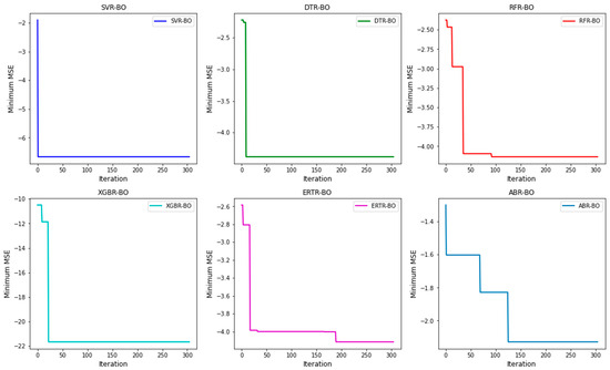
Figure 13.
Convergence graphs of BO plotted during the hyperparameter tuning of the six best performing machine learning regression models.
5. Results and Discussion
5.1. Prediction Accuracy of the Developed Regression Models
The values of the evaluation metrics obtained during the training and testing of the optimized regression models are presented in Table 7. The values of the training metrics represent the mean validation scores derived from the k-fold cross validation conducted during the training phase, whereas the test metrics were acquired through predictions made on the separate testing dataset reference earlier in this article.
Table 7.
Performance metrics for the optimized regression models.
The tabulated results revealed that the black box models (SVR-BO, DTR-BO, RFR-BO, ERTR-BO, ABR-BO, and XGBR-BO) exhibited superior performance across both training and testing phases compared to the white box models (RR-BO, LR-BO, ENR-BO, and KNN-BO). Among the four white box models, KNN-BO consistently outperformed its counterparts throughout training and testing. However, like the other three white box models, there was a significant difference between the training and testing R2 scores indicating a model overfit condition. Conversely, among the six black box models, the ensemble models (specifically, RFR-BO, ERTR-BO, ABR-BO, and XGBR-BO) demonstrated better performance than the single model SVR-BO. Notably, the performance of DTR-BO closely resembled that of SVR-BO. In the comprehensive model assessment, the most outstanding performance was observed for the ERTR-BO model, which achieved an R2 value of 98.8%, IA of 99.7%, and KGE value of 98.4% during the testing phase. This was followed by the testing R2 values of XGBR-BO (98.0%), RFR-BO (97.8%), and ABR-BO (97.0%). Furthermore, in terms of vf predictions on the testing dataset, ERTR-BO exhibited the lowest RMSE of 0.866 m/s, the lowest MAE of 0.517 m/s, and the minimal MAPE of 2.126%. This was visually evident in Figure 14, which portrays the actual versus predicted scatter plots for all the optimized regression models, highlighting the remarkable alignment of the ERTR-BO model’s predictions with the perfect predictions line.
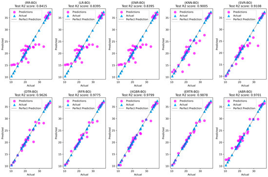
Figure 14.
Actual versus predicted scatterplots for all ten optimized regression models.
5.2. Model Interpretation Using SHAP
Developing complex black box machine learning models is a widely applied highly efficient technique to predict the target variable in mining and geotechnical engineering, particularly when the response variable is dependent on intricately related non-linear features. However, despite being remarkably proficient, these models suffer a significant constraint of being opaque and uninterpretable. This limitation associated with the black box models underscores the necessity to furnish a clarification of the generated outputs and the ramifications of the diverse input features on the resultant output. To address this, a model explanation framework called SHAP (Shapely Additive Explanations) was employed in this study [55,56,57]. SHAP analysis is derived from game theory and it encompasses strategic interactions among factors to allocate gains and costs equitably among collaborators. Although versatile, only a few studies have employed it to elucidate black box models [57,98,99].
The shapely value for feature i is calculated using Equation (35), with f as the black-box model and x as an input datapoint corresponding to a single tabular dataset row. Initially, all possible subsets z’ of the transformed input x’ are iterated to account for an interaction between individual feature values. Subsequently, the black box model output is determined for subsets with and without the feature of interest. The difference of indicates the marginal contribution of feature i. This process is repeated for each subset permutation, and weighting is calculated based on the total number of features, M. On the other hand, an emphasis is placed on small correlations to observe isolated feature effects on predictions [100,101,102].
In the conducted modeling experiment, the ERTR-BO model demonstrated exceptional proficiency in regression for the provided dataset. Given its tree-based nature, a tree-based SHAP explainer was employed to assess the impacts of distinct features on the predicted variable (vf) [101]. Figure 15 illustrates SHAP plots depicting global and local contributions through bar, dot, and force plots [102]. Feature names in the plots remain consistent with the study’s nomenclature, except for ‘rhor,’ which denotes ρr. In both the bar and dot plots, the vertical axes present input features based on their contribution to the vf prediction model. The dot plot’s horizontal axis (Figure 15a) showcases actual SHAP values, while the bar plot’s horizontal axis (Figure 15b) indicates the mean of absolute SHAP values. Each dot in Figure 15a corresponds to a SHAP value tied to a distinct dataset feature. The color transition from purple to pink within the dots signifies escalating SHAP value magnitudes.
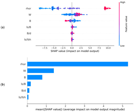

Figure 15.
SHAP summary plots showing relative feature importance in the ERTR-BO model: (a) dot plot, (b) bar plot, (c) force plot showing local explanation for a datapoint in the test dataset.
On the other hand, Figure 15c displays a force plot exemplifying the local contribution of a test dataset point. This plot revealed an actual prediction of 26.02 m/s, while the base value of 24.05 signified the expected value or mean of the predictions made for the whole dataset. Beneath the force plot, insights are provided into each feature’s contribution to the 26.02 m/s prediction.
Observing Figure 15, it was evident that the bulk density of rock (ρr) stood out as the foremost influential feature impacting the flyrock launch velocity, followed by the energy factor (W), burden (B), burden to blasthole diameter ratio (B/d), stemming length to burden ratio (ls/B), and ratio of the stemming length to the length of blasthole (ls/lbh), respectively. This phenomenon could be attributed to the influence of ρr on the strength of the rock mass which subsequently affects the degree of fragmentation and the momentum achieved by the detached fragment. The momentum acquired by the fragment of a given mass largely depends on the force exerted on it. This force is governed by the blasthole pressure generated due to post-detonation expanding gases. This depends on the energy content of the explosives and, thus, the higher the energy factor, the greater the momentum. This could be considered as the reason behind W being the second most influential feature after ρr. On the other hand, the burden directly influences the mass of the rock to be displace by explosive force, consequently shaping the momentum achieved by the detached rock fragments based on the interplay of energy and mass, thereby imparting the ensuing fragment velocity. The remaining three parameters, B/d, ls/B, and ls/lbh, indirectly signify this energy–mass interplay, denoted through blasthole volume and burden mass for blast-induced rock movement.
5.3. Development of a Graphical User Interface (GUI)
With the objective of enhancing the applicability of the established ERTR-BO model for the prediction of flyrock in real-world field scenarios, an attempt was made to develop a simple graphical user interface (GUI), which is depicted in Figure 16. The creation of this GUI involved the application of the ‘Tkinter’ Python library to provide a platform for the users to input the predictor variables and subsequently obtain the predicted flyrock velocity [103]. As depicted in the GUI illustration, the process commenced with the user inputting values for input parameters, including burden, stemming length to blasthole length ratio, stemming length to burden ratio, burden to blasthole diameter ratio, energy factor, and rock density. The flyrock launch velocity was then automatically calculated utilizing the optimized ERTR-BO model and presented in the predicted VF section. This predicted velocity could then be employed to carry out a simulation exercise for forecasting the flight trajectories and determining the potential maximum range of a probable flyrock occurrence, as demonstrated in the following sub-section.
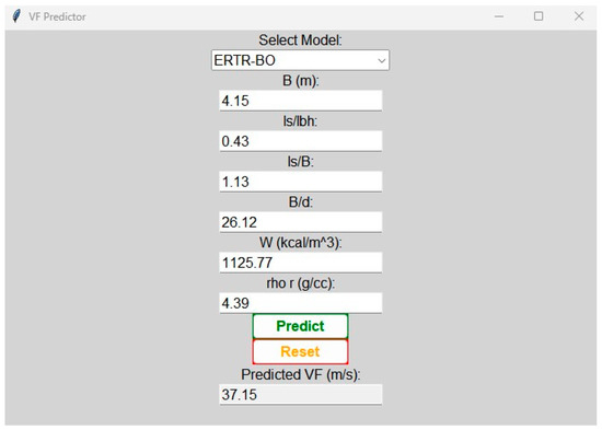
Figure 16.
Simple graphical user interface created for using the ERTR-BO model to predict vf.
5.4. Simulation of Flyrock Trajectories
In addition to blast design variables, flyrock is dependent on a range of uncontrollable factors, including the presence of discontinuities and other rock mass characteristics such as fissures and cracks. As a result, its occurrence remains unpredictable until the blast is executed. Therefore, a projectile simulation was carried out by utilizing vf prediction results on the testing dataset. In the experiment, the flight trajectories for the probable occurrence of flyrock were forecasted considering different possible launch circumstances. To ensure a conservative estimation for delimiting the danger zone at the investigated sites, the upper limit of CI0.95 for the predicted velocity was considered. Based on the principles of projectile motion, it was hypothesized that a flying fragment would reach its maximum range at an angle of 45°. Therefore, the same launch angle measure was used consistently throughout the simulations. The largest flyrock fragment observed in all the blasts had a mean diameter of 22 cm, so assuming a spherical shape, five different diameters of flyrock in the range of 5–25 cm were considered for simulation, and their corresponding masses were calculated following the approach suggested by Stojadinovic et al. [23]. For launch locations, both the bench top and bench face were considered, as cratering and rifling occur from the bench top, while face bursting occurs at the bench face. Consequently, the projectile simulations were conducted using fifteen unique combinations of five distinct fragment masses and three evenly spaced launch locations on the bench face measuring upwards from the toe. Table 8 details the specifics of the experimental data utilized for simulation and it contains a single entry as an example for demonstrating the experiment in this article. The drag coefficient was taken to be 0.08, and the acceleration due to gravity was set as 9.8 m/s2.
Table 8.
Sample instances for demonstrating the experimental set-up for projectile simulation.
The trajectories resulting from simulations for the 15 different combinations are depicted in Figure 17, showcasing the range and patterns of flyrock trajectories for one of the instances from Mine D as given in Table 8. The farthest range of flyrock for this particular case was predicted to be approximately 140 m, which may be observed from the simulated trajectories. However, in the particular blast, the actual range of the farthest flyrock fragment identified and measured using GPS coordinates was around 112 m. Moreover, it is worth noting that the accuracy of simulation should not be assessed by comparing the predicted range with the actual range of flyrock measured at the blast site due to two major reasons: first, the farthest fragment identified might not be that which is sampled in the demonstration data; and second, the simulation experiment has been conducted with certain assumptions regarding the launch angle, launch velocity, fragment shape, and drag coefficient, which are not necessarily the same in actual conditions. From this point of view, the over-prediction of range obtained from the simulation is fairly acceptable for ensuring the safety of men, materials, and equipment by delimiting the danger zone of the blast before executing it.
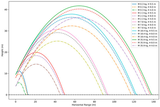
Figure 17.
Simulated trajectories of flyrock for fifteen different combinations of fragment mass and launch height for a blast from Mine D.
6. Conclusions
Flyrock generation remains a persisting safety concern in surface-mine blasting. It poses significant operational risks to people, machinery, materials, and structures nearby. Prevention of the occurrence of flyrock needs careful planning of the blast design parameters for efficient utilization of the explosive energy. In this research paper, a modified approach of delimiting the danger zone for bench blasting has been proposed. The method integrates a high-speed motion analysis and machine learning regression to help optimize the blast design variables, thereby reducing the chances of flyrock generation and risks associated with it. The study investigated the factors influencing flyrock launch velocity (vf) using high-speed motion analysis of 79 full-scale production blasts conducted with a total of 4110 blastholes at five distinct surface mines in India. Out of these, 231 blastholes generated flyrock. The data acquired through high-speed motion analysis were utilized to develop ten Bayesian optimized machine learning regression models. All the models were optimized using five-fold cross validation and their accuracy was rigorously examined. The conclusions drawn from the experiment are as follows:
- Out of the ten Bayesian optimized machine learning regression models, the optimized Extremely Randomized Trees Regression model (ERTR-BO) demonstrated the best predictive accuracy, exhibiting higher R2, IA, and KGE scores and the lowest RMSE, MAE, and MAPE;
- An in-depth analysis of the achieved accuracies of the white box models unveiled their inability to effectively capture the intricate and complex non-linear dependencies existing between the input features and the target variable. Furthermore, these models displayed evidence of overfitting, as indicated by a substantial disparity between the training and test R2 scores;
- Each of the ensemble black box models exhibited notably superior predictive capability as compared to the black box single model SVR-BO;
- Through the application of Bayesian optimization, the R2 score of SVR demonstrated notable enhancement with an increase of 15.04% for the training set and 14.12% for the test set, followed by improvements in the ENR (13.09%-training, 12.20%-testing), LR (3.85%-training, 6.26%-testing), KNN (2.08%-training, 2.76%-testing), and ABR (1.36% training, 1.38%-testing). Certain other black box models performed well with their respective default hyperparameters. Notably, there were no discernable improvements in the RR scores even after hyperparameter tuning;
- The SHAP analysis, undertaken to elucidate the marginal contribution of input features in predicting vf by the ERTR-BO model, unveiled ρr as the most influential feature, followed by W, B, B/d, ls/B, and ls/lbh. The analysis further substantiated the tangible significance and intricate interactions among these features that collectively contributed to the generation of flyrock in bench-blasting operations;
- In order to improve the practicality of the ERTR-BO model for real-world flyrock prediction, a simple GUI was designed. The interface may allow users to input predictor variables and obtain predicted flyrock velocity. This velocity may then be used for simulating flight paths and estimating the potential range of flyrock events, as demonstrated in Section 5.4.
The generation of flyrock is influenced not only by blast design variables, but also by uncontrollable factors such as site-specific geo-mining conditions and the physicomechanical properties of the rock mass to be blasted. As a result, the unpredictability of flyrock persists until the occurrence of the actual blast, which is a contributing factor to the limited data availability for this study. Additionally, it is important to acknowledge that generating more flyrock-related data is not feasible, given that flyrock is an undesirable hazard rather than a production activity, and capturing the flyrock phenomenon necessitates extensive field observation for prolonged periods. The model developed in this study has the potential to serve as a valuable tool for field engineers in refining the blast design variables during planning of bench blasts in addition to the reliance solely on distance forecasting methodologies. The utility of this approach is particularly relevant in situations where advanced and costly equipment, such as a high-speed video camera, is not available. The model also holds the potential to mitigate the hazards of blast-induced flyrock that can arise in construction and maintenance sites which, unlike mines, are typically situated amidst human settlements and urban conglomerates. Moreover, this approach can serve as a mechanism to proactively mitigate disturbances originating from the vicinity, which in turn can alleviate significant compensatory expenditures incurred by the mine or construction site management.
Author Contributions
Conceptualization, R.M., A.K.M. and B.S.C.; data curation, R.M.; formal analysis, R.M.; investigation, R.M.; methodology, R.M.; supervision, A.K.M. and B.S.C.; validation, R.M.; visualization, R.M.; writing—original draft, R.M.; writing—review and editing, R.M., A.K.M. and B.S.C. All authors have read and agreed to the published version of the manuscript.
Funding
This research received no external funding.
Institutional Review Board Statement
Not applicable.
Informed Consent Statement
Not applicable.
Data Availability Statement
Not applicable.
Acknowledgments
The authors would like to acknowledge the support provided by the Department of Mining Engineering, IIT (ISM), Dhanbad for carrying out this research.
Conflicts of Interest
The authors declare no conflict of interest.
References
- Bhandari, S. Engineering Rock Blasting Operations; Taylor & Francis: Abingdon, UK, 1997; ISBN 9789054106586. [Google Scholar]
- Adhikari, G.R. Empirical Methods for the Calculation of the Specific Charge for Surface Blast Design. Fragblast 2000, 4, 19–33. [Google Scholar] [CrossRef]
- Ghasemi, E.; Sari, M.; Ataei, M. Development of an Empirical Model for Predicting the Effects of Controllable Blasting Parameters on Flyrock Distance in Surface Mines. Int. J. Rock Mech. Min. Sci. 2012, 52, 163–170. [Google Scholar] [CrossRef]
- Agrawal, H.; Mishra, A.K. Probabilistic Analysis on Scattering Effect of Initiation Systems and Concept of Modified Charge per Delay for Prediction of Blast Induced Ground Vibrations. Measurement 2018, 130, 306–317. [Google Scholar] [CrossRef]
- Kumar, S.; Mishra, A.K.; Choudhary, B.S. Prediction of Back Break in Blasting Using Random Decision Trees. Eng. Comput. 2022, 38, 1185–1191. [Google Scholar] [CrossRef]
- Armaghani, D.J.; Koopialipoor, M.; Bahri, M.; Hasanipanah, M.; Tahir, M.M. A SVR-GWO Technique to Minimize Flyrock Distance Resulting from Blasting. Bull. Eng. Geol. Environ. 2020, 79, 4369–4385. [Google Scholar] [CrossRef]
- Raina, A.K.; Murthy, V.M.S.R.; Soni, A.K. Flyrock in Bench Blasting: A Comprehensive Review. Bull. Eng. Geol. Environ. 2014, 73, 1199–1209. [Google Scholar] [CrossRef]
- Jimeno, E.L.; Jimino, C.L.; Carcedo, A. Drilling and Blasting of Rocks; Taylor & Francis: Abingdon, UK, 1995; ISBN 9789054101994. [Google Scholar]
- Little, T.N. Flyrock Risk. Australas. Inst. Min. Metall. Publ. Ser. 2007, 35–43. [Google Scholar]
- Kecojevic, V.; Radomsky, M. Flyrock Phenomena and Area Security in Blasting-Related Accidents. Saf. Sci. 2005, 43, 739–750. [Google Scholar] [CrossRef]
- Monjezi, M.; Dehghani, H.; Singh, T.N.; Sayadi, A.R. Application of TOPSIS Method for Selecting the Most Appropriate Blast Design. Arab. J. Geosci. 2012, 5, 95–101. [Google Scholar] [CrossRef]
- Lundborg, N.; Persson, A.; Ladegaard-Pedersen, A.; Holmberg, R. Keeping the Lid on Flyrock in Open-Pit Blasting. Eng. Min. J. 1975, 176, 95–100. [Google Scholar]
- Jahed Armaghani, D.; Tonnizam Mohamad, E.; Hajihassani, M.; Alavi Nezhad Khalil Abad, S.V.; Marto, A.; Moghaddam, M.R. Evaluation and Prediction of Flyrock Resulting from Blasting Operations Using Empirical and Computational Methods. Eng. Comput. 2016, 32, 109–121. [Google Scholar] [CrossRef]
- Bajpayee, T.S.; Rehak, T.R.; Mowrey, G.L.; Ingram, D.K. Blasting Injuries in Surface Mining with Emphasis on Flyrock and Blast Area Security. J. Saf. Res. 2004, 35, 47–57. [Google Scholar] [CrossRef] [PubMed]
- Trivedi, R.; Singh, T.N.; Raina, A.K. Prediction of Blast-Induced Flyrock in Indian Limestone Mines Using Neural Networks. J. Rock Mech. Geotech. Eng. 2014, 6, 447–454. [Google Scholar] [CrossRef]
- Manoj, K.; Monjezi, M. Prediction of Flyrock in Open Pit Blasting Operation Using Machine Learning Method. Int. J. Min. Sci. Technol. 2013, 23, 313–316. [Google Scholar] [CrossRef]
- van der Walt, J.; Spiteri, W. A Critical Analysis of Recent Research into the Prediction of Flyrock and Related Issues Resulting from Surface Blasting Activities. J. S. Afr. Inst. Min. Metall. 2020, 120, 701–714. [Google Scholar] [CrossRef]
- Bagchi, A.; Gupta, R.N. Surface Blasting and Its Impact on Environment. In Proceedings of the Workshop on Environmental Management of Mining Operations, Varanasi, India; 1990; pp. 262–279. [Google Scholar]
- McKenzie, C.K. Flyrock Range and Fragment Size Prediction. In Proceedings of the 35th Annual Conference on Explosives and Blasting Technique, International Society of Explosives Engineers, Cleveland, OH, USA, 1 February 2009; Volume 2. [Google Scholar]
- Raina, A.K.; Murthy, V.M.S.R.; Soni, A.K. Estimating Flyrock Distance in Bench Blasting through Blast Induced Pressure Measurements in Rock. Int. J. Rock Mech. Min. Sci. 2015, 76, 209–216. [Google Scholar] [CrossRef]
- Armaghani, D.J.; Mahdiyar, A.; Hasanipanah, M.; Faradonbeh, R.S.; Khandelwal, M.; Amnieh, H.B. Risk Assessment and Prediction of Flyrock Distance by Combined Multiple Regression Analysis and Monte Carlo Simulation of Quarry Blasting. Rock Mech. Rock Eng. 2016, 49, 3631–3641. [Google Scholar] [CrossRef]
- Dehghani, H.; Shafaghi, M. Prediction of Blast-Induced Flyrock Using Differential Evolution Algorithm. Eng. Comput. 2017, 33, 149–158. [Google Scholar] [CrossRef]
- Stojadinović, S.; Pantović, R.; Žikić, M. Prediction of Flyrock Trajectories for Forensic Applications Using Ballistic Flight Equations. Int. J. Rock Mech. Min. Sci. 2011, 48, 1086–1094. [Google Scholar] [CrossRef]
- Stojadinović, S.; Lilić, N.; Pantović, R.; Žikić, M.; Denić, M.; Čokorilo, V.; Svrkota, I.; Petrović, D. A New Model for Determining Flyrock Drag Coefficient. Int. J. Rock Mech. Min. Sci. 2013, 62, 68–73. [Google Scholar] [CrossRef]
- Stojadinović, S.; Lilić, N.; Obradović, I.; Pantović, R.; Denić, M. Prediction of Flyrock Launch Velocity Using Artificial Neural Networks. Neural Comput. Appl. 2016, 27, 515–524. [Google Scholar] [CrossRef]
- Blair, D.P. Probabilistic Analysis of Flyrock from Blasting in Surface Mines and Quarries. Int. J. Rock Mech. Min. Sci. 2022, 159, 105204. [Google Scholar] [CrossRef]
- Monjezi, M.; Bahrami, A.; Yazdian Varjani, A. Simultaneous Prediction of Fragmentation and Flyrock in Blasting Operation Using Artificial Neural Networks. Int. J. Rock Mech. Min. Sci. 2010, 47, 476–480. [Google Scholar] [CrossRef]
- Monjezi, M.; Amini Khoshalan, H.; Yazdian Varjani, A. Prediction of Flyrock and Backbreak in Open Pit Blasting Operation: A Neuro-Genetic Approach. Arab. J. Geosci. 2010, 5, 441–448. [Google Scholar] [CrossRef]
- Ghasemi, E.; Amini, H.; Ataei, M.; Khalokakaei, R. Application of Artificial Intelligence Techniques for Predicting the Flyrock Distance Caused by Blasting Operation. Arab. J. Geosci. 2014, 7, 193–202. [Google Scholar] [CrossRef]
- Armaghani, D.J.; Hajihassani, M.; Mohamad, E.T.; Marto, A.; Noorani, S.A. Blasting-Induced Flyrock and Ground Vibration Prediction through an Expert Artificial Neural Network Based on Particle Swarm Optimization. Arab. J. Geosci. 2014, 7, 5383–5396. [Google Scholar] [CrossRef]
- Marto, A.; Hajihassani, M.; Jahed Armaghani, D.; Tonnizam Mohamad, E.; Makhtar, A.M. A Novel Approach for Blast-Induced Flyrock Prediction Based on Imperialist Competitive Algorithm and Artificial Neural Network. Sci. World J. 2014, 2014, 643715. [Google Scholar] [CrossRef]
- Asl, P.F.; Monjezi, M.; Hamidi, J.K.; Armaghani, D.J. Optimization of Flyrock and Rock Fragmentation in the Tajareh Limestone Mine Using Metaheuristics Method of Firefly Algorithm. Eng. Comput. 2018, 34, 241–251. [Google Scholar] [CrossRef]
- Trivedi, R.; Singh, T.N.; Gupta, N. Prediction of Blast-Induced Flyrock in Opencast Mines Using ANN and ANFIS. Geotech. Geol. Eng. 2015, 33, 875–891. [Google Scholar] [CrossRef]
- Faradonbeh, R.S.; Armaghani, D.J.; Monjezi, M.; Mohamad, E.T. Genetic Programming and Gene Expression Programming for Flyrock Assessment due to Mine Blasting. Int. J. Rock Mech. Min. Sci. 2016, 88, 254–264. [Google Scholar] [CrossRef]
- Guo, H.; Zhou, J.; Koopialipoor, M.; Jahed Armaghani, D.; Tahir, M.M. Deep Neural Network and Whale Optimization Algorithm to Assess Flyrock Induced by Blasting. Eng. Comput. 2021, 37, 173–186. [Google Scholar] [CrossRef]
- Lu, X.; Hasanipanah, M.; Brindhadevi, K.; Bakhshandeh Amnieh, H.; Khalafi, S. ORELM: A Novel Machine Learning Approach for Prediction of Flyrock in Mine Blasting. Nat. Resour. Res. 2020, 29, 641–654. [Google Scholar] [CrossRef]
- Bhatawdekar, R.M.; Kumar, R.; Sabri Sabri, M.M.; Roy, B.; Mohamad, E.T.; Kumar, D.; Kwon, S. Estimating Flyrock Distance Induced due to Mine Blasting by Extreme Learning Machine Coupled with an Equilibrium Optimizer. Sustainability 2023, 15, 3265. [Google Scholar] [CrossRef]
- Yari, M.; Armaghani, D.J.; Maraveas, C.; Ejlali, A.N.; Mohamad, E.T.; Asteris, P.G. Several Tree-Based Solutions for Predicting Flyrock Distance due to Mine Blasting. Appl. Sci. 2023, 13, 1345. [Google Scholar] [CrossRef]
- Huang, J.; Xue, J. Optimization of SVR Functions for Flyrock Evaluation in Mine Blasting Operations. Environ. Earth Sci. 2022, 81, 434. [Google Scholar] [CrossRef]
- Hudaverdi, T. Prediction of Flyrock Throw Distance in Quarries by Variable Selection Procedures and ANFIS Modelling Technique. Environ. Earth Sci. 2022, 81, 281. [Google Scholar] [CrossRef]
- Hosseini, S.; Poormirzaee, R.; Hajihassani, M.; Kalatehjari, R. An ANN-Fuzzy Cognitive Map-Based Z-Number Theory to Predict Flyrock Induced by Blasting in Open-Pit Mines. Rock Mech. Rock Eng. 2022, 55, 4373–4390. [Google Scholar] [CrossRef]
- Fattahi, H.; Hasanipanah, M. An Integrated Approach of ANFIS-Grasshopper Optimization Algorithm to Approximate Flyrock Distance in Mine Blasting. Eng. Comput. 2022, 38, 2619–2631. [Google Scholar] [CrossRef]
- Jamei, M.; Hasanipanah, M.; Karbasi, M.; Ahmadianfar, I.; Taherifar, S. Prediction of Flyrock Induced by Mine Blasting Using a Novel Kernel-Based Extreme Learning Machine. J. Rock Mech. Geotech. Eng. 2021, 13, 1438–1451. [Google Scholar] [CrossRef]
- Murlidhar, B.R.; Nguyen, H.; Rostami, J.; Bui, X.N.; Armaghani, D.J.; Ragam, P.; Mohamad, E.T. Prediction of Flyrock Distance Induced by Mine Blasting Using a Novel Harris Hawks Optimization-Based Multi-Layer Perceptron Neural Network. J. Rock Mech. Geotech. Eng. 2021, 13, 1413–1427. [Google Scholar] [CrossRef]
- Hasanipanah, M.; Bakhshandeh Amnieh, H. A Fuzzy Rule-Based Approach to Address Uncertainty in Risk Assessment and Prediction of Blast-Induced Flyrock in a Quarry. Nat. Resour. Res. 2020, 29, 669–689. [Google Scholar] [CrossRef]
- Hasanipanah, M.; Jahed Armaghani, D.; Bakhshandeh Amnieh, H.; Majid, M.Z.A.; Tahir, M.M.D. Application of PSO to Develop a Powerful Equation for Prediction of Flyrock due to Blasting. Neural Comput. Appl. 2017, 28, 1043–1050. [Google Scholar] [CrossRef]
- Amini, H.; Gholami, R.; Monjezi, M.; Torabi, S.R.; Zadhesh, J. Evaluation of Flyrock Phenomenon due to Blasting Operation by Support Vector Machine. Neural Comput. Appl. 2012, 21, 2077–2085. [Google Scholar] [CrossRef]
- Rezaei, M.; Monjezi, M.; Yazdian Varjani, A. Development of a Fuzzy Model to Predict Flyrock in Surface Mining. Saf. Sci. 2011, 49, 298–305. [Google Scholar] [CrossRef]
- Tuttle, F.E. High-Speed Motion Pictures by Multiple-Aperture Focal-Plane Scanners. J. Soc. Motion Pict. Eng. 2012, 53, 451–461. [Google Scholar] [CrossRef]
- Bhagat, N.K.; Rana, A.; Mishra, A.K.; Singh, M.M.; Singh, A.; Singh, P.K. Prediction of Fly-Rock during Boulder Blasting on Infrastructure Slopes Using CART Technique. Geomat. Nat. Hazards Risk 2021, 12, 1715–1740. [Google Scholar] [CrossRef]
- Chiappetta, R.F.; Mammele, M.E. Use of High-Speed Motion Picture Photography. In Blast Evaluation and Design; Johnson, H.C., Ed.; SPIE: Bellingham, DC, USA, 1988; p. 319. [Google Scholar]
- Himanshu, V.K.; Roy, M.P.; Mishra, A.K.; Paswan, R.K.; Panda, D.; Singh, P.K. Multivariate Statistical Analysis Approach for Prediction of Blast-Induced Ground Vibration. Arab. J. Geosci. 2018, 11, 460. [Google Scholar] [CrossRef]
- Litjens, G.; Kooi, T.; Bejnordi, B.E.; Setio, A.A.A.; Ciompi, F.; Ghafoorian, M.; van der Laak, J.A.W.M.; van Ginneken, B.; Sánchez, C.I. A Survey on Deep Learning in Medical Image Analysis. Med. Image Anal. 2017, 42, 60–88. [Google Scholar] [CrossRef]
- Akkus, Z.; Galimzianova, A.; Hoogi, A.; Rubin, D.L.; Erickson, B.J. Deep Learning for Brain MRI Segmentation: State of the Art and Future Directions. J. Digit. Imaging 2017, 30, 449–459. [Google Scholar] [CrossRef]
- Wakjira, T.G.; Rahmzadeh, A.; Alam, M.S.; Tremblay, R. Explainable Machine Learning Based Efficient Prediction Tool for Lateral Cyclic Response of Post-Tensioned Base Rocking Steel Bridge Piers. Structures 2022, 44, 947–964. [Google Scholar] [CrossRef]
- Wakjira, T.G.; Al-Hamrani, A.; Ebead, U.; Alnahhal, W. Shear Capacity Prediction of FRP-RC Beams Using Single and Ensenble ExPlainable Machine Learning Models. Compos. Struct. 2022, 287, 115381. [Google Scholar] [CrossRef]
- Wakjira, T.G.; Ibrahim, M.; Ebead, U.; Alam, M.S. Explainable Machine Learning Model and Reliability Analysis for Flexural Capacity Prediction of RC Beams Strengthened in Flexure with FRCM. Eng. Struct. 2022, 255, 113903. [Google Scholar] [CrossRef]
- Guo, H.; Nguyen, H.; Bui, X.N.; Armaghani, D.J. A New Technique to Predict Fly-Rock in Bench Blasting Based on an Ensemble of Support Vector Regression and GLMNET. Eng. Comput. 2021, 37, 421–435. [Google Scholar] [CrossRef]
- Burden, F.; Winkler, D. Bayesian Regularization of Neural Networks. Methods Mol. Biol. 2008, 458, 25–44. [Google Scholar] [CrossRef]
- Yang, L.; Shami, A. On Hyperparameter Optimization of Machine Learning Algorithms: Theory and Practice. Neurocomputing 2020, 415, 295–316. [Google Scholar] [CrossRef]
- Hastie, T.; Tibshirani, R.; Friedman, J. The Elements of Statistical Learning; Springer Series in Statistics; Springer: New York, NY, USA, 2009; Volume 77, ISBN 978-0-387-84857-0. [Google Scholar]
- Trabelsi, M.; Massaoudi, M.; Chihi, I.; Sidhom, L.; Refaat, S.S.; Huang, T.; Oueslati, F.S. An Effective Hybrid Symbolic Regression–Deep Multilayer Perceptron Technique for PV Power Forecasting. Energies 2022, 15, 9008. [Google Scholar] [CrossRef]
- Amiri, M.; Bakhshandeh Amnieh, H.; Hasanipanah, M.; Mohammad Khanli, L. A New Combination of Artificial Neural Network and K-Nearest Neighbors Models to Predict Blast-Induced Ground Vibration and Air-Overpressure. Eng. Comput. 2016, 32, 631–644. [Google Scholar] [CrossRef]
- Bui, X.N.; Jaroonpattanapong, P.; Nguyen, H.; Tran, Q.H.; Long, N.Q. A Novel Hybrid Model for Predicting Blast-Induced Ground Vibration Based on k-Nearest Neighbors and Particle Swarm Optimization. Sci. Rep. 2019, 9, 13971. [Google Scholar] [CrossRef]
- Shang, Y.; Nguyen, H.; Bui, X.N.; Tran, Q.H.; Moayedi, H. A Novel Artificial Intelligence Approach to Predict Blast-Induced Ground Vibration in Open-Pit Mines Based on the Firefly Algorithm and Artificial Neural Network. Nat. Resour. Res. 2020, 29, 723–737. [Google Scholar] [CrossRef]
- Fang, Q.; Nguyen, H.; Bui, X.N.; Nguyen-Thoi, T.; Zhou, J. Modeling of Rock Fragmentation by Firefly Optimization Algorithm and Boosted Generalized Additive Model. Neural Comput. Appl. 2021, 33, 3503–3519. [Google Scholar] [CrossRef]
- Smola, A.J.; Schölkopf, B. A Tutorial on Support Vector Regression. Stat. Comput. 2004, 14, 199–222. [Google Scholar] [CrossRef]
- Yu, Z.; Shi, X.; Zhou, J.; Chen, X.; Miao, X.; Teng, B.; Ipangelwa, T. Prediction of Blast-Induced Rock Movement During Bench Blasting: Use of Gray Wolf Optimizer and Support Vector Regression. Nat. Resour. Res. 2020, 29, 843–865. [Google Scholar] [CrossRef]
- Yang, H.; Nikafshan Rad, H.; Hasanipanah, M.; Bakhshandeh Amnieh, H.; Nekouie, A. Prediction of Vibration Velocity Generated in Mine Blasting Using Support Vector Regression Improved by Optimization Algorithms. Nat. Resour. Res. 2020, 29, 807–830. [Google Scholar] [CrossRef]
- Nguyen, H.; Bui, X.-N.; Choi, Y.; Lee, C.W.; Armaghani, D.J. A Novel Combination of Whale Optimization Algorithm and Support Vector Machine with Different Kernel Functions for Prediction of Blasting-Induced Fly-Rock in Quarry Mines. Nat. Resour. Res. 2021, 30, 191–207. [Google Scholar] [CrossRef]
- Huang, J.; Sun, Y.; Zhang, J. Reduction of Computational Error by Optimizing SVR Kernel Coefficients to Simulate Concrete Compressive Strength through the Use of a Human Learning Optimization Algorithm. Eng. Comput. 2021, 38, 3151–3168. [Google Scholar] [CrossRef]
- Topal, E. Evaluation of a Mining Project Using Discounted Cash Flow Analysis, Decision Tree Analysis, Monte Carlo Simulation and Real Options Using an Example. Int. J. Min. Miner. Eng. 2008, 1, 62–76. [Google Scholar] [CrossRef]
- Ye, J.; Koopialipoor, M.; Zhou, J.; Armaghani, D.J.; He, X. A Novel Combination of Tree-Based Modeling and Monte Carlo Simulation for Assessing Risk Levels of Flyrock Induced by Mine Blasting. Nat. Resour. Res. 2021, 30, 225–243. [Google Scholar] [CrossRef]
- Duan, J.; Asteris, P.G.; Nguyen, H.; Bui, X.N.; Moayedi, H. A Novel Artificial Intelligence Technique to Predict Compressive Strength of Recycled Aggregate Concrete Using ICA-XGBoost Model. Eng. Comput. 2021, 37, 3329–3346. [Google Scholar] [CrossRef]
- Zhang, X.; Nguyen, H.; Bui, X.-N.; Tran, Q.-H.; Nguyen, D.-A.; Bui, D.T.; Moayedi, H. Novel Soft Computing Model for Predicting Blast-Induced Ground Vibration in Open-Pit Mines Based on Particle Swarm Optimization and XGBoost. Nat. Resour. Res. 2020, 29, 711–721. [Google Scholar] [CrossRef]
- Yu, Z.; Shi, X.; Qiu, X.; Zhou, J.; Chen, X.; Gou, Y. Optimization of Postblast Ore Boundary Determination Using a Novel Sine Cosine Algorithm-Based Random Forest Technique and Monte Carlo Simulation. Eng. Optim. 2021, 53, 1467–1482. [Google Scholar] [CrossRef]
- Nguyen, H.; Bui, X.N. Predicting Blast-Induced Air Overpressure: A Robust Artificial Intelligence System Based on Artificial Neural Networks and Random Forest. Nat. Resour. Res. 2019, 28, 893–907. [Google Scholar] [CrossRef]
- Breiman, L. Random Forests. Mach. Learn. 2001, 5, 45. [Google Scholar] [CrossRef]
- Dai, Y.; Khandelwal, M.; Qiu, Y.; Zhou, J.; Monjezi, M.; Yang, P. A Hybrid Metaheuristic Approach Using Random Forest and Particle Swarm Optimization to Study and Evaluate Backbreak in Open-Pit Blasting. Neural Comput. Appl. 2022, 34, 6273–6288. [Google Scholar] [CrossRef]
- Zhou, J.; Dai, Y.; Khandelwal, M.; Monjezi, M.; Yu, Z.; Qiu, Y. Performance of Hybrid SCA-RF and HHO-RF Models for Predicting Backbreak in Open-Pit Mine Blasting Operations. Nat. Resour. Res. 2021, 30, 4753–4771. [Google Scholar] [CrossRef]
- Han, H.; Jahed Armaghani, D.; Tarinejad, R.; Zhou, J.; Tahir, M.M. Random Forest and Bayesian Network Techniques for Probabilistic Prediction of Flyrock Induced by Blasting in Quarry Sites. Nat. Resour. Res. 2020, 29, 655–667. [Google Scholar] [CrossRef]
- Geurts, P.; Ernst, D.; Wehenkel, L. Extremely Randomized Trees. Mach. Learn. 2006, 63, 3–42. [Google Scholar] [CrossRef]
- Galelli, S.; Castelletti, A. Assessing the Predictive Capability of Randomized Tree-Based Ensembles in Streamflow Modelling. Hydrol. Earth Syst. Sci. 2013, 17, 2669–2684. [Google Scholar] [CrossRef]
- Czarnecki, W.M.; Podlewska, S.; Bojarski, A.J. Extremely Randomized Machine Learning Methods for Compound Activity Prediction. Molecules 2015, 20, 20107–20117. [Google Scholar] [CrossRef]
- Freund, Y.; Schapire, R.E. A Decision-Theoretic Generalization of On-Line Learning and an Application to Boosting. J. Comput. Syst. Sci. 1997, 55, 119–139. [Google Scholar] [CrossRef]
- Shafqat, W.; Malik, S.; Lee, K.T.; Kim, D.H. Pso Based Optimized Ensemble Learning and Feature Selection Approach for Efficient Energy Forecast. Electronics 2021, 10, 2188. [Google Scholar] [CrossRef]
- Chen, T.; Guestrin, C. XGBoost. In Proceedings of the 22nd ACM SIGKDD International Conference on Knowledge Discovery and Data Mining, San Francisco, CA, USA, 13–17 August 2016; ACM: New York, NY, USA, 2016; pp. 785–794. [Google Scholar]
- Yang, H.; Hasanipanah, M.; Tahir, M.M.; Bui, D.T. Intelligent Prediction of Blasting-Induced Ground Vibration Using ANFIS Optimized by GA and PSO. Nat. Resour. Res. 2020, 29, 739–750. [Google Scholar] [CrossRef]
- Elshawi, R.; Maher, M.; Sakr, S. Automated Machine Learning: State-of-The-Art and Open Challenges. arXiv 2019, arXiv:1906.02287. [Google Scholar]
- Hoffer, J.G.; Geiger, B.C.; Kern, R. Gaussian Process Surrogates for Modeling Uncertainties in a Use Case of Forging Superalloys. Appl. Sci. 2022, 12, 1089. [Google Scholar] [CrossRef]
- Snoek, J.; Larochelle, H.; Adams, R.P. Practical Bayesian Optimization of Machine Learning Algorithms. Adv. Neural Inf. Process. Syst. 2012, 4, 2951–2959. [Google Scholar]
- Ulusay, R.; Hudson, J.A. The Complete ISRM Suggested Methods for Rock Characterization, Testing and Monitoring; 1974–2006; International Society of Rock Mechanics: Ankara, Turkey, 2007; ISBN 978-975-93675-4-1. [Google Scholar]
- Willmott, C.J. On The Validation of Models. Phys. Geogr. 1981, 2, 184–194. [Google Scholar] [CrossRef]
- Gupta, H.V.; Kling, H.; Yilmaz, K.K.; Martinez, G.F. Decomposition of the Mean Squared Error and NSE Performance Criteria: Implications for Improving Hydrological Modelling. J. Hydrol. 2009, 377, 80–91. [Google Scholar] [CrossRef]
- Kling, H.; Fuchs, M.; Paulin, M. Runoff Conditions in the Upper Danube Basin under an Ensemble of Climate Change Scenarios. J. Hydrol. 2012, 424–425, 264–277. [Google Scholar] [CrossRef]
- Nogueira, F. Bayesian Optimization: Open Source Constrained Global Optimization Tool for Python 2014. Available online: https://www.google.com.hk/url?sa=t&rct=j&q=&esrc=s&source=web&cd=&cad=rja&uact=8&ved=2ahUKEwi3xq-H2YWBAxUMt1YBHWMKA2wQFnoECA8QAQ&url=https%3A%2F%2Fbibbase.org%2Fnetwork%2Fpublication%2Fnogueira-bayesianoptimizationopensourceconstrainedglobaloptimizationtoolforpython-2014&usg=AOvVaw1o2GcXeqSZf7T2g8_OErtR&opi=89978449 (accessed on 15 March 2023).
- Pedregosa, F.; Varoquaux, G.; Gramfort, A.; Michel, V.; Thirion, B.; Grisel, O.; Blondel, M.; Prettenhofer, P.; Weiss, R.; Dubourg, V.; et al. Scikit-Learn: Machine Learning in Python. J. Mach. Learn. Res. 2011, 12, 2825–2830. [Google Scholar]
- Wakjira, T.G.; Abushanab, A.; Ebead, U.; Alnahhal, W. FAI: Fast, Accurate, and Intelligent Approach and Prediction Tool for Flexural Capacity of FRP-RC Beams Based on Super-Learner Machine Learning Model. Mater. Today Commun. 2022, 33, 104461. [Google Scholar] [CrossRef]
- Wakjira, T.G.; Alam, M.S.; Ebead, U. Plastic Hinge Length of Rectangular RC Columns Using Ensemble Machine Learning Model. Eng. Struct. 2021, 244, 112808. [Google Scholar] [CrossRef]
- Tan, S.; Hooker, G.; Koch, P.; Gordo, A.; Caruana, R. Considerations When Learning Additive Explanations for Black-Box Models. Mach. Learn. 2023, 112, 3333–3359. [Google Scholar] [CrossRef]
- Lundberg, S.M.; Erion, G.; Chen, H.; DeGrave, A.; Prutkin, J.M.; Nair, B.; Katz, R.; Himmelfarb, J.; Bansal, N.; Lee, S.-I. From Local Explanations to Global Understanding with Explainable AI for Trees. Nat. Mach. Intell. 2020, 2, 56–67. [Google Scholar] [CrossRef] [PubMed]
- Lundberg, S.M.; Nair, B.; Vavilala, M.S.; Horibe, M.; Eisses, M.J.; Adams, T.; Liston, D.E.; Low, D.K.-W.; Newman, S.-F.; Kim, J.; et al. Explainable Machine-Learning Predictions for the Prevention of Hypoxaemia during Surgery. Nat. Biomed. Eng. 2018, 2, 749–760. [Google Scholar] [CrossRef] [PubMed]
- Vishart, J.L.; Castillo-León, J.; Svendsen, W.E. PyEIA: A Python-Based Framework for Data Analysis of Electrochemical Methods for Immunoassays. SoftwareX 2021, 15, 100720. [Google Scholar] [CrossRef]
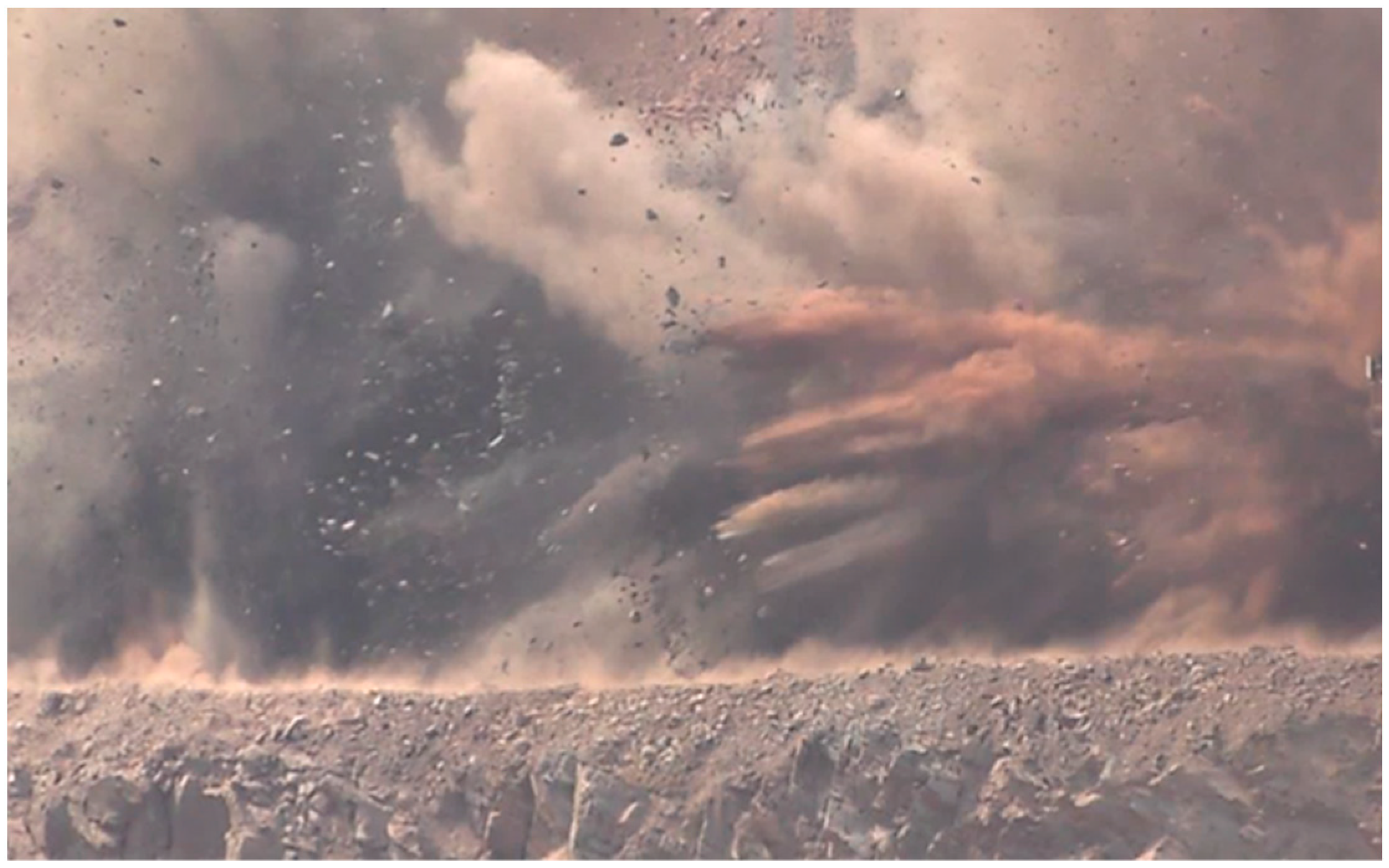
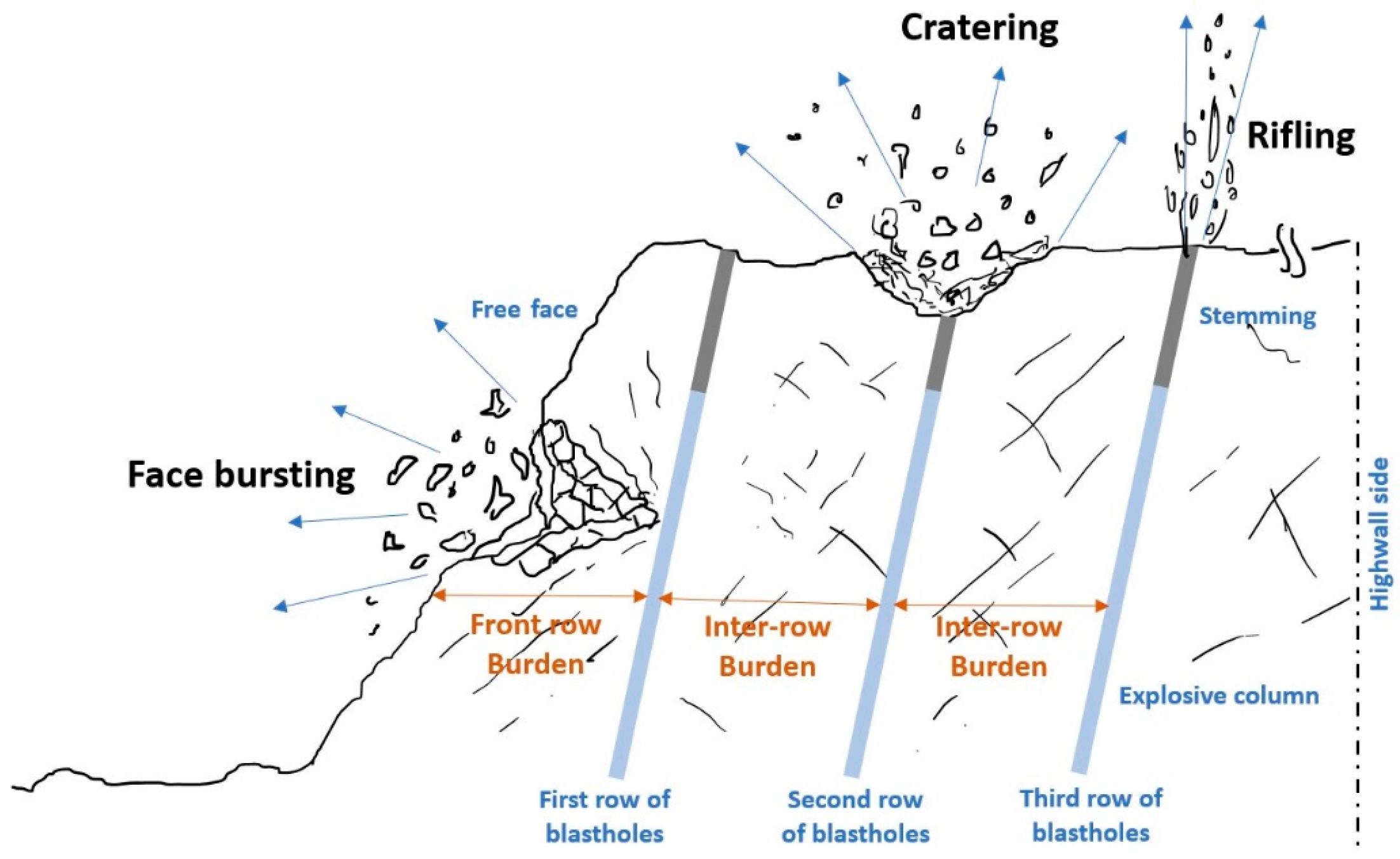

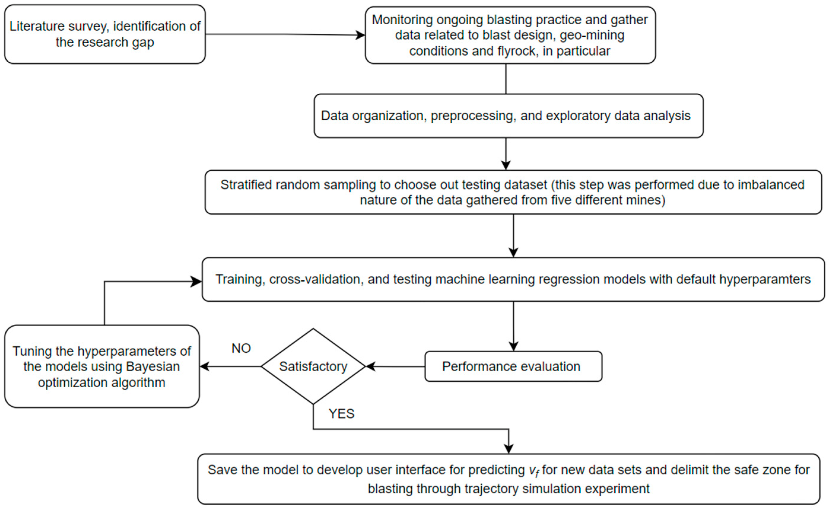

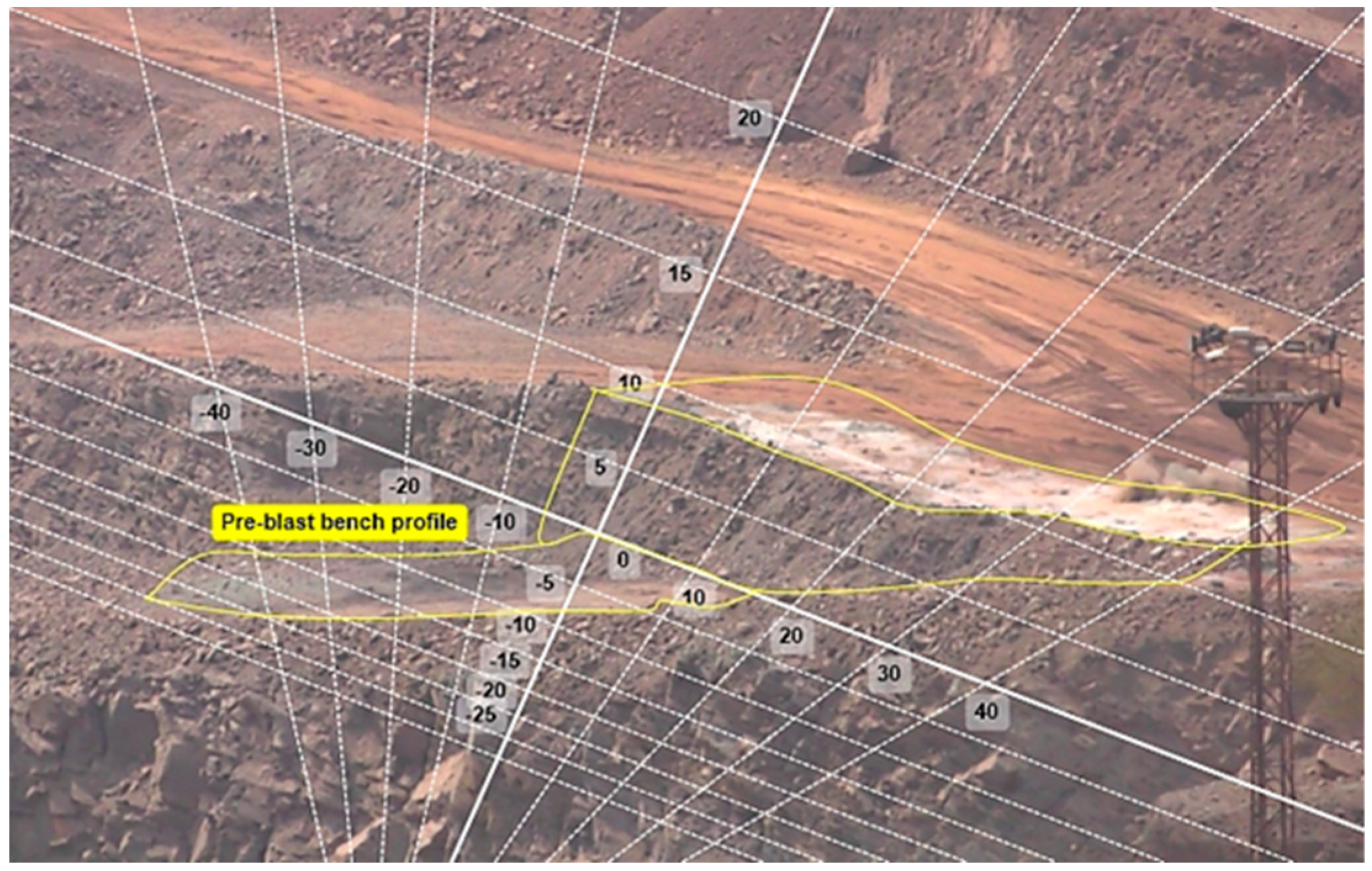
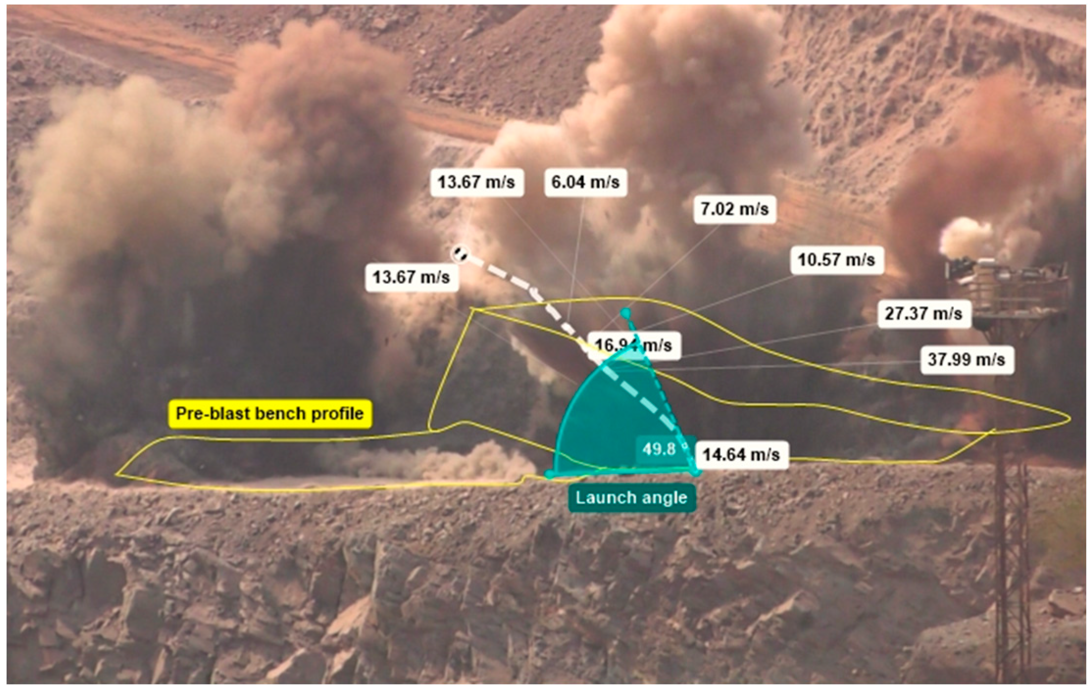

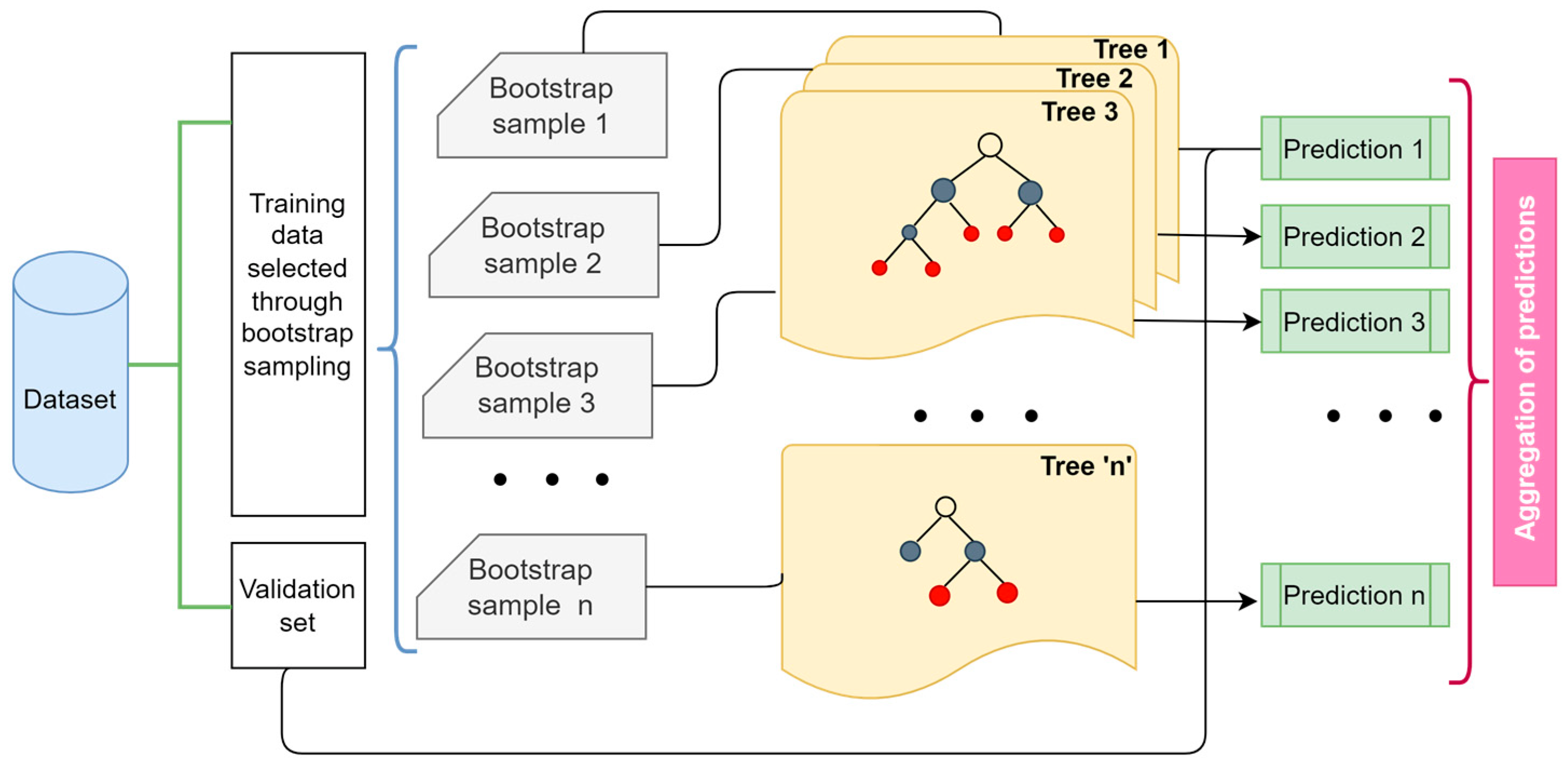
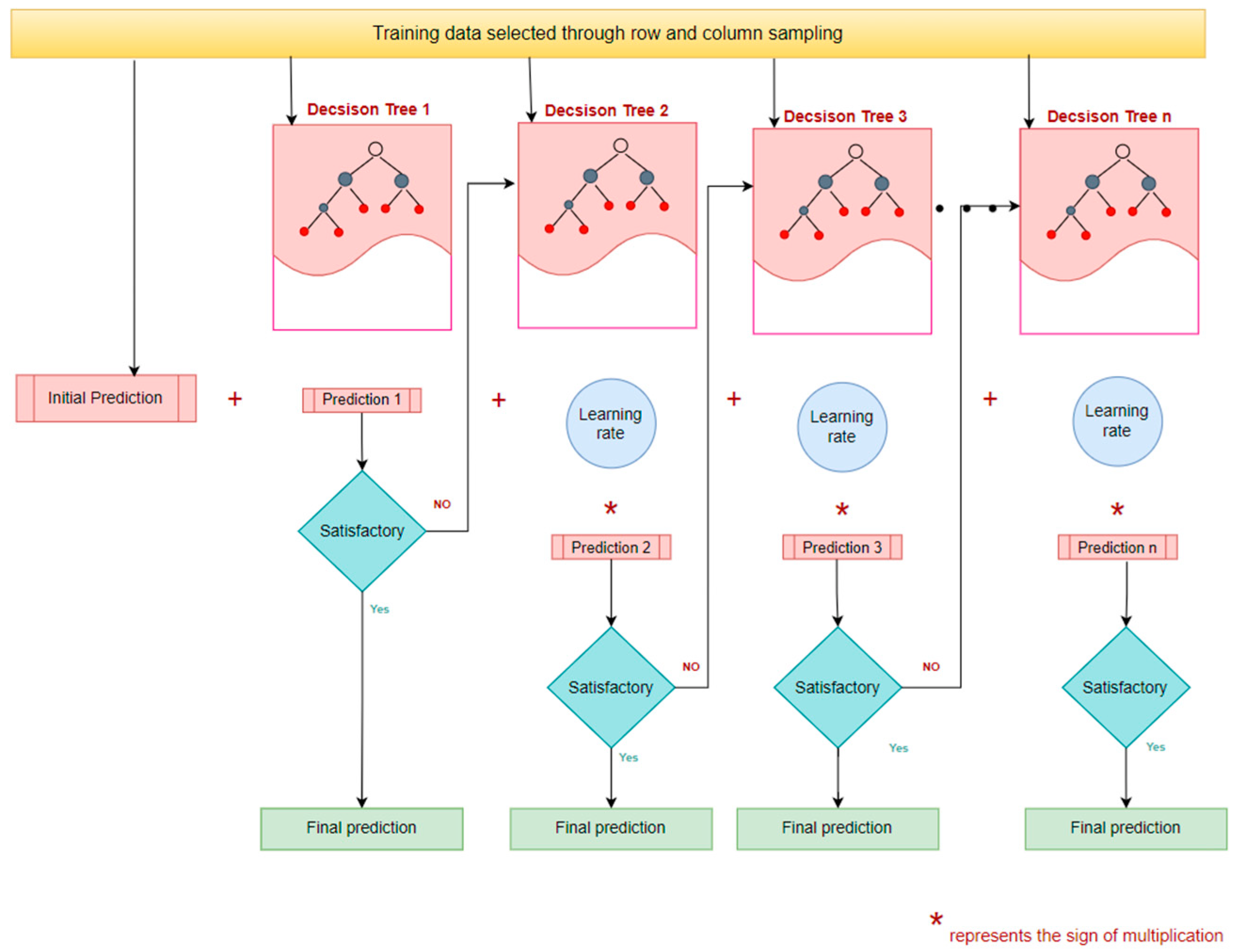
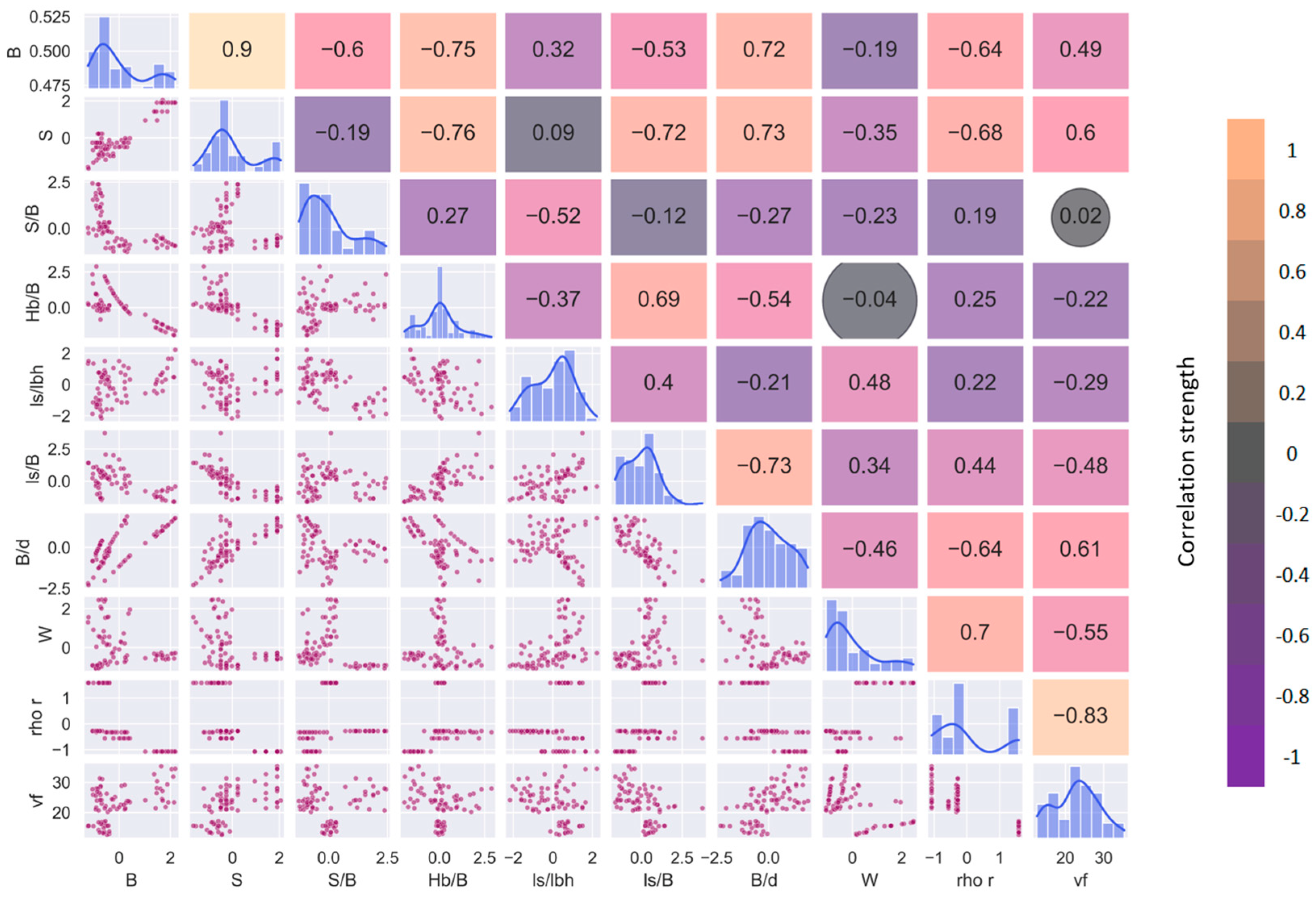


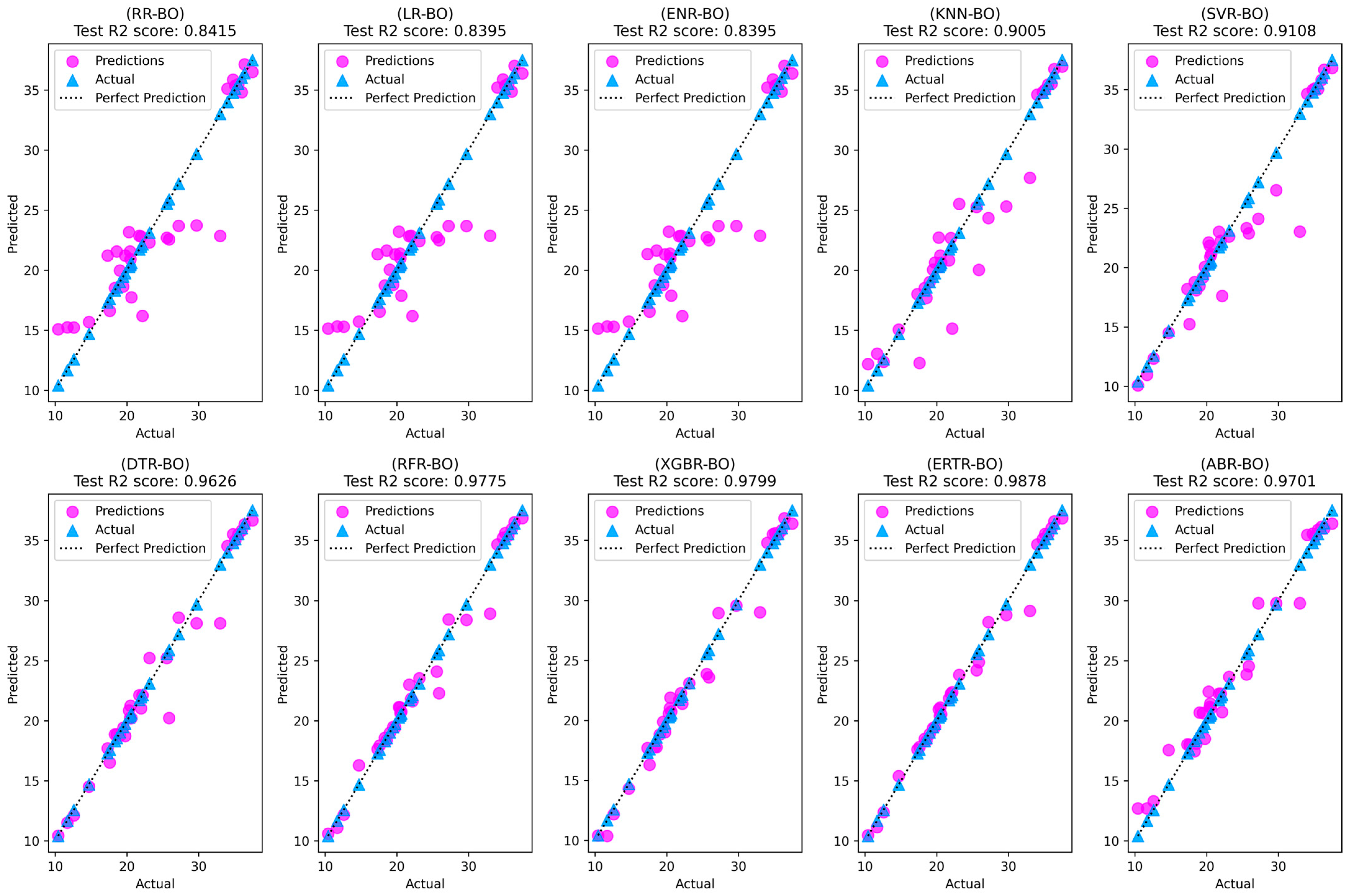
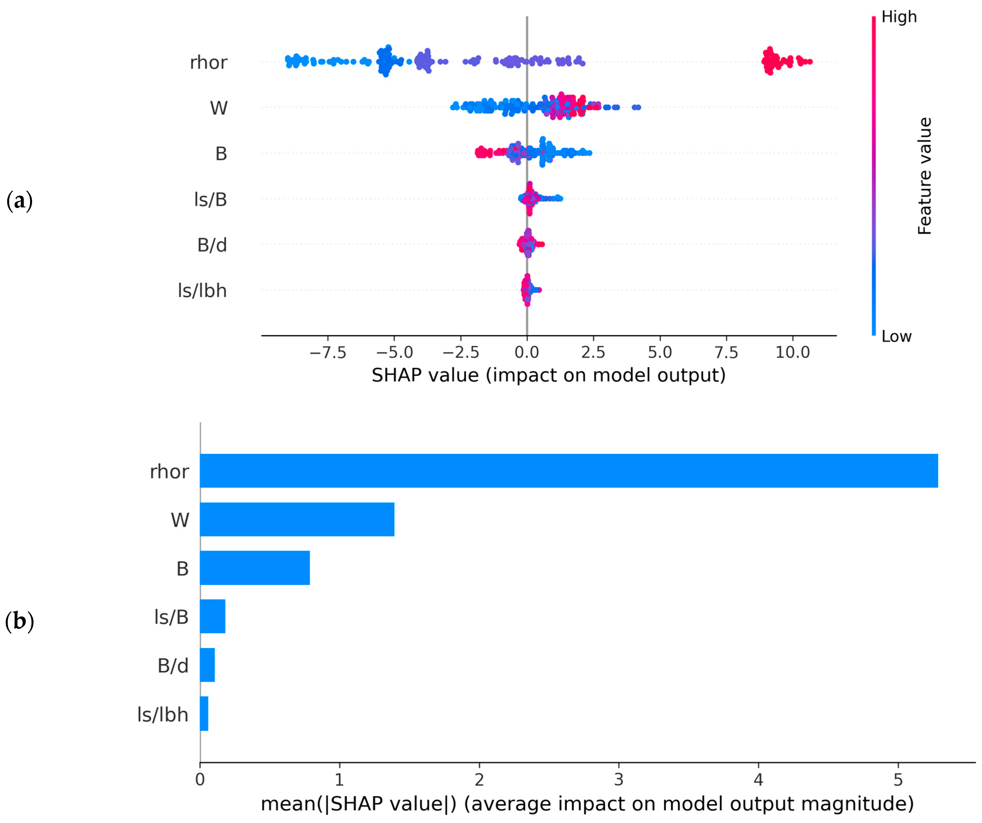

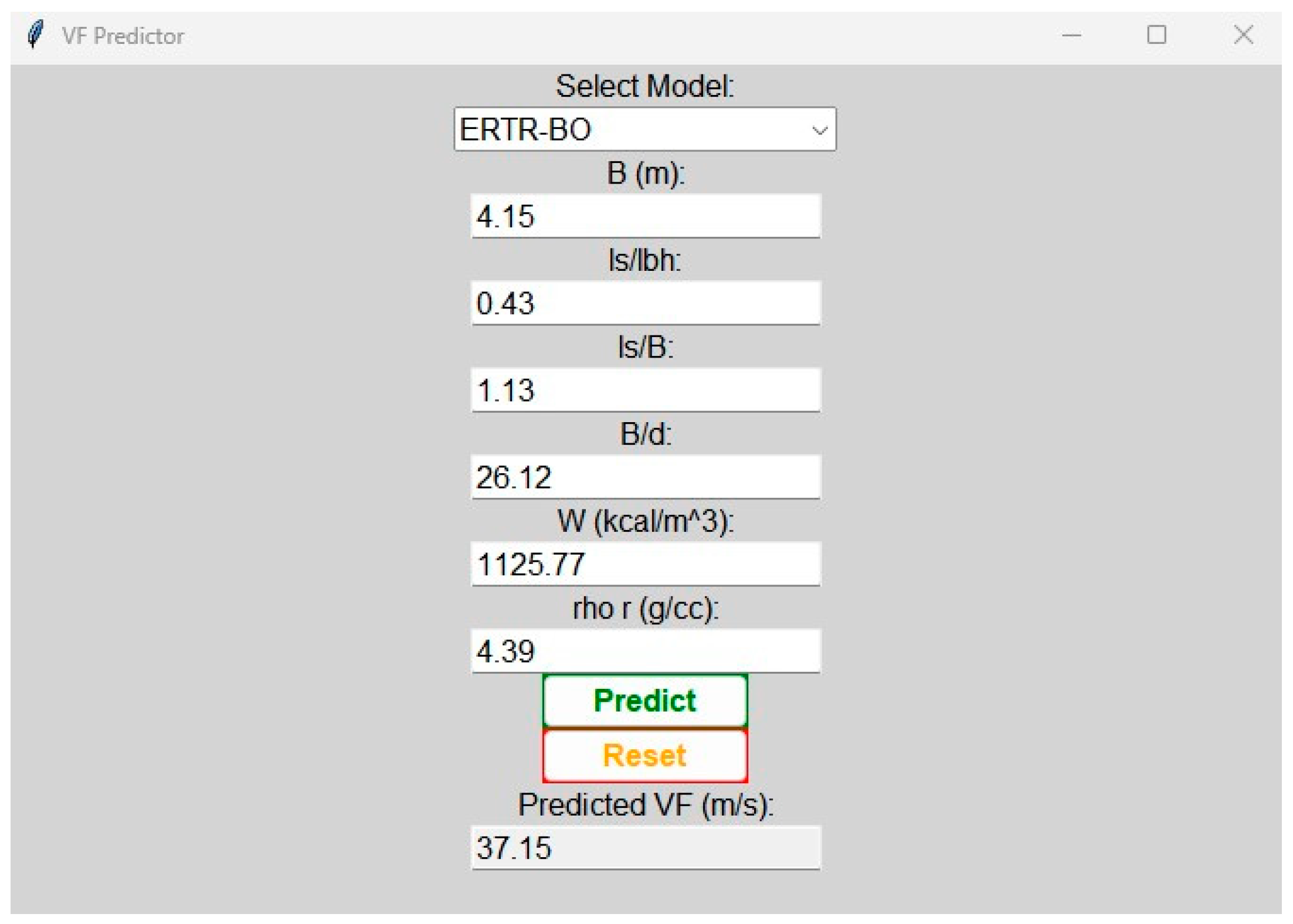
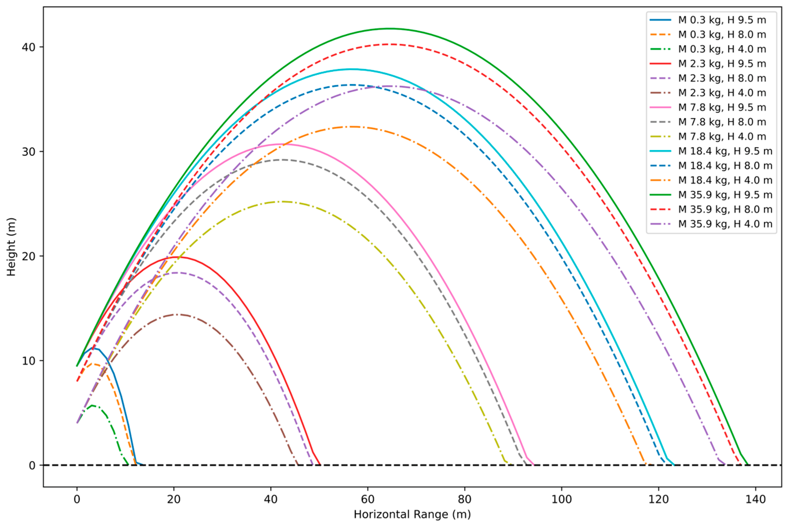
Disclaimer/Publisher’s Note: The statements, opinions and data contained in all publications are solely those of the individual author(s) and contributor(s) and not of MDPI and/or the editor(s). MDPI and/or the editor(s) disclaim responsibility for any injury to people or property resulting from any ideas, methods, instructions or products referred to in the content. |
© 2023 by the authors. Licensee MDPI, Basel, Switzerland. This article is an open access article distributed under the terms and conditions of the Creative Commons Attribution (CC BY) license (https://creativecommons.org/licenses/by/4.0/).