A Few-Shot Automatic Modulation Classification Method Based on Temporal Singular Spectrum Graph and Meta-Learning

Abstract

Deep learning-based Automatic Modulation Classification (AMC) has achieved excellent classification accuracy. However, most deep learning-based AMC methods have an inherent drawback. They exhibit a strong dependency on massive labeled samples, which is precisely difficult to obtain in real-world scenarios. This paper presents a few-shot AMC approach that integrates signal transformation and meta-learning. The former enhances class separability, while the latter addresses challenges posed by limited sample sizes. The results of simulation experiments conducted on the RadioML.2018.01a dataset demonstrate that the proposed technique achieves a classification accuracy of 74.21% when using one sample per class and increases to 82.27% when using five samples. The few-shot AMC efficacy of this proposed approach exhibits an outperformance over the classical deep learning methods.

1. Introduction

With the rapid development of modern communication technology, there has been an expanding trend in the types and complexity of modulation methods used in wireless communication [1]. Furthermore, the exponential growth in user demands and data volume continues to drive the increasing complexity of communication environments [2]. Consequently, the rapid and automated identification and classification of communication signals have become particularly crucial. AMC plays a key role in numerous civilian and military applications of wireless communication, including cognitive radio, electronic warfare, spectrum monitoring, surveillance analysis, and radio fault detection [3,4,5,6]. Serving as an intermediary between signal detection and demodulation, AMC greatly facilitates the effective classification of the modulation types. Thus, having a reliable and efficient AMC model is of paramount importance.

Traditional AMC methods can be categorized as decision theory-based and feature-based [7]. The former constructs a maximum likelihood function using statistical characteristics to determine modulation type through optimal decision thresholds. Methods like ALRT [8], GLRT [9], and HLRT [10] fall into this category. However, these methods require substantial prior knowledge and complex computations, posing challenges in non-cooperative communications. The latter identifies modulation type by comparing artificial features with theoretical values, requiring effective feature extraction techniques like constellation diagrams [11], fourth-order spectra [12], and cyclo-spectrograms [13]. While feature-based methods are more computationally efficient and require less prior knowledge, they have lower recognition performance in low SNR scenarios. Thus, extracting effective features remains crucial.

1.1. Motivations

In recent years, deep learning has made remarkable achievements in signal processing, particularly demonstrating excellent performance in AMC. O’Shea et al. [14] introduced a Convolutional Neural Network (CNN) model for AMC, which utilized temporal data for training and employed a softmax classifier to classify the extracted features. This approach surpassed the traditional methods that heavily rely on handcrafted features. Huynh-T et al. [15] proposed a new architecture with several specific convolutional blocks, achieving concurrent learning of spatial and temporal signal correlations. Perend et al. [16] implemented an improved CNN with additional layers to adapt estimated delays. In addition, other researchers not only focus on CNN structures, but also explore the advantages of Recurrent Neural Networks (RNNs) in AMC. In [17], a novel data-driven AMC model based on Long Short-Term Memory (LSTM) is proposed. This research demonstrated that LSTM-based models can accurately represent temporal sequences of different durations, which was highly valuable for modulation classification.

Nonetheless, the direct utilization of machine learning methods to accomplish AMC still presents two noteworthy challenges:

• When the raw and unprocessed signal is directly inputted, the model primarily conducts feature extraction on the original signal. However, the features derived through this approach often encapsulate only a fraction of the original signal’s characteristics, lacking a comprehensive and efficient capability for fulfilling the AMC task.
• Traditional machine learning relies heavily on data-driven pattern recognition and feature extraction, necessitating a substantial pool of well-labeled signal samples. Insufficient training samples can subsequently hamper the model’s generalization performance. In practical application, the intricate and varied nature of communication signals makes accumulating and labeling a substantial number of samples more complex. Frequently, only a limited number of samples are available, engendering a scenario where the model’s utilization of traditional machine learning-based methods might yield predictions with low confidence when it persists in conducting the AMC task under these constraints.

Consequently, our focus centers on the resolution of these two challenges.

1.2. Related Works

1.2.1. Signal Transformation

In the realm of direct machine learning-based AMC methods, the unprocessed signal sequence, when directly fed into the system, can be seen as a one-dimensional array housing minimal information. However, with the application of pre-processing techniques, the latent information embedded within can be more comprehensively revealed. In 1946, the Short-Time Fourier Transform (STFT) was introduced as the initial endeavor towards this goal. To tackle the aforementioned primary constraint, taking inspiration from STFT and subsequent research on two-dimensional representations of sequential signals, we have opted to address the prevailing issue by transforming the signal into a two-dimensional format.

Wang et al. suggested that encoding sequences into images allows machines to visually recognize, classify, and learn structures and patterns [18]. They utilize the Gramian Angular Field (GAF) to transform raw time-series data into a polar coordinate system. Additionally, they employ the Markov Transition Field (MTF) to compute the transition probabilities of a first-order Markov chain along the temporal axis. These pieces of information are regarded as the static and dynamic information of the time series. However, due to the inability of MTF to provide complete dynamic information and resulting in relatively lower classification accuracy compared to other newer methods, Hatami et al. proposed a representation method based on Recurrence Plots (RP) [19]. However, the simple CNN model they used led to imbalanced classification results on standard datasets. Reference [20] introduced a time-series image representation method called Motif Difference Field (MDF). By utilizing Gradient-weighted Class Activation Mapping (Grad-CAM) to identify important information within the sub-sequences and constructing MDF based on the differences between this information, the MDF is then classified using a Fully Convolutional Network (FCN) based on VGG16. Liu et al. [21] proposed a modulation recognition model based on multi-branch CNN. By leveraging prior knowledge of the signals and network topology, the time-domain waveforms of the signals were transformed into eye diagrams and constellation diagrams. The inherent advantages of CNNs in image recognition and classification were utilized to achieve modulation recognition. In [22], a deep learning-based method for MPSK signal modulation recognition was introduced. By extracting cyclic Poincaré maps of MPSK signals, two-dimensional feature information was obtained and fed into a CNN network for training, aiming to classify the modulation modes.

1.2.2. Meta-Learning

To address the constraint inherent in traditional machine learning, which demands an extensive array of labeled signal samples, we introduce the concept of meta-learning. Meta-learning, a learning paradigm inspired by biological systems, strives to transcend the limitations of conventional deep learning networks regarding their capacity for generalization and adaptability across diverse scenarios. The core idea involves improving learning algorithms or models by discerning relationships among interconnected tasks, mitigating challenges posed by limited data and subpar generalization in traditional deep learning. In typical machine learning, models are trained with abundant labeled data to learn associations between inputs and outputs. In contrast, meta-learning entails a training phase where models accumulate experience from diverse tasks. In the subsequent testing phase, models rapidly adapt to new tasks with limited labeled samples.

Tasks in meta-learning consist of a support set and a query set:

• The support set, a small example collection, trains the model on the same classes it will be tested on. The model derives insights from this set to update its parameters and apply them to the query set.
• The query set, used for evaluation, tests the model using knowledge acquired from the support set. It guides the model’s training process.

Furthermore, meta-learning often employs the N-way K-shot task setting. In each task, the model learns from N categories, each containing K samples in the support set.

Within the realm of deep learning tasks, meta-learning methods can be implemented through two primary approaches: metric-based and optimization-based. In metric-based meta-learning, the objective is to acquire an appropriate metric space for classification by comparing the distances between sample features. Vinyals et al. [23] proposed matching networks for one-shot learning. It utilizes an attention mechanism and matching process to classify query samples based on support set samples. Snell et al. [24] presented prototypical networks for few-shot learning. It learns prototype vectors for each class in the feature space and performs classification based on the distance between query samples and prototype vectors. Sung et al. [25] introduced relation networks for few-shot learning. It learns the relationship between query samples and support set samples through a sub-network and uses the learned representation to classify query samples. Conversely, optimization-based meta-learning aims to learn superior network initialization parameters by drawing insights from related tasks. Encountering new tasks, the network is fine-tuned with a small number of samples to achieve performance comparable to conventional deep learning models trained on extensive data. Finn et al. [26] proposed Model-Agnostic Meta-Learning (MAML) for fast adaptation of deep networks. It optimizes the initialization parameters through repeated adjustments on different tasks, enabling quick adaptation to new tasks. Reptile [27] is an iterative meta-learning algorithm that approximates the gradient descent process. It updates the model parameters multiple times on each task and performs a weighted average with the initial parameters to learn a model with good generalization. Rusu et al. [28] introduced LEO (Latent Embedding Optimization) as a meta-learning method. It learns a low-dimensional representation space where samples are mapped. It employs gradient descent to train the embedding network, enabling fast adaptation to new tasks using a few samples.

1.3. Contributions

As mentioned previously, the usage of meta-learning methods for model training is a proven idea to solve the problem of poor performance of AMC tasks under the few-shot condition to some extent. But the existing methods are mainly concentrated in the field of image classification, and the effect is not satisfactory when directly applied to the task of classification of modulated signals. For the characteristics of modulated signals, the existing meta-learning methods need to be appropriately modified and optimized to extract more effective prior knowledge. Targeting the above problems, this paper combines the method of image-based modulated signals with the meta-learning method, which provides a new way for the AMC task under few-shot conditions. The contributions of this paper are summarized in the following four points:

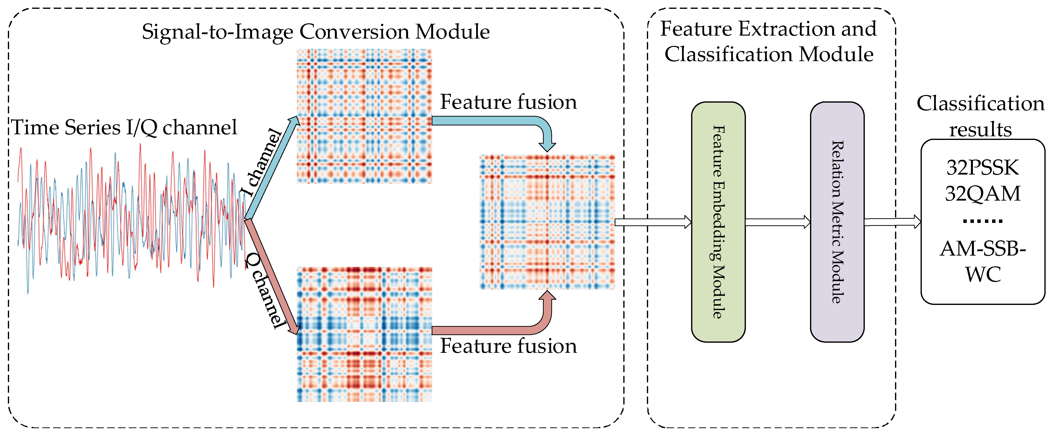
• We propose a novel approach that combines time-series signal visualization with meta-learning to tackle the small sample problem. We transform communication signals into images and employ a metric-based meta-learning method for feature extraction and classification.
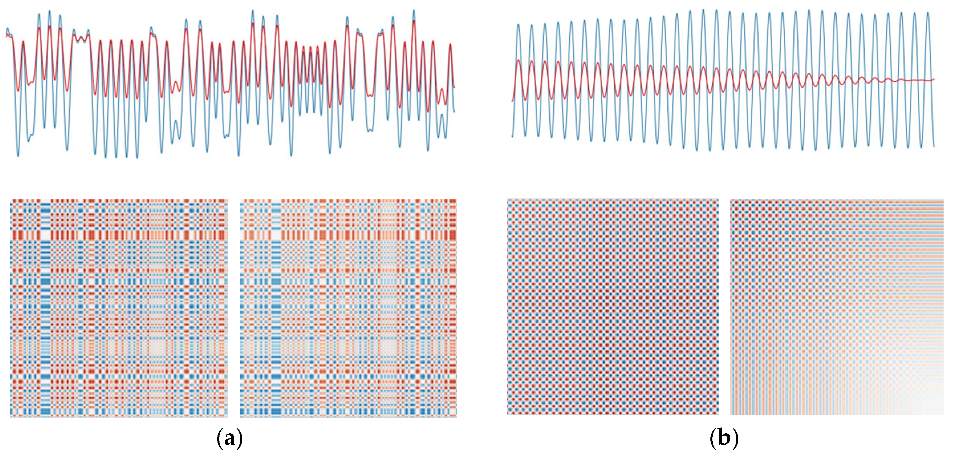
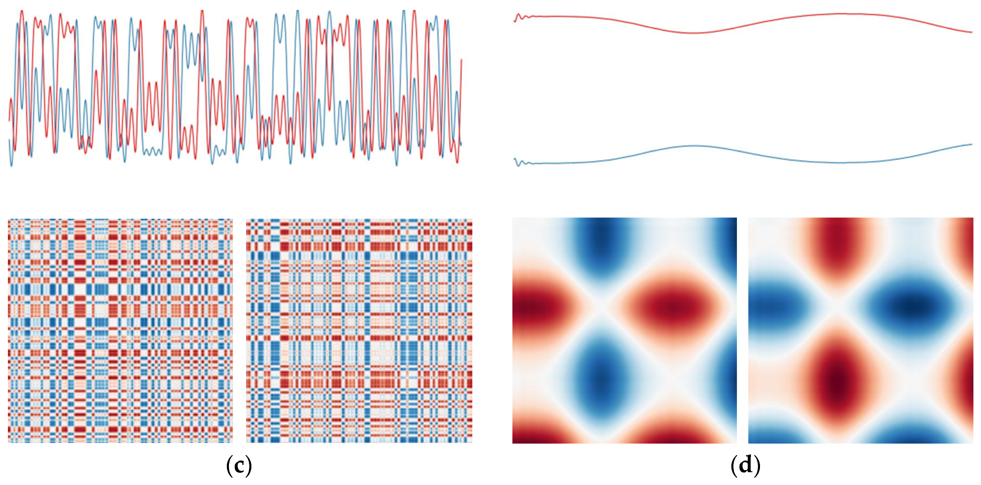
• In the signal representation stage, we employ Singular Spectrum Analysis (SSA) to reduce noise and eliminate redundant information in the signals. Subsequently, the signal sequences are transformed into two-dimensional images. This method enhances the exploration of signal content through signal decomposition and reconstruction. In contrast to traditional sequential signal processing methods that only extract features between adjacent time steps, this approach can capture the correlations between any two time points.
• In the classification stage, we adopt a metric-based relation network. The feature embedding module converts samples into high-dimensional feature representations Then, the relation metric module measures the distances between samples. Ultimately, this approach achieves AMC under the small sample condition.
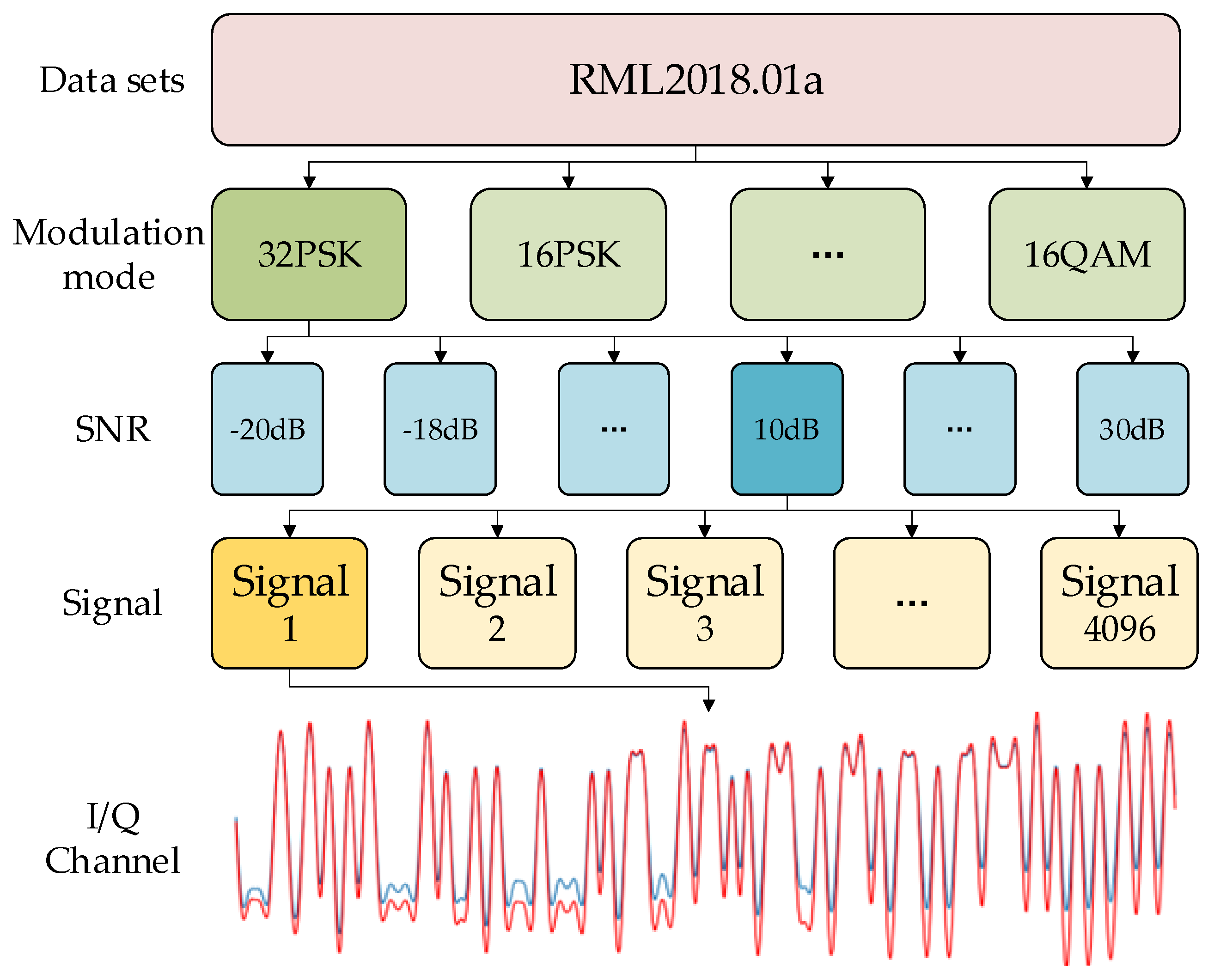
• We conduct simulations on the publicly available RadioML.2018.01a dataset to validate the advantages of the proposed method. Compared to the direct application of traditional machine learning methods for AMC, the method proposed in this paper attains higher recognition accuracy while employing a smaller number of samples. Furthermore, it demonstrates superior recognition capability when contrasted with the conventional approach of representing sequences.

1.4. Organization

The rest of this paper is organized as follows. Section 2 describes the signal model as well as the data processing methods we use and provides detailed information about the network. Section 3 reports the performance analysis of our approach and presents the results of comparative simulations. Section 4 concludes the paper.

2. Data Processing and Network Description

In this section, we illustrate our model in detail. As shown in Figure 1, the proposed algorithm is divided into two parts. In the first part, the time-series signals are processed using SSA, which effectively extracts the spectral features of the signals. By removing noise components, the impact of interference on the signal features is reduced, thereby improving the accuracy of the subsequent classification process. Then, the data from the I and Q channels are separately transformed into two-dimensional images. This is carried out to consider both the temporal and frequency domain information of the signals, enabling a more comprehensive representation of important signal features. Finally, at the end of the first part, the data from the I and Q channels are fused to obtain a more accurate and comprehensive feature representation.

In the second part, a meta-learning-based relation network is designed for the classification of unknown signals. In practical applications, there are usually only a limited number of samples available for training. Therefore, conventional deep learning methods that rely on large-sample training struggle to adapt to small-sample conditions. To overcome this problem, we introduce meta-learning. Meta-learning leverages shared knowledge and patterns learned from different tasks, enabling fast adaptation to new tasks even with limited samples. Firstly, the feature embedding module is used to extract features from the images obtained in the first part. Then, the relation metric module learns the similarity metric among the known modulation signal samples. Finally, the unknown signals are thoroughly classified.

2.1. Signal Model

In communication systems, signals are subject to various interferences such as channel fading, multipath interference, and noise during transmission. To accurately simulate the real communication environment, noise $n\left(t\right)$ is typically introduced into the communication model. The signal model is commonly represented as follows:

$$y\left(t\right)=x\left(t\right)+n\left(t\right),$$

(1)

where $y\left(t\right)$ represents the received complex envelope, $x\left(t\right)$ denotes the actual modulated signal, which is influenced by various unknown parameters, expressed as follows:

$$x\left(t,{\mathrm{u}}_i\right)=a{\sum }_{n=0}^{N-1} s_n^{k,i}{e}^{\mathrm{j}\left(\omega t+\theta \right)}{e}^{\mathrm{j}{\phi }_n}g\left(t\right),$$

(2)

where ${\mathrm{u}}_i$ represents the multidimensional parameter space of unknown quantities that affect the signal under the modulation mode $i$.

$${\mathrm{u}}_i=\left\{a,\theta ,\epsilon ,h\left(t\right),{\left\{{\phi }_n\right\}}_{n=0}^{N-1},{\left\{s^{k,i}\right\}}_{k=1}^{M_i},\omega \right\},$$

(3)

where $a$ represents the unknown signal amplitude, $\theta$ represents the carrier phase and phase offset caused by propagation, $\epsilon$ represents the time offset between the transmitter and receiver, $h\left(t\right)$ represents the channel impulse response, $\left\{{\phi }_n\right\}$ represents the phase offset parameters which are a set of continuous random variables, $\left\{s^{k,i}\right\}$ represents $K$ data symbols for the $i$-th modulation scheme, and $\omega$ represents the carrier frequency parameter.

2.2. Temporal Singular Spectrum Graph

This paper proposes an improved transformation method for visualizing sequential data called Temporal Singular Spectrum Graph (TSSG). The specific implementation is as follows:

• Preprocessing. For a sequence $S=\{s_1,s_2,\dots ,s_N\}$ with length $N$, the sequence is first standardized by the following formula:

$$x_i=\frac{\left(s_i-\mu \right)}{ \sigma },$$

(4)

where $\mu$ represents the mean of the sequence, and $\sigma$ represents the standard deviation of the sequence. In this method, for each value in the sequence data, it is subtracted by the mean of the sequence and then divided by the standard deviation of the sequence. This transformation ensures that each value in the sequence becomes a deviation from the mean, relative to the standard deviation of the sequence. It normalizes the variables to the same scale, making them comparable in numerical terms and improving the accuracy of subsequent classifiers. As a result, a new sequence $X=(x_1, x_2,\dots ,x_n)$ is obtained, with a mean of 0 and a standard deviation of 1.

• Constructing trajectory matrix. For the given sequence, a sliding window is defined with a window length of $L$, satisfying $L\le \frac{T}{2}$. Simultaneously, $K$ is defined as $K=N-L+1$, which is used to construct the trajectory matrix. The first column of the matrix represents $y_1$ to $y_L$, the second column represents $y_2$ to $y_{L+1}$, etc., until the $L$-th column represents $y_K$ to $y_N$. The resulting trajectory matrix is as follows:

$$\begin{array}{ll}\mathbf{Y}& ={\left(x_{ij}\right)}_{i,j=1}^{L,K}\\ & =\left(\begin{array}{ccccc}{y}_1& y_2& y_3& \dots & y_K\\ y_2& y_3& y_4& \dots & y_{K+1}\\ ⋮& ⋮& ⋮& \ddots & ⋮\\ y_L& y_{L+1}& y_{L+2}& \dots & y_N\end{array}\right)\end{array},$$

(5)

The matrix $\mathbf{Y}$ is a Hankel matrix, where $y_{i,j}=y_{i-1,j+1}$.

Singular Value Decomposition (SVD). The matrix $\mathbf{Y}$ is subjected to Singular Value Decomposition, resulting in matrices $\mathbf{U}$,$\mathbf{V},\mathsf{\Sigma }$, where $\mathbf{U}$ and $\mathbf{V}$ are orthogonal matrices, and $\mathsf{\Sigma }$ is the singular value matrix. The singular values are denoted as $\sigma$ and are sorted in descending order: ${\mathsf{\sigma }}_1\ge {\mathsf{\sigma }}_2\ge \dots \ge {\mathsf{\sigma }}_L\ge 0$. The contribution value $C_i$ is defined as $C_i=\frac{{\mathsf{\sigma }}_{\mathrm{i}}}{{\sum }_1^L\mathsf{\sigma }}$, representing the contribution of the i-th singular value. A larger sum of contribution values for the top $k$ singular values indicates that the reconstructed sequence can better represent the original sequence.

• Matrix Reconstruction: Based on the magnitude of the singular values $\mathsf{\sigma }$, the number of principal components $k$ in the sequence is determined. The left singular vectors corresponding to the $k$ largest singular values (i.e., the first $k$ columns of matrix $\mathbf{U}$) are selected to construct matrix ${\mathbf{U}}_{\mathbf{k}}$. Simultaneously, the right singular vectors corresponding to the $k$ largest singular values (i.e., the first $k$ columns of matrix $\mathbf{V}$) are selected to construct matrix ${\mathbf{V}}_{\mathbf{k}}$. Then, the reconstruction matrix ${\mathbf{X}}_{\mathbf{R}}$ is obtained.

$$\begin{array}{ll}{\mathbf{X}}_{\mathbf{R}}& =U_k{{\Sigma }_{k}V}_k^T\\ & ={\sum }_{i=1}^k{\mathsf{\sigma }}_i{u}_i{v}_i^T\\ & ={\mathbf{X}}_1+{\mathbf{X}}_2+\cdots +{\mathbf{X}}_{\mathbf{k}}\end{array},$$

(6)

where ${\mathbf{X}}_1$, ${\mathbf{X}}_2$, …, ${\mathbf{X}}_{\mathbf{k}}$ represent the reconstructed submatrices.

• Sequence Reconstruction. The reconstructed sequence $R$ is obtained by performing anti-diagonal averaging reconstruction on the reconstructed submatrix ${\mathit{X}}_{\mathit{k}}$. Here, $1⩽i⩽L,1⩽j⩽K$. Let $L^{\ast }=\mathrm{m}\mathrm{i}\mathrm{n}(L,K)$ and $K^{\ast }=\mathrm{m}\mathrm{a}\mathrm{x}(L,K)$. The reconstruction of sequence $R$ can be calculated using the following formula:

$$R=\left\{\begin{array}{ll}\frac{1}{k}{\sum }_{m=1}^k x_{m,k-m+1}^{ }& 1⩽k<L^{\ast }\\ \frac{1}{L^{\ast }}{\sum }_{m=1}^{L^{\ast }} x_{m,k-m+1}^{ }& L^{\ast }⩽k⩽K^{\ast }\\ \frac{1}{N-k+1}{\sum }_{m=k-K^{\ast }+1}^{N-K^{\ast }+1} x_{m,k-m+1}^{ }& K^{\ast }<k⩽N\end{array}\right.,$$

(7)

• Visualization. The reconstructed sequence $R$ is copied $k$ times along the column direction, and then the transpose of $R$ is obtained as a $k\times 1$ column vector. This process generates two matrices: one where each row is equal to $R$, and another where each column is equal to $R$. By subtracting these two matrices, a $k\times k$ matrix $\mathbf{M}$ is obtained, representing the Euclidean distance between every pair of points. Similar to a recursive graph, each row and column of matrix $\mathbf{M}$ contains information about the entire sequence. Finally, the matrix $\mathbf{M}$ is transformed into a grayscale image using max-min normalization, resulting in the desired image.

Figure 2 illustrates the transformed images of signal sequences from the RadioML2018.01a dataset, from which we can see that TSSG can effectively capture the information of the original signals. The figure showcases four different signals (32PSK, QPSK, OOK, 64QAM) represented as TSSG, generated under 30 dB SNR. Each signal is divided into the I and Q components. In the waveform plots, the I component is depicted in blue, while the Q component is shown in red. To better visualize the characteristics of these signals, each group of images consists of the TSSG of the I component on the left and the TSSG of the Q component on the right.

From Figure 2, we can clearly observe the characteristics of the original signals. Rapidly changing signals in the waveform plot are represented by abrupt color transitions, while smoothly changing signals appear as regions of solid color. Low-frequency signals exhibit smoother patterns, whereas high-frequency signals display more pronounced variations, facilitating the differentiation of different modulation types. The I and Q components of the 32PSK signal exhibit almost identical variations, but the amplitude of the Q component is smaller than that of the I component, resulting in nearly consistent patterns in the transformed images, albeit with lighter colors. The QPSK signal demonstrates intense variations, thus appearing as a dense grid of points in the image, with the Q component gradually decreasing in amplitude, leading to a transparent effect in the bottom right corner of the image. The OOK signal exhibits rapid and chaotic changes, which are reflected in its transformed image. The 64QAM signal, both in the I and Q components, undergoes smooth variations, resulting in large areas of solid color in the transformed image. Moreover, the I and Q components exhibit opposite trends, resulting in identical shapes but contrasting colors.

2.3. Relation Network

After transforming the signal samples into two-dimensional images, this paper employs a meta-learning framework based on a relational network to classify these preprocessed signal images.

2.3.1. Network Structure

The main distinction of the relation network from other metric learning models lies in its ability to compute similarity scores between each test sample and each class by learning an adjustable similarity metric. This enables more efficient and accurate classification. The relation network consists of two core components: the feature embedding module and the relation metric module.

The feature embedding module is responsible for mapping signal samples into a feature metric space. This mapping process aids in extracting key features from TSSG, providing richer information for subsequent relation metric computation. Then, the relation network concatenates the extracted feature vectors of the test signal sample with the support set. Subsequently, the relation metric module computes similarity scores between the test signal and each class’s signal from the support set. Based on these similarity scores, the relation network can classify the test signal sample.

2.3.2. Feature Embedding Module

The feature embedding module, as previously mentioned, plays a crucial role in the transformation of input images. In the context of few-shot learning tasks, our objective is to transform the images from the support set and query set into vector representations for similarity computation and pattern recognition.

In this paper, we adopt a CNN that incorporates the Squeeze-and-Excitation Network (SENet) [29] as the feature extractor to capture key features in the images. CNNs possess the characteristics of local perception and weight sharing, enabling effective extraction of both local and global information from the images. The model aims to enhance the expressive power of the network by adaptively learning the importance of feature channels. Its core idea lies in the introduction of a mechanism called “Squeeze-and-Excitation”, which automatically learns the weights for each channel to amplify more important feature channels and attenuate relatively less important ones. The SENet structure consists of two main parts: the Squeeze part and the Excitation part.

• The Squeeze part reduces the dimensionality of the input feature maps through global average pooling, transforming them into a fixed-size vector. This vector can be regarded as the global statistical information of the entire feature map, encompassing the overall characteristics of each channel. Specifically, for an input feature map with a size of H × W × C (height × width × number of channels), the Squeeze operation produces a feature map of size 1 × 1 × C.
• The Excitation part is the core component of SENet, which processes the output of the Squeeze operation through a fully connected layer and an activation function. The output size of the fully connected layer is C × r (where r is a tunable scaling factor typically chosen to be small), followed by a ReLU activation function for non-linear mapping. Finally, another fully connected layer restores the size of the feature map to C. This process can be seen as a re-calibration of the feature channels, allowing for the learning of weights for each channel.

In SENet, the output of the Excitation part is normalized using a sigmoid function to ensure that the weights for each channel fall within the range of 0 to 1. Ultimately, the normalized weights are applied to each channel of the input feature map, achieving channel-wise adaptive weighting. By introducing the SENet module, the network can adaptively learn the importance of each channel and its importance in different spatial locations. This enables SENet to effectively leverage the relationships among channels and the diversity of features, thereby improving the performance of image classification tasks.

In the feature extraction process, multiple layers of convolutional layers and activation functions are used to enhance the expressive power and non-linear fitting capability of the model. A global pooling layer and a fully connected layer are introduced at the output end of the CNN to map the extracted high-dimensional features to a low-dimensional space. Max pooling effectively reduces the feature dimensionality, reducing computational complexity while preserving global information. The fully connected layer is responsible for linearly transforming the pooled features, generating the final low-dimensional vector representation. The network structure of the feature embedding module used in this paper is shown in

Table 1. Structure of the feature embedding module.

Layer	Type	Output Shape
Input		3 × 84 × 84
1	Conv2d	64 × 82 × 82
	BatchNorm2d	64 × 82 × 82
	ReLU	64 × 82 × 82
	MaxPool2d	64 × 41 × 41
	SEBlock	64 × 41 × 41
2	Conv2d	64 × 39 × 39
	BatchNorm2d	64 × 39 × 39
	ReLU	64 × 39 × 39
	MaxPool2d	64 × 19 × 19
3	SEBlock	64 × 19 × 19
	Conv2d	64 × 19 × 19
	BatchNorm2d	64 × 19 × 19
	ReLU	64 × 19 × 19
	SEBlock	64 × 19 × 19
4	Conv2d	64 × 19 × 19
	BatchNorm2d	64 × 19 × 19
	ReLU	64 × 19 × 19
	SEBlock	64 × 19 × 19

.

2.3.3. Relation Metric Module

The relation metric module is responsible for computing similarity scores between the test samples and each class. It consists of multiple convolutional and pooling layers, which effectively learn the similarity and dissimilarity features among different classes. By adaptively adjusting the similarity and dissimilarity between classes, the relation metric module can better adapt to different datasets and task requirements. The specific network structure is shown in

Table 2. Structure of the relation metric module.

Layer	Type	Output Shape
Input		128 × 19 × 19
1	Conv2d	64 × 17 × 17
	BatchNorm2d	64 × 17 × 17
	ReLU	64 × 17 × 17
	MaxPool2d	64 × 8 × 8
2	Conv2d	64 × 6 × 6
	BatchNorm2d	64 × 6 × 6
	ReLU	64 × 6 × 6
	MaxPool2d	64 × 3 × 3
3	Linear	8
4	Linear	1

.

The output of the relation metric module is a similarity score, which represents the similarity between the test sample and its corresponding class. By sorting the scores, the most similar class to the test sample can be identified, thus achieving the classification task.

3. Simulation Experiments and Analysis

3.1. Simulation Experiment

This paper utilized the publicly available RadioML dataset provided by DeepSig Inc., Arlington, VA, USA, specifically version RadioML2018.01a. The dataset consists of 24 different types of digital and analog modulation signals, including OOK, 8ASK, QPSK, 16PSK, 16APSK, 64APSK, 16QAM, 64QAM, 256QAM, AM-SSB-SC, 128QAM, AM-SSB-WC, FM, OQPSK, GMSK, 128APSK, BPSK, 4ASK, 8PSK, 32PSK, 32APSK, 32QAM, AM-DSB-SC, and AM-DSB-WC. The dataset covers a SNR ratio range of −20 to 30 dB. Each signal in the dataset contains both the in-phase I and quadrature Q components, with a length of 1024. The specific structure of the dataset is shown in Figure 3.

In order to ensure the representativeness of experimental results, experiments were conducted to divide the dataset of 24 different signal categories into training and testing sets using a ratio of 17:7. The dataset was partitioned randomly, taking into account various modulation schemes. Moreover, due to the inherent characteristics of meta-learning, the labels assigned to the training and testing sets were entirely separate. Specific details regarding the dataset partitioning are provided in

Table 3. Dataset partitioning for experiments in this paper.

	Modulation Type
Train Set	16APSK FM GMSK 32APSK OQPSK 8PSK AM-SSB-SC 4ASK 64QAM 16PSK 64APSK 128QAM AM-SDB-SC AM-DSB-WC 256QAM OOK 16QAM
Test Set	32PSK 32QAM 8ASK BPSK 128APSK QPSK AM-SSB-WC

.

The simulation experiments were conducted with SNRs ranging from −10 dB to 18 dB in steps of 2 dB, resulting in a total of 15 different SNR values. For each SNR, 100 random samples were extracted for each signal class. The extracted signal features using TSSG were then fed into the relation metric network for classification training.

The experiments in this paper were based on the N-way K-shot setting. In this setting, N represents the number of classes and K represents the number of samples per class. In the meta-learning network, the extracted features had a dimensionality of 64, the learning rate was set to 0.001, and the Adam [30] optimization algorithm was employed.

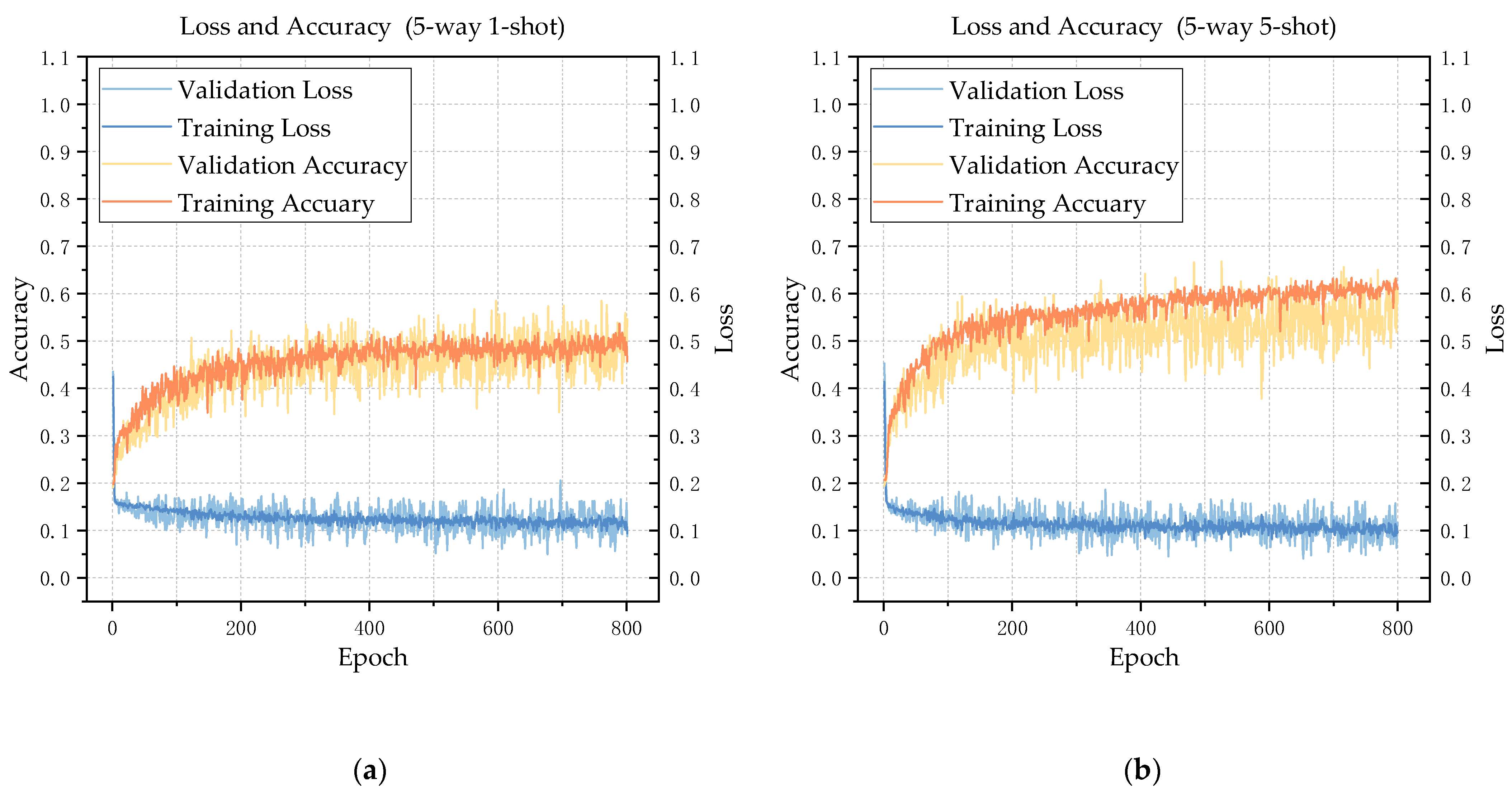
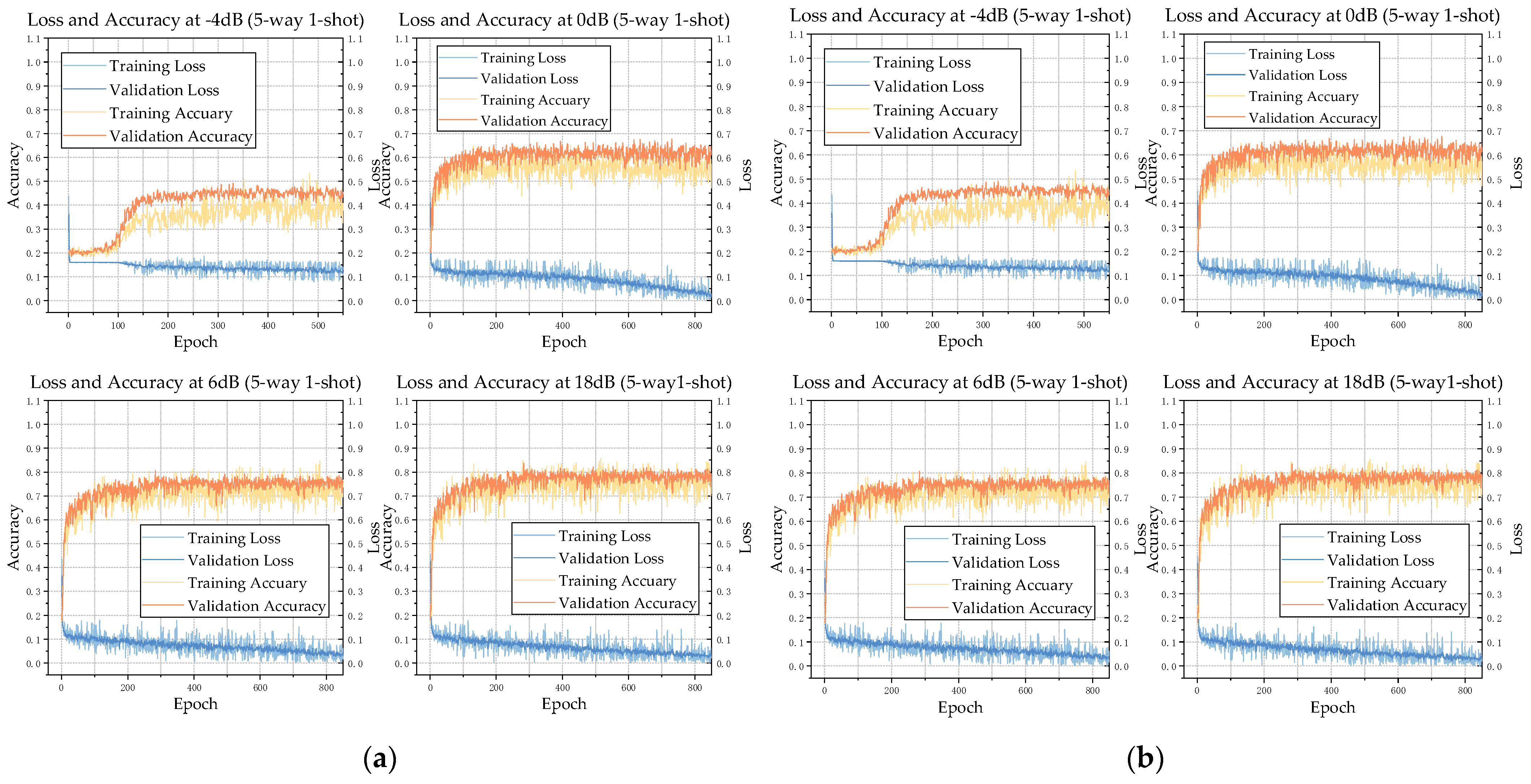
3.2. Model Performance Analysis

In this section, we focus on analyzing the loss and accuracy of the model under the two classic conditions of 5-way 5-shot and 5-way 1-shot. Due to the smaller dataset in meta-learning compared to traditional machine learning methods, the loss and accuracy exhibit more pronounced fluctuations.

As shown in Figure 4, regardless of the conditions of 5-way 5-shot and 5-way 1-shot, the loss rapidly decreases and converges at the beginning. The loss measures the gap between the model’s predicted results and the actual results, and its decrease indicates a gradual improvement in the model’s performance. When the loss converges, it means that the model has found a set of parameters that minimizes the loss function, resulting in optimal model performance. At the same time, the accuracy continuously increases, indicating that the model is learning and acquiring knowledge from the data. As it progresses, the model’s predictions for the data become increasingly accurate. By comparing the results, it is evident that 5-way 5-shot outperforms 5-way 1-shot. Compared to using only one signal sample to represent each category in 5-way 1-shot, 5-way 5-shot provides more information, enabling the model to converge faster and significantly improve accuracy. This allows the model to better understand and differentiate the differences between different modulation schemes.

To further investigate the performance of the model, we conduct separate tests on four representative signal-to-noise ratios (SNRs): −4 dB, 0 dB, 6 dB, and 18 dB. Specifically, we focus on analyzing the loss and accuracy under the 5-way 5-shot and 5-way 1-shot conditions for each SNR. For these individual tests at different SNRs, we delete the weight files and randomly initialize the model parameters. Additionally, since the accuracy in the graph is calculated on the set, the maximum accuracy reaches 1, which is different from the accuracy during testing. The experimental results are shown in Figure 5.

Under −4 dB SNR, the signal energy is relatively small compared to the noise energy, resulting in a mixture of the signal and noise that is difficult to distinguish. As a result, the model is initially trapped in a local optimum, leading to little change in the loss and accuracy for a while. However, the Adam optimizer, which employs adaptive learning rates and incorporates the concept of momentum, dynamically adjusts each parameter and helps escape local optima. In the case of 5-way 5-shot, the loss starts to decrease, and the accuracy begins to rise, eventually reaching a lower loss value and a higher level of accuracy. This indicates that the model achieves good performance under −4 dB SNR. In the case of 5-way 1-shot, there is greater fluctuation in the loss and accuracy, and the convergence speed is relatively slower. It takes more epochs to escape from the local optimum, but the model is still able to continue converging. In the case of 5-way 5-shot, there is a noticeable improvement in convergence speed.

Under 0 dB SNR, the distinction between the signal and noise is relatively improved compared to −4 dB but still poses certain challenges. In this scenario, the loss and accuracy exhibit noticeable fluctuations. However, as it progresses, the convergence speed gradually accelerates, and the accuracy improves to some extent. Under the 5-way 5-shot condition, the loss quickly converges to a small value, and the accuracy simultaneously improves at the same time, with smoother fluctuations in both metrics. This indicates that the model still possesses some recognition capability under 0 dB SNR, although its performance may not be as strong as in higher SNR conditions.

Under 6 dB SNR, the convergence speed further improves, with the loss decreasing at a faster rate and stabilizing more quickly. This indicates that in higher SNR conditions, the model can learn effective features more rapidly, thereby enhancing its classification performance. Under both the 5-way 1-shot and 5-way 5-shot conditions, the model exhibits improved convergence speed and accuracy. However, the performance of the 5-way 5-shot setup is relatively superior, possibly since it utilizes more samples during each iteration, allowing the model to capture the differences between categories more effectively.

Under 18 dB SNR, the energy of the signal is relatively larger compared to the noise, resulting in a clearer distinction between the signal and noise. Consequently, the model can more accurately extract the signal’s features and identify the modulation types. Whether under the 5-way 1-shot or 5-way 5-shot conditions, the loss rapidly decreases, and the convergence speed is significantly faster than that observed at −4 dB and 0 dB. Additionally, the accuracy reaches a higher level within a short time and exhibits less fluctuation, indicating improved stability of the model at higher SNR. Furthermore, due to the clearer distinction between the signal and noise, the fluctuations in loss and accuracy become smoother, indicating increased stability of the model in this scenario.

The examination of the four subplots in each graph, organized according to SNR, highlights a noticeable trend. The model’s performance exhibits enhanced robustness with varying SNR levels. This phenomenon is attributable to SNR, which quantifies the proportion between signal and noise. A higher SNR denotes a more pronounced signal in relation to noise, whereas a lower SNR indicates a relatively stronger noise presence. In conditions of elevated SNR, signal degradation is minimal, and noise’s impact on the signal is limited. This prominence accentuates the manifestation of modulation pattern characteristics, thereby offering an amplified dataset for analysis during recognition. This reduction in susceptibility to noise interference ultimately stabilizes the model’s decision boundaries, facilitating clearer differentiation between distinct modulation patterns and augmenting recognition accuracy. Conversely, under lower SNR, the signal may be engulfed by noise, obscuring its features and providing unreliable data for analysis and learning. This hinders precise identification and separation, complicating pattern discrimination. It is noteworthy that the performance enhancement between 18 dB SNR and 6 dB SNR is marginal. At 6 dB SNR, the model has already garnered adequate information for proficiently classifying signal modulation patterns.

Furthermore, a juxtaposition of the two plots on the left and right unveils that, in terms of convergence speed and final accuracy post-convergence, the 5-way 5-shot condition generally outperforms the 5-way 1-shot counterpart. This difference emanates from the fact that the 5-way 5-shot scenario incorporates five samples per category, whereas the 5-way 1-shot condition encompasses merely one sample per category. This disparity stems from the understanding that an augmented pool of training samples typically aids the model in superiorly capturing features and patterns. The 5-way 5-shot condition presents a more substantial training dataset, facilitating more precise feature comprehension within each category. This, in turn, enhances the model’s adaptability to new tasks. As the model encounters novel tasks, it proficiently amalgamates knowledge accumulated from multiple tasks, thereby enabling improved distinction among diverse categories within new tasks.

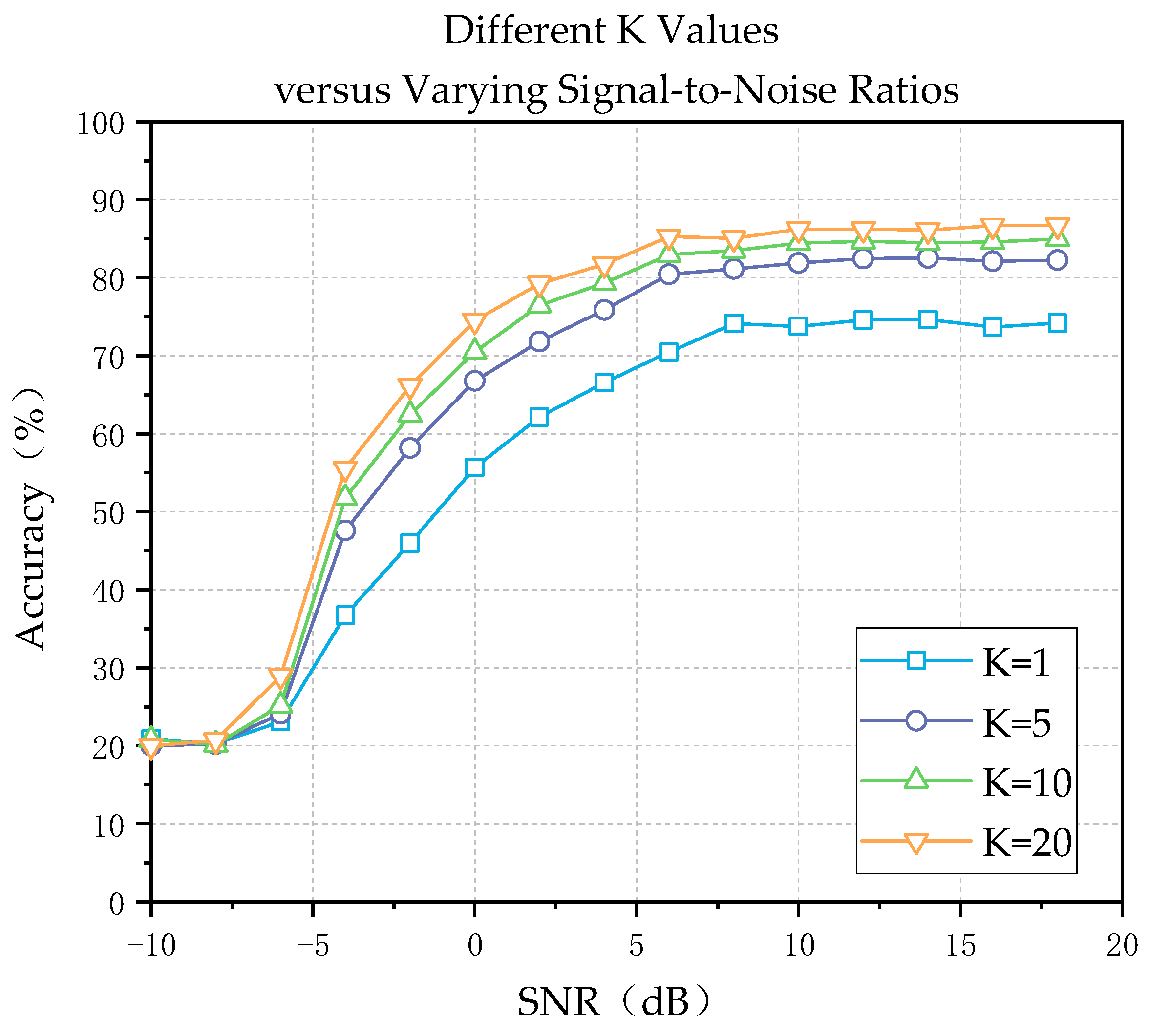
3.3. Performance Comparison with Different Values of K

In this section, we explore how the classification performance is affected by the number of samples in the support set (K) under the 5-way K-shot condition. To mitigate the influence of random factors, we consider four different values of K: 1, 5, 10, and 20. For each value of K, multiple experiments are conducted, and the average recognition rate is calculated. The experimental results are shown in Figure 6.

From Figure 6, we observe that when K = 1, the model achieves a recognition accuracy of 75.88% at 18 dB. This indicates that the proposed algorithm performs well even with only one training sample. When K = 5, the model achieves a recognition accuracy of 83.95%, which is an improvement of 8.07% compared to the case when K = 1. As the value of K increases, the average recognition rate of the model continues to improve. At 18 dB, with K = 10 and K = 20, the model achieves recognition accuracies of 86.16% and 88.30%, respectively. By increasing the value of K, we allow the model to learn the differences between classes from a larger sample pool, thus enhancing its generalization capability and performance on new tasks. However, we also observe that the rate of improvement in recognition accuracy slows down, indicating diminishing returns from increasing the number of samples in the support set.

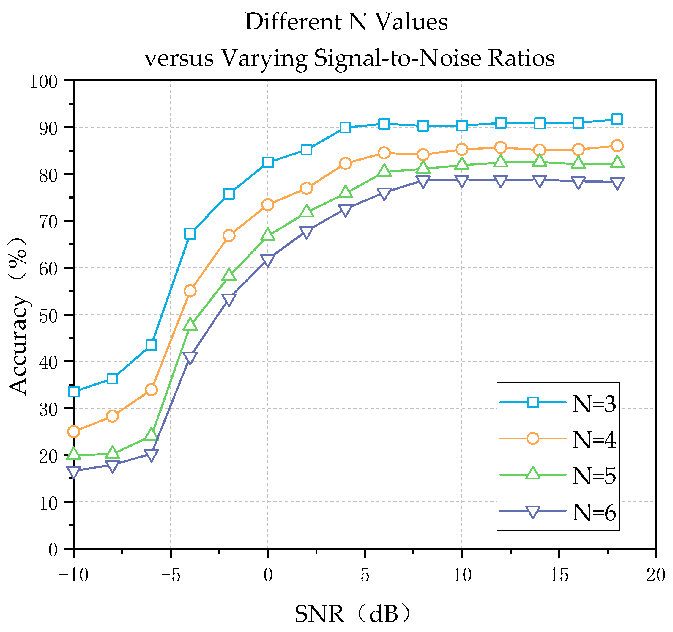
3.4. Performance Comparison for Different Values of N

In this section, we investigate the impact of the number of different class samples in the support set, denoted as N, on the network’s recognition accuracy under the N-way 5-shot setting. For each value of N, namely N = 3, 4, 5, and 6, multiple training sessions were conducted, and the average values were computed. The simulation results are shown in Figure 7.

From Figure 7, it can be observed that as the number of class samples N increases, the performance of the network decreases. When N = 3, the recognition accuracy at 18 dB reaches 91.70%. But when N = 6, the recognition accuracy only reaches 78.36%. With an increase in N, this makes the classification task more complex. This complexity challenges the convergence performance of network training and increases the difficulty of learning for the network model. Additionally, as the differences between classes may become more subtle, the model requires stronger representation learning ability and generalization capability to achieve good performance on new tasks, ultimately leading to a decrease in recognition performance. However, with excessively small values of N, the model only needs to learn a few classes, which may result in overfitting.

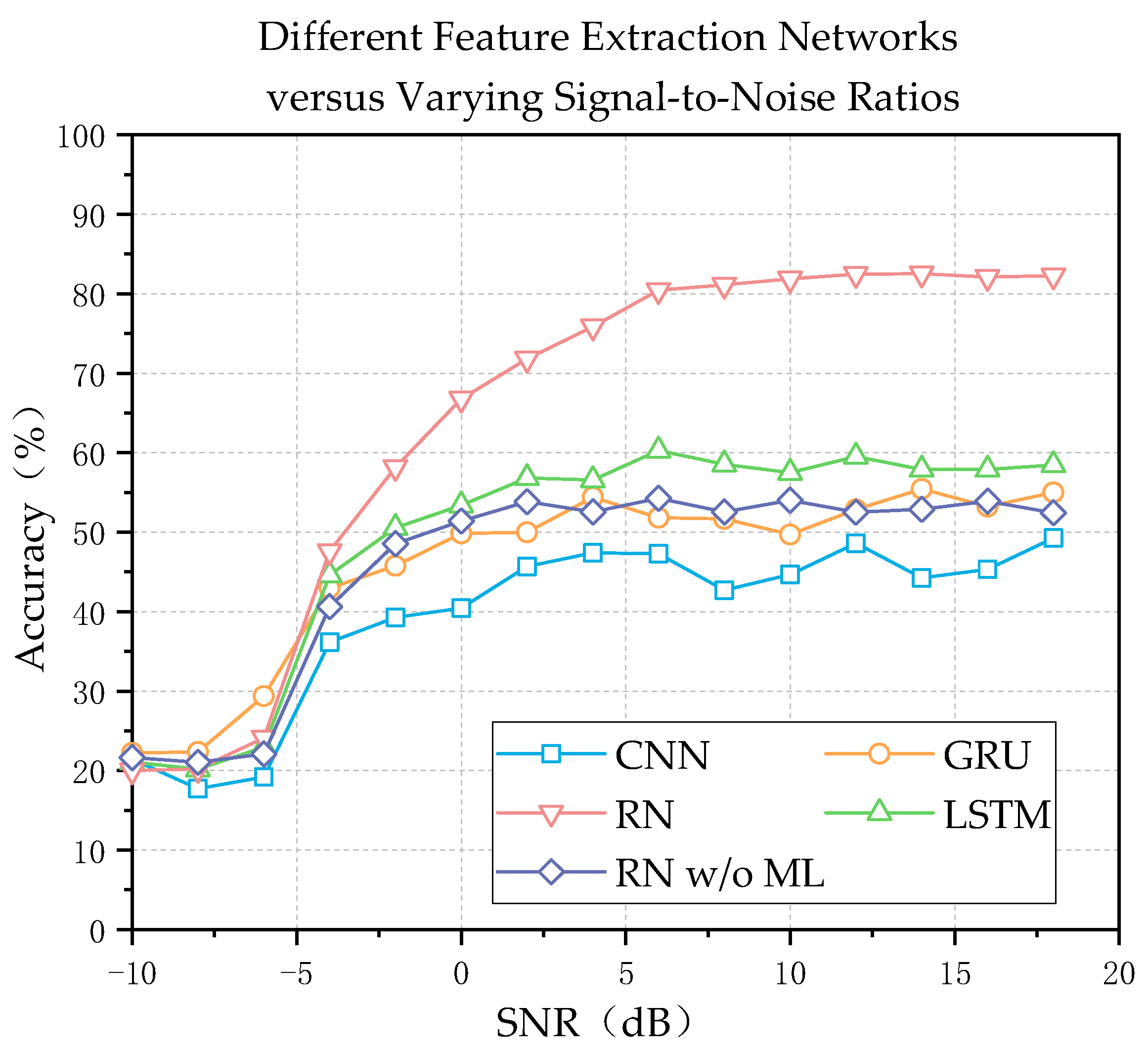
3.5. Performance Analysis with Traditional Methods

In this section, we conduct a performance comparison between the proposed method and traditional networks under the condition of few-shot learning. The compared methods include CNN [31], LSTM [32], and Gated Recurrent Unit (GRU) [33]. The objective is to verify whether the proposed method exhibits strong robustness and generalization capability in handling few-shot problems and whether it outperforms traditional network structures. The traditional networks extracted 600 samples in each training session, while the proposed method is evaluated under the 5-way 5-shot condition with 100 samples. The recognition accuracies of each method as the SNR ratio varies are shown in Figure 8.

It is observed that LSTM and GRU employed gating mechanisms to selectively retain and forget information, enabling them to possess strong contextual memory capabilities. This, in turn, led to better results in the test outcomes compared to traditional CNN. Due to the ability of LSTM’s memory cells to effectively retain and update long-term information, it is suitable for conducting in-depth analysis on long sequences. In contrast, GRU has only one hidden state, resulting in slightly inferior performance compared to LSTM. In contrast to conventional machine learning networks, the approach utilized in this study effectively leveraged the distinctive features of the communication signals and enhanced the model’s learning ability. Our method demonstrated improved accuracy compared to traditional neural networks. Meanwhile, traditional methods still exhibited fluctuations within a broad range, potentially stemming from the limitations in handling small-sample training and model structures inherent in these approaches. This rendered traditional methods more susceptible to disturbances caused by a limited number of samples, resulting in unstable outcomes.

In addition to comparing with traditional methods, such as CNN, LSTM, and GRU, we introduced a comparison with an intermediate approach between the traditional methods and the model proposed in this paper. This approach utilizes the same feature extraction and classification techniques as relation network, but it does not employ an epoch-based training strategy like our proposed model. Instead, it follows the training strategy of traditional machine learning methods, without resorting to meta-learning techniques. From the experimental results, it is evident that even when employing similar feature extraction and classification techniques, not using a meta-learning training strategy still hinders the attainment of the desired level of classification accuracy. This further underscores the advantage of the approach proposed in this paper in addressing the few-shot AMC problem.

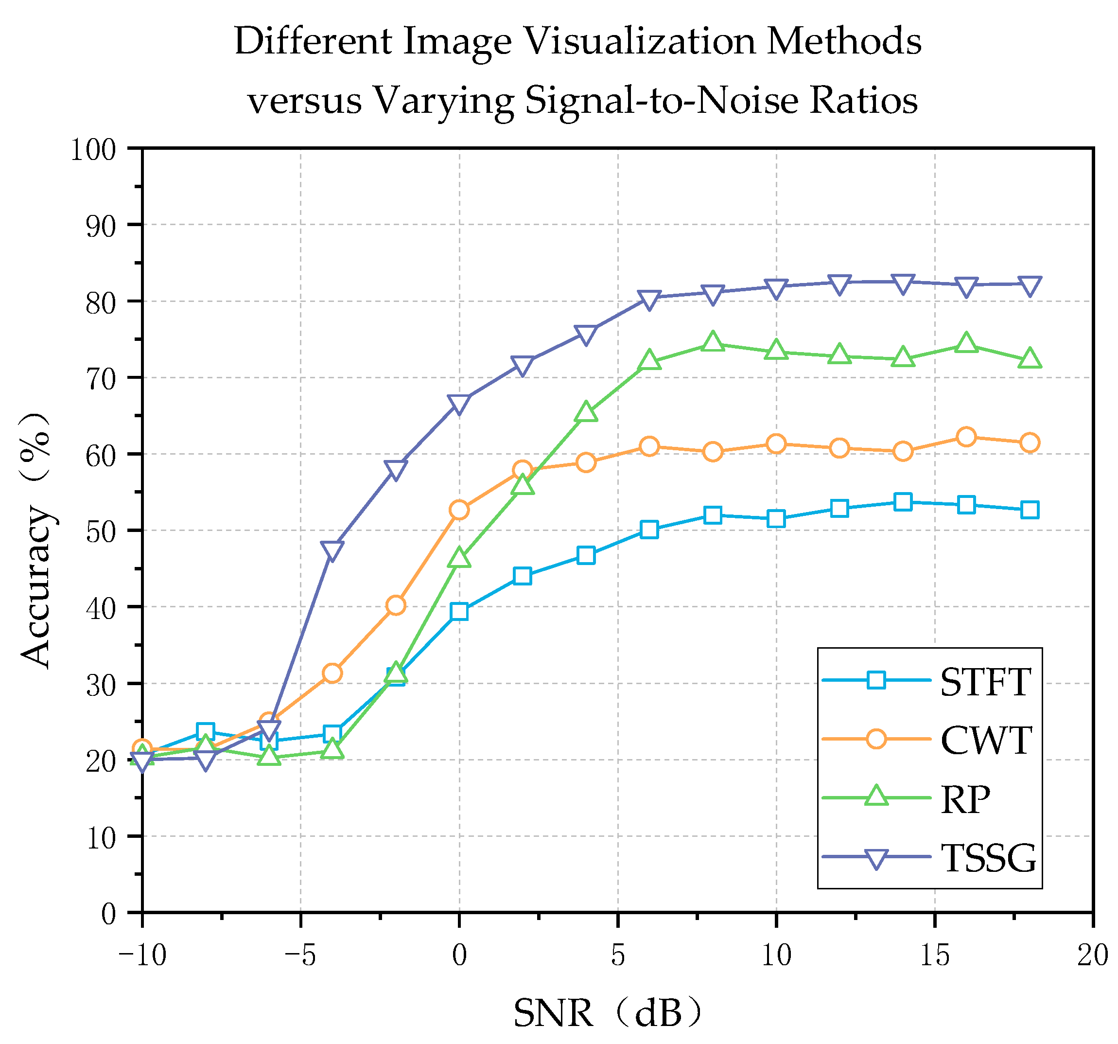
3.6. Comparative Experiment with Other Visualization Methods

In this section, we compare the TSSG representation method, with traditional approaches, such as STFT, Continuous Wavelet Transform (CWT), and RP. We transformed randomly selected signals into recognizable images using each of the four methods. These transformed images were then fed into a relation network with the same set of parameters for feature extraction and classification. The simulation results are illustrated in Figure 9.

The proposed TSSG method exhibits certain advantages over other methods. Compared to the alternatives, TSSG can achieve convergence at lower SNRs, making it more efficient in practical applications. However, in the experiments conducted in this section, STFT and CWT demonstrated relatively poor performance. This may be attributed to the limitations of these methods in handling non-stationary signals, as they struggle to capture the time-varying characteristics of the signals and provide sufficient information for effective feature extraction and classification. On the other hand, the RP method achieved relatively high accuracy under high SNR ratio conditions. However, the recognition accuracy showed slower improvement with increasing SNR ratio.

4. Conclusions

In this paper, we propose a signal transformation method named TSSG and integrate it with meta-learning to address the few-shot AMC problem. The TSSG technique enables the extraction of features between signals with different modulations, while the meta-learning component effectively confronts the challenge of limited labeled samples in a few-shot scenario. Experiments demonstrate that the proposed few-shot AMC approach outperforms classical deep learning methods in terms of classification accuracy. However, performing SSA on signals demands significant computational resources, and accuracy tends to diminish under low SNR. Our future work aims to enhance SSA efficiency and accuracy through dynamic adjustments of functions and improved feature extraction under low SNR.

References

1. Shafi, M.; Molisch, A.F.; Smith, P.J.; Haustein, T.; Zhu, P.; De Silva, P.; Tufvesson, F.; Benjebbour, A.; Wunder, G. 5g: A tutorial overview of standards, trials, challenges, deployment, and practice. IEEE J. Sel. Areas Commun. 2017, 35, 1201–1221. [Google Scholar] [CrossRef]
2. Qin, Z.; Zhou, X.; Zhang, L.; Gao, Y.; Liang, Y.C.; Li, G.Y. 20 Years of Evolution from Cognitive to Intelligent Communications. IEEE Trans. Cogn. Commun. Netw. 2020, 6, 6–20. [Google Scholar] [CrossRef]
3. Mendis, G.J.; Wei, J.; Madanayake, A. Deep learning-based automated modulation classification for cognitive radio. In Proceedings of the 2016 IEEE International Conference on Communication Systems (ICCS), Shenzhen, China, 14–16 December 2016; IEEE: Shenzhen, China, 2016; pp. 1–6. [Google Scholar]
4. Grajal, J.; Yeste-Ojeda, O.; Sanchez, M.A.; Garrido, M.; López-Vallejo, M. Real-time FPGA implementation of an automatic modulation classifier for electronic warfare applications. In Proceedings of the 2011 19th European Signal Processing Conference, Barcelona, Spain, 29 August–2 September 2011; IEEE: Barcelona, Spain, 2011; pp. 1514–1518. [Google Scholar]
5. Liao, K.; Zhao, Y.; Gu, J.; Zhang, Y.; Zhong, Y. Sequential convolutional recurrent neural networks for fast automatic modulation classification. IEEE Access 2021, 9, 27182–27188. [Google Scholar] [CrossRef]
6. European Centre for Disease Prevention and Control (ECDC); European Food Safety Authority (EFSA); European Medicines Agency (EMA). Ecdc/efsa/ema second joint report on the integrated analysis of the consumption of antimicrobial agents and occurrence of antimicrobial resistance in bacteria from humans and food-producing animals: Joint interagency antimicrobial consumption and resistance analysis (jiacra) report. EFSA J. 2017, 15, e04872. [Google Scholar]
7. Zhang, K.; Xu, E.L.; Feng, Z.; Zhang, P. A Dictionary Learning Based Automatic Modulation Classification Method. IEEE Access 2018, 6, 5607–5617. [Google Scholar] [CrossRef]
8. Kim, K.; Polydoros, A. Digital modulation classification: The BPSK versus QPSK case. In Proceedings of the MILCOM 88, 21st Century Military Communications—What’s Possible?’. Conference Record. Military Communications Conference, Piscataway, NJ, USA, 23–26 October 1988; IEEE: Piscataway, NJ, USA, 1988; pp. 431–436. [Google Scholar]
9. Lay, N.E.; Polydoros, A. Modulation classification of signals in unknown ISI environments. In Proceedings of the MILCOM ’95, Piscataway, NJ, USA, 5–8 November 1995; IEEE: Piscataway, NJ, USA, 1995; pp. 170–174. [Google Scholar]
10. Panagiotou, P.; Anastasopoulos, A.; Polydoros, A. Likelihood ratio tests for modulation classification. In MILCOM 2000 Proceedings. 21st Century Military Communications. Architectures and Technologies for Information Superiority (Cat. No.00CH37155); IEEE: Piscataway, NJ, USA, 2000; pp. 670–674. [Google Scholar]
11. Zhang, J.; Wang, B.; Wang, Y.; Liu, M. An Algorithm for OFDM Signal Modulation Recognition and Parameter Estimation under α-Stable Noise. J. Electron. 2018, 46, 1390–1396. [Google Scholar]
12. Yan, X.; Feng, G.; Wu, H.C.; Xiang, W.; Wang, Q. Innovative robust modulation classification using graph-based cyclic-spectrum analysis. IEEE Commun. Lett. 2017, 21, 16–19. [Google Scholar] [CrossRef]
13. Majhi, S.; Gupta, R.; Xiang, W.; Glisic, S. Hierarchical hypothesis and feature-based blind modulation classification for linearly modulated signals. IEEE Trans. Veh. Technol. 2017, 66, 11057–11069. [Google Scholar] [CrossRef]
14. O’Shea, T.J.; Corgan, J.; Clancy, T.C. Convolutional radio modulation recognition networks. In Proceedings of the Engineering Applications of Neural Networks: 17th International Conference, EANN 2016, Aberdeen, UK, 2–5 September 2016; Springer: Berlin/Heidelberg, Germany, 2016; pp. 213–226. [Google Scholar]
15. Huynh-The, T.; Hua, C.-H.; Pham, Q.-V.; Kim, D.-S. MCNet: An efficient CNN architecture for robust automatic modulation classification. IEEE Commun. Lett. 2020, 24, 811–815. [Google Scholar] [CrossRef]
16. Perenda, E.; Rajendran, S.; Pollin, S. Automatic modulation classification using parallel fusion of convolutional neural networks. In Proceedings of the BalkanCom’ 19, Skopje, North Macedonia, 10–12 June 2019. [Google Scholar]
17. Peng, C.; Cheng, W.; Song, Z.; Dong, R. A noise-robust modulation signal classification method based on continuous wavelet transform. In Proceedings of the 2020 IEEE 5th Information Technology and Mechatronics Engineering Conference (ITOEC), Chongqing, China, 12–14 June 2020; pp. 745–750. [Google Scholar]
18. Wang, Z.; Oates, T. Imaging Time-Series to Improve Classification and Imputation. arXiv 2015, arXiv:1506.00327. [Google Scholar]
19. Hatami, N.; Gavet, Y.; Debayle, J. Classification of Time-Series Images Using Deep Convolutional Neural Networks. In Proceedings of the 10th International Conference on Machine Vision (ICMV 2017), Vienna, Austria, 13–15 November 2017. [Google Scholar]
20. Krizhevsky, A.; Sutskever, I.; Hinton, G. ImageNet Classification with Deep Convolutional Neural Networks. In Advances in Neural Information Processing Systems 25 (NIPS 2012); Neural Information Processing Systems Foundation: San Diego, CA, USA, 2012. [Google Scholar]
21. Cha, X.; Peng, H.; Qin, X. Modulation Recognition Method Based on Multi-Branch Convolutional Neural Networks. J. Commun. 2019, 40, 30–37. (In Chinese) [Google Scholar]
22. Liu, M.Q.; Zheng, S.F.; Li, B.B. MPSK Signal Modulation Recognition Based on Deep Learning. J. Natl. Univ. Def. Technol. 2019, 41, 153–158. (In Chinese) [Google Scholar]
23. Vinyals, O.; Blundell, C.; Lillicrap, T.; Wierstra, D. Matching networks for one-shot learning. In Advances in Neural Information Processing Systems 29 (NIPS 2016); Neural Information Processing Systems Foundation: San Diego, CA, USA, 2016. [Google Scholar]
24. Snell, J.; Swersky, K.; Zemel, R. Prototypical networks for few-shot learning. In Advances in Neural Information Processing Systems 30; Neural Information Processing Systems Foundation: San Diego, CA, USA, 2017. [Google Scholar]
25. Sung, F.; Yang, Y.; Zhang, L.; Xiang, T.; Torr, P.H.; Hospedales, T.M. Learning to compare: Relation network for few-shot learning. In Proceedings of the IEEE Conference on Computer Vision and Pattern Recognition, Salt Lake City, UT, USA, 18–23 June 2018; pp. 1199–1208. [Google Scholar]
26. Finn, C.; Abbeel, P.; Levine, S. Model-agnostic meta-learning for fast adaptation of deep networks. In Proceedings of the International Conference on Machine Learning PMLR, Sydney, Australia, 6–11 August 2017; pp. 1126–1135. [Google Scholar]
27. Nichol, A.; Achiam, J.; Schulman, J. On First-Order Meta-Learning Algorithms. arXiv 2018, arXiv:1803.02999. [Google Scholar]
28. Rusu, A.A.; Rao, D.; Sygnowski, J.; Vinyals, O.; Pascanu, R.; Osindero, S.; Hadsell, R. Meta-learning with latent embedding optimization. arXiv 2018, arXiv:1807.05960. [Google Scholar]
29. Hu, J.; Shen, L.; Albanie, S.; Sun, G.; Wu, E. Squeeze-and-Excitation Networks. In Proceedings of the IEEE Conference on Computer Vision and Pattern Recognition (CVPR), Salt Lake City, UT, USA, 18–23 June 2018. [Google Scholar]
30. Kingma, D.P.; Ba, J.L. Adam: A method for stochastic optimization. In Proceedings of the 3rd International Conference on Learning Representations, San Diego, CA, USA, 7–9 May 2015. [Google Scholar]
31. LeCun, Y.; Bengio, Y.; Hinton, G. Deep learning. Nature 2015, 521, 436–444. [Google Scholar] [CrossRef] [PubMed]
32. Hochreiter, S.; Schmidhuber, J. Long short-term memory. Neural Comput. 1997, 9, 1735–1780. [Google Scholar] [CrossRef] [PubMed]
33. Huang, S.; Dai, R.; Huang, J.; Yao, Y.; Gao, Y.; Ning, F.; Feng, Z. Automatic modulation classification using gated recurrent residual network. IEEE Internet Things J. 2020, 7, 7795–7807. [Google Scholar] [CrossRef]
Figure 1. Flowchart of the algorithm.
Applsci 13 09858 g001
Figure 2. Converted four different signals to TSSG. In the waveform plot, the red line represents the I channel of the signal, and the blue line represents the Q channel. In the TSSG, the left side corresponds to the I channel, and the right side corresponds to the Q channel. (a) 32PSK; (b) QPSK; (c) OOK; (d) 64QAM.
Applsci 13 09858 g002aApplsci 13 09858 g002b
Figure 3. RadioML.2018.01a dataset structure. In the waveform plot, the red line represents the I channel of the signal, and the blue line represents the Q channel.
Applsci 13 09858 g003
Figure 4. Loss and accuracy of the model under the two classic conditions of 5-way 5-shot and 5-way 1-shot. (a) Loss and accuracy under the 5-way 1-shot condition; (b) loss and accuracy under the 5-way 5-shot condition.
Applsci 13 09858 g004
Figure 5. Loss and accuracy of the model under four typical signal-to-noise ratios: −4 dB, 0 dB, 6 dB, and 18 dB. (a) Loss and accuracy under the 5-way 1-shot condition; (b) loss and accuracy under the 5-way 5-shot condition.
Applsci 13 09858 g005
Figure 6. Variation of recognition accuracy with SNR ratio for different K values.
Applsci 13 09858 g006
Figure 7. Variation of recognition accuracy with SNR ratio for different N values.
Applsci 13 09858 g007
Figure 8. Comparison of recognition accuracy with traditional methods under small sample conditions.
Applsci 13 09858 g008
Figure 9. Comparison of recognition accuracy with conventional pictorial methods under small sample conditions.
Applsci 13 09858 g009