
Hyperspectral Imaging for Fresh-Cut Fruit and Vegetable Quality Assessment: Basic Concepts and Applications

 ,
,  ,
,  , ,
, ,  ,
,  and
and 
Abstract
:1. Introduction
2. HSI: Basic Concepts
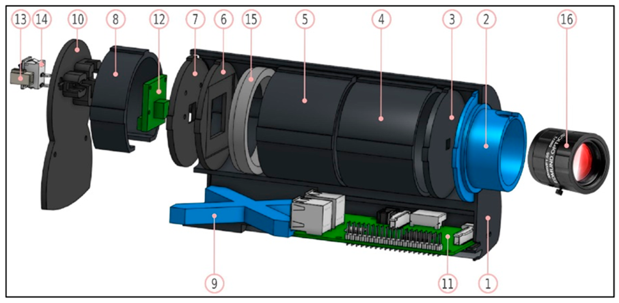
2.1. HSI: Device Components
2.1.1. Light Source
2.1.2. Wavelength Dispersion Systems
2.1.3. Detectors
2.2. Image Sensing and Acquisition Modes
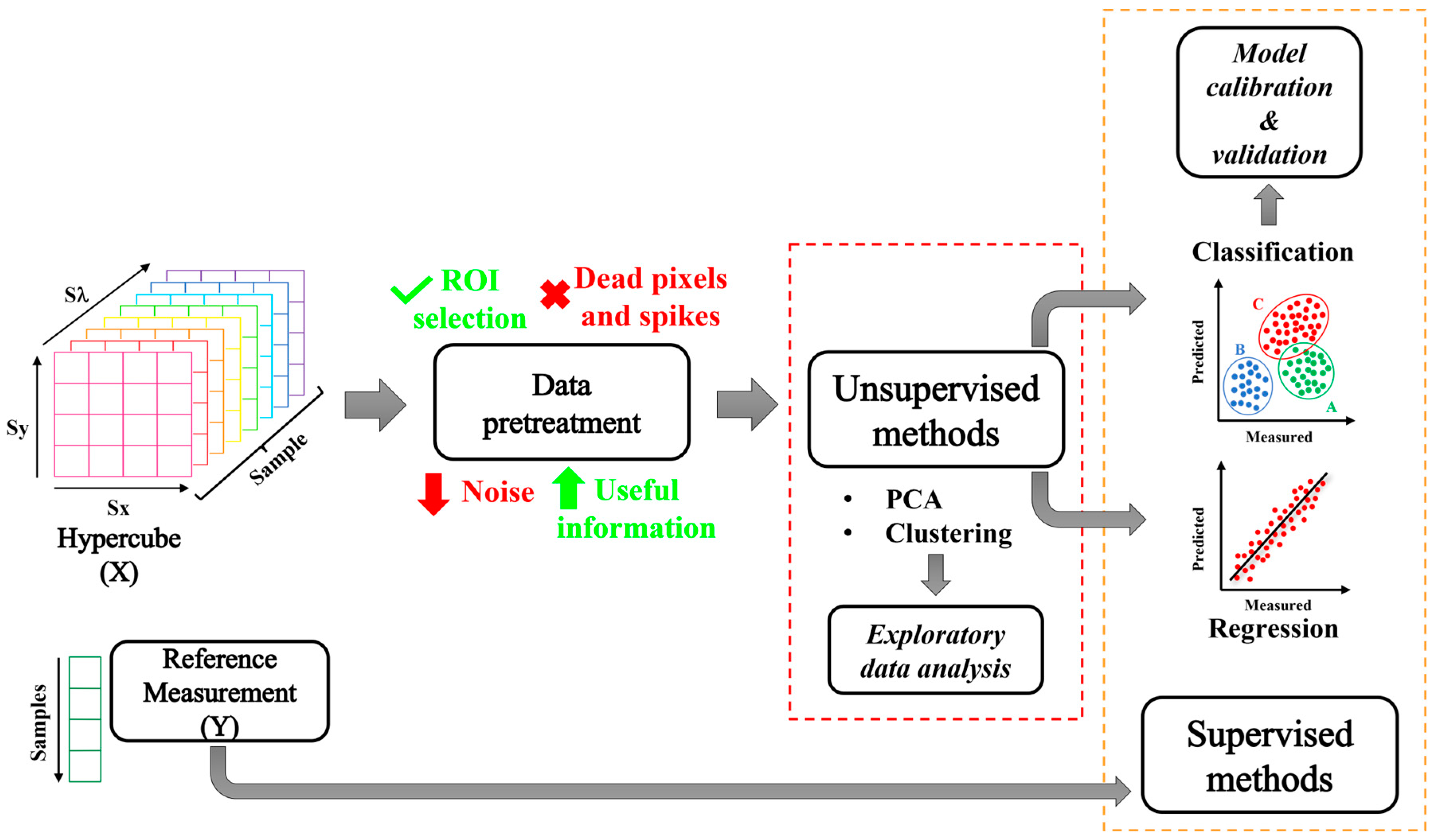
3. Software and Image Processing
3.1. Multivariate Statistical Analyses
3.1.1. Unsupervised Methods
3.1.2. Supervised Methods

| Method 1 | Reference | |
|---|---|---|
| Classification | PLS-DA | Diezma et al. [29], Everard et al. [30], Rady et al. [31], Pu et al. [32], Zhu et al. [33], Babellahi et al. [34] |
| LDA | Lee et al. [35], Delwiche et al. [36] | |
| KNN | Rady et al. [31], Pu et al. [32], | |
| SIMCA | Pu et al. [32], Ríos-Reina et al. [37] | |
| SVM | Cen et al. [38], Zhu et al. [33], Bai et al. [39] | |
| Regression | PCR | van Roy et al. [40], Xu et al. [41] |
| PLSR | Rady et al. [31], van Roy et al. [40], Yan et al. [42], Amodio et al. [43], Mo et al. [44], Zhu et al. [45], Rahman et al. [46], Ramos-Infante et al. [47], Chaudhry et al. [48], Xiao et al. [49], Babellahi et al. [34], Shrestha et al. [50], Eshkabilov et al. [51], Wang et al. [52], Li et al. [53], Lan et al. [54], Xu et al. [41] | |
| MLR | Lu and Peng [55], Peng and Lu [56], Rajkumar et al. [57], Zhu et al. [45] | |
| ANNs | Siripatrawan et al. [58], Li et al. [53] | |
| SVR | Zhang et al. [59], Chen et al. [60], Pang et al. [61] | |
| LS-SVM | Zhu et al. [45], Xiao et al. [49] | |
4. HSI in Fresh-Cut Product Quality Assessment
4.1. Fresh-Cut Green Leafy Vegetables
4.1.1. Lettuce
4.1.2. Spinach Leaves
4.1.3. Rocket
4.2. Fresh-Cut Tubers
Potatoes
4.3. Fresh-Cut Fruits
4.3.1. Tomato
4.3.2. Cucumber
4.3.3. Green Bell Pepper
4.3.4. Apple
4.4. Fresh-Cut Vegetables
4.4.1. Celery
4.4.2. Cabbage, Carrot, Green Onion, Onion, Potato, Radish, and Zucchini
| Fresh-Cut Product | Quality Features | Spectral Range | Sensing Mode | Modeling Method | Performances | Reference |
|---|---|---|---|---|---|---|
| Lettuce | Color | 400–1000 nm | Reflectance | Classification SI and RI | Accuracy, sensitivity, and specificity > 99.9% | Mo et al. [69] |
| Color–Browning | 400–1000 nm | Reflectance | ANOVA, Classification SI and RI | Accuracy = 97.0–100.0% | Mo et al. [79] | |
| Decay | 380–1012 nm | Reflectance and Chlorophyll Fluorescence | Classification | Accuracy = 97.0% | Simko et al. [71] | |
| Relative water content, chlorophyll, and carotenoid | 400–1000 nm | Reflectance | Wavelength ratio | – | Shurygin et al. [80] | |
| Nutrient levels: NO3−, Ca2+, K+, SSC, pH, SPAD | 400–1000 nm | Reflectance | PLSR, PCA | R2 = 0.78–0.99 | Eshkabilov et al. [51] | |
| Fecal contamination | 400–800 nm | Fluorescence | Classification RI | Accuracy = 80.0–100.0% | Cho et al. [72] | |
| Foreign substances (slugs and worms) | 400–1000 nm | Reflectance | Classification SI and RI | Accuracy = 97.5%, sensitivity = 98.0%, and specificity = 97.0% with SI Accuracy = 99.5%, sensitivity = 100.0%, and specificity = 99.0% with RI | Mo et al. [70] | |
| Foreign substances (worms) | 400–1000 nm, 980–1700 nm | Reflectance | Classification SI and RI | Accuracy of 97.0% for Vis/NIR imaging and 100.0% for NIR imaging | Mo et al. [81] | |
| Spinach leaves | Shelf life | 400–1000 nm | Reflectance | Classification SAM, PLS-DA, and LEVE index | Over 95.0% of the leaves were classified into the same quality class by SAM and LEVE index | Diezma et al. [29] |
| Shelf life and freshness (under plastic film) | 400–1000 nm | Reflectance | PCA + ANOVA | Freshness characterization over time | Lara et al. [82] | |
| Shelf life and freshness | 380–1030 nm, 874–1734 nm | Reflectance | PLS-DA, SVM, ELM | Accuracy > 92.0% | Zhu et al. [33] | |
| Escherichia coli | 400–1000 nm | Reflectance | ANN | R2 = 0.97 | Siripatrawan et al. [58] | |
| Fecal contamination | 456–950 nm 464–800 nm | Reflectance Fluorescence | PLS-DA | Fluorescence had the best results with accuracy from 87.0% to 100.0% | Everard et al. [30] | |
| Rocket | Shelf life | 400–1000 nm | Reflectance | PLSR | R2 = 0.73–0.95 | Chaudhry et al. [73] |
| Vitamin C and phenols | 400–1000 nm 900–1700 nm | Reflectance | PLSR |
| Chaudhry et al. [48] | |
| Green amaranth leaves | Chlorophyll content | 400–1000 nm | Reflectance | PLSR | R2 = 0.834 RMSE = 0.067% | Mardhiyatna et al. [83] |
| Potato slices | Color and water content | 400–1000 nm | Reflectance | PLS, SVM, and LS-SVM | LS-SVM had the best performances with R2 above 0.80 for the prediction of both parameters | Xiao et al. [49] |
| Starch content | 380–1000 nm | Reflectance | PLSR | R2 = 0.95 RMSEP = 1.63 g kg−1 RPD = 2.95 | Wang et al. [52] | |
| Escherichia coli | 400–1000 nm | Reflectance | PLSR, BP-NN | BP-NN model reached the best performances using both the full spectrum (R2 = 0.97; RMSEP = 0.065 log CFU g−1) and selected wavelengths (R2 = 0.88; RMSEP =0.142 log CFU g−1) | Li et al. [53] | |
| Sulfur dioxide residue | 975–1646 nm | Reflectance | SVM | Classification accuracy of 95.0% | Bai et al. [39] | |
| Tomato | Color | 325–985 nm | Reflectance | PLSR, PCR | For a*, hue, and L*, R2 > 0.86; for b* and chroma, R2 = 0.4–0.5 | van Roy et al. [40] |
| Cracking defects | 1000–1700 nm | Reflectance | LDA | Accuracy of 91.7% (using full NIR spectrum) and of 80.6% (using only 4 wavelengths) | Lee et al. [35] | |
| Cracking defects | 400–700 nm | Fluorescence | ANOVA + PCA | Accuracy >99.0% | Cho et al. [84] | |
| Firmness and sweetness | 1000–1550 nm | Reflectance | PLSR |
| Rahman et al. [46] | |
| Firmness, color, pH, and SSC | 400–1000 nm, 900–1700 nm | Reflectance | PLSR | Good performances in prediction were achieved:
| Ramos-Infante et al. [47] | |
| Cucumber | Chilling injury | 500–675 nm 675–1000 nm | Reflectance Transmittance | NB, SVM, KNN | SVM was the best, achieving an accuracy from 90.5% to 100% | Cen et al. [38] |
| Green bell pepper | Shelf life | 464–799 nm | Fluorescence | LDA | LDA was successful in distinguishing the storage time at 0, 7, 14, and 21 days after cutting | Delwiche et al. [36] |
| Chilling injury | 400–1000 nm, 1000–2500 nm | Reflectance | PLS-DA | NERCV = 83% with Vis-NIR model. NERCV = 81% with NIR model | Babellahi et al. [34] | |
| PLSR | R2CV = 0.79, RMSECV = 0.5 days of storage at 4 °C | |||||
| Apple | SSC | 400–1000 nm | Reflectance | PLSR | The best-performing models were
| Mo et al. [44] |
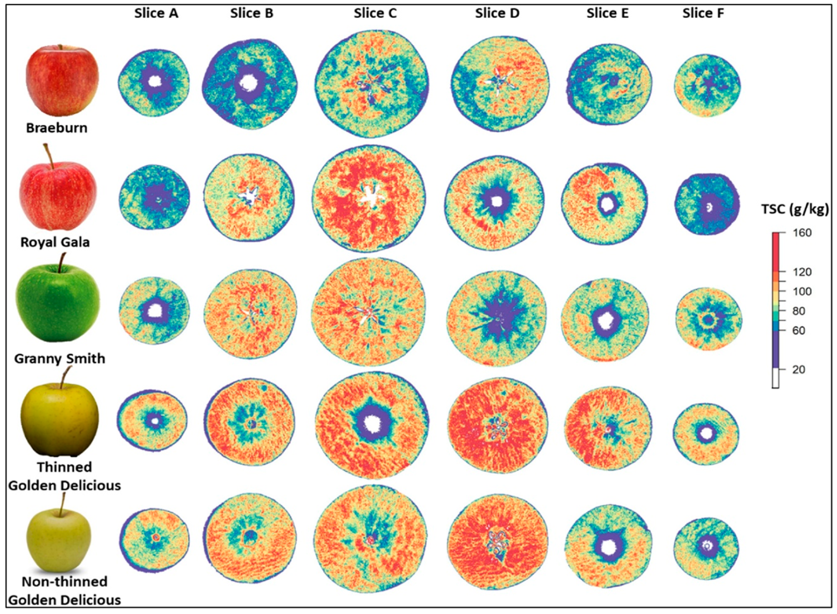
| DMC, TSC | 1000–2500 nm | Reflectance | LOO-PLS |
| Lan et al. [54] | |
| Browning–PPO activity | 400–1000 nm | Reflectance | PLSR | An indirect detection of PPO activity was performed, and the results showed that the changes in the enzyme activity were mainly at wavelengths around 677 nm | Shrestha et al. [50] | |
| Celery | Dietary fiber | 378–1008 nm | Reflectance | PLS, Si-PLS, GA-Si-PLS | GA-Si-PLS had the best performances:
| Yan et al. [42] |
| Fennel | SSC, phenol and antioxidant activity, sugars, and organic acids | 400–1000 nm, 900–1700 nm | Reflectance | PLSR |
| Amodio et al. [43] |
| PLS-DA | NERP = 88.57% | |||||
| Bamboo shoots | Dietary fiber | 400–1000 nm, 900–1700 nm | Reflectance | PLSR, PCR | SNV-PCA-PLSR achieved good prediction performances with R2p = 0.902 and RMSEP = 0.135 | Xu et al. [41] |
| Onion, zucchini, garlic, and carrot | Foreign objects | 420–730 nm | Fluorescence, Reflectance | Wavelength ratio classification method | Accuracy of 90.0–97.0% to detect different kinds of foreign materials | Cho [85] |
| Cabbage, carrot, green onion, onion, potato, radish, and zucchini | Foreign materials | 400–1000 nm, 1000–2500 nm | Reflectance | PLS-DA | Accuracy of 99.0% with SWIR, 89.0% with Vis/NIR, and 64.0% with fluorescence | Tunny et al. [78] |
| 400–1000 nm | Fluorescence |
5. Conclusions and Perspectives
Author Contributions
Funding
Institutional Review Board Statement
Informed Consent Statement
Data Availability Statement
Conflicts of Interest
Abbreviations
| ANN | Artificial Neural Network | NIR | Near-infrared |
| ANOVA | Analysis of Variance | PAT | Process Analytical Technology |
| AOTF | Acousto-Optic Tunable Filter | PC | Principal Component |
| CCD | Charge-Coupled Device | PCA | Principal Component Analysis |
| CFU | Colony-Forming Unit | PCR | Principal Component Regression |
| CMOS | Complementary Metal-Oxide-Semiconductor | PLS-DA | Partial Least Square–Discriminant Analysis |
| CTIS | Computed Tomography Imaging Spectrometer | PLSR | Partial Least Square Regression |
| DMC | Dry Matter Content | PPO | Polyphenol-Oxidase |
| ELM | Extreme Learning Machine | R2 | Coefficient of Determination |
| ETFs | Electronically Tunable Filters | R2CV | Coefficient of Determination in Cross-Validation |
| FMs | Foreign materials | R2p | Coefficient of Determination in Prediction |
| GA-Si-PLS | Genetic Synergy Interval Partial Least Square | RI | Ratio Imaging |
| Ge | Germanium | RMSE | Root Mean Square Error |
| HSI | Hyperspectral Imaging or Hyperspectral Image | RMSECV | Root Mean Square Error in Cross-Validation |
| IDF | Insoluble Dietary Fiber | RMSEP | Root Mean Square Error in prediction |
| InGaAs | Indium Gallium Arsenide | ROI | Region of Interest |
| InSb | Indium Antimonite | SAM | Spectral Angle Mapper |
| IoT | Internet of Things | SDF | Soluble Dietary Fibre |
| KNN | K-Nearest Neighbor | SG | Savitzky–Golay |
| LCTF | Liquid Crystal Tunable Filter | SI | Subtraction Imaging |
| LDA | Linear Discriminant Analysis | Si | Silicon |
| LEDI | Lettuce Decay Index | SIMCA | Soft Independent Modeling by Class Analogy |
| LEDs | Light-Emitting Diodes | Si-PLS | Synergy Interval–Partial Least Square |
| LEVE | Leafy Vegetable Evolution | SNV | Standard Normal Variate |
| LOO-PLS | Leave-One-Out Partial Least Square | SPAD | Soil Plant Analysis Development |
| LS-SVM | Least Square Support Vector Machine | SSC | Soluble Solid Content |
| MAP | Modified Atmosphere Packaging | SVM | Support Vector Machine |
| MLR | Multiple Linear Regression | SVR | Support Vector Machine Regression |
| MSC | Multiplicative Scatter Correction | SWIR | Shortwave Infrared |
| MSPC | Multivariate Statistical Process Control | TSC | Total Sugar Content |
| MTC or HgCdTe | Mercury Cadmium Tellurium | UV | Ultraviolet |
| MVE | Minimum Volume Ellipsoid | VIP | Variable Importance in Projection |
| NB | Naïve Bayes | Vis | Visible |
| NER | Non Error Rate |
References
- Colelli, G.; Elia, A. Physiological and technological aspects of fresh-cut horticultural products. Italus Hortus 2009, 16, 55–78. [Google Scholar]
- Lu, Y.; Saeys, W.; Kim, M.; Peng, Y.; Lu, R. Hyperspectral imaging technology for quality and safety evaluation of horticultural products: A review and celebration of the past 20-year progress. Postharvest Biol. Technol. 2020, 170, 111318. [Google Scholar] [CrossRef]
- Lu, Y.; Huang, Y.; Lu, R. Innovative hyperspectral imaging-based techniques for quality evaluation of fruits and vegetables: A review. Appl. Sci. 2017, 7, 189. [Google Scholar] [CrossRef]
- Wu, D.; Sun, D.W. Advanced applications of hyperspectral imaging technology for food quality and safety analysis and assessment: A review—Part I: Fundamentals. Innov. Food Sci. Emerg. Technol. 2013, 19, 1–14. [Google Scholar] [CrossRef]
- Siche, R.; Vejarano, R.; Aredo, V.; Velasquez, L.; Saldana, E.; Quevedo, R. Evaluation of food quality and safety with hyperspectral imaging (HSI). Food Eng. Rev. 2016, 8, 306–322. [Google Scholar] [CrossRef]
- Lu, B.; Dao, P.D.; Liu, J.; He, Y.; Shang, J. Recent advances of hyperspectral imaging technology and applications in agriculture. Remote Sens. 2020, 12, 2659. [Google Scholar] [CrossRef]
- Gowen, A.A.; O’Donnell, C.P.; Cullen, P.J.; Downey, G.; Frias, J.M. Hyperspectral imaging–an emerging process analytical tool for food quality and safety control. Trends Food Sci. Technol. 2007, 18, 590–598. [Google Scholar] [CrossRef]
- Martinsen, P.; Schaare, P. Measuring soluble solids distribution in kiwifruit using near-infrared imaging spectroscopy. Postharvest Biol. Technol. 1998, 14, 271–281. [Google Scholar] [CrossRef]
- Nicolai, B.M.; Beullens, K.; Bobelyn, E.; Peirs, A.; Saeys, W.; Theron, K.I.; Lammertyn, J. Nondestructive measurement of fruit and vegetable quality by means of NIR spectroscopy: A review. Postharvest Biol. Technol. 2007, 46, 99–118. [Google Scholar] [CrossRef]
- Amigo, J.M.; Grassi, S. Configuration of hyperspectral and multispectral imaging systems. In Data Handling in Science and Technology; Elsevier: Amsterdam, The Netherlands, 2019; Volume 32, pp. 17–34. [Google Scholar]
- Lodhi, V.; Chakravarty, D.; Mitra, P. Hyperspectral imaging system: Development aspects and recent trends. Sens. Imaging 2019, 20, 35. [Google Scholar] [CrossRef]
- Qin, J. Hyperspectral imaging instruments. In Hyperspectral Imaging for Food Quality Analysis and Control; Academic Press: Cambridge, MA, USA, 2010; pp. 129–172. [Google Scholar]
- Marini, F.; Amigo, J.M. Unsupervised exploration of hyperspectral and multispectral images. In Data Handling in Science and Technology; Elsevier: Amsterdam, The Netherlands, 2019; Volume 32, pp. 93–114. [Google Scholar]
- Mobaraki, N.; Amigo, J.M. HYPER-Tools. A graphical user-friendly interface for hyperspectral image analysis. Chemom. Intell. Lab. Syst. 2018, 172, 174–187. [Google Scholar] [CrossRef]
- Laura, J.R.; Gaddis, L.R.; Anderson, R.B.; Aneece, I.P. Introduction to the Python Hyperspectral Analysis Tool (PyHAT). In Machine Learning for Planetary Science; Elsevier: Amsterdam, The Netherlands, 2022; pp. 55–90. [Google Scholar]
- Jiang, H.; Yoon, S.C.; Zhuang, H.; Wang, W.; Li, Y.; Lu, C.; Li, N. Non-destructive assessment of final color and pH attributes of broiler breast fillets using visible and near-infrared hyperspectral imaging: A preliminary study. Infrared Phys. Technol. 2018, 92, 309–317. [Google Scholar] [CrossRef]
- Amigo, J.M.; Santos, C. Preprocessing of hyperspectral and multispectral images. In Data Handling in Science and Technology; Elsevier: Amsterdam, The Netherlands, 2019; Volume 32, pp. 37–53. [Google Scholar]
- Biancolillo, A.; Marini, F. Chemometrics applied to plant spectral analysis. In Comprehensive Analytical Chemistry; Elsevier: Amsterdam, The Netherlands, 2018; Volume 80, pp. 69–104. [Google Scholar]
- Boulet, J.C.; Roger, J.M. Pretreatments by means of orthogonal projections. Chemom. Intell. Lab. Syst. 2012, 117, 61–69. [Google Scholar] [CrossRef]
- Oliveri, P.; Malegori, C.; Simonetti, R.; Casale, M. The impact of signal pre-processing on the final interpretation of analytical outcomes–A tutorial. Anal. Chim. Acta 2019, 1058, 9–17. [Google Scholar] [CrossRef]
- Rinnan, Å. Pre-processing in vibrational spectroscopy–when, why and how. Anal. Methods 2014, 6, 7124–7129. [Google Scholar] [CrossRef]
- Biancolillo, A.; Marini, F.; Ruckebusch, C.; Vitale, R. Chemometric strategies for spectroscopy-based food authentication. Appl. Sci. 2020, 10, 6544. [Google Scholar] [CrossRef]
- Maimon, O.; Rokach, L. Introduction to supervised methods. In Data Mining and Knowledge Discovery Handbook; Springer: Boston, MA, USA, 2005; pp. 149–164. [Google Scholar]
- Nasteski, V. An overview of the supervised machine learning methods. Horizons. b 2017, 4, 51–62. [Google Scholar] [CrossRef]
- de la Ossa, M.Á.F.; Amigo, J.M.; García-Ruiz, C. Detection of residues from explosive manipulation by near infrared hyperspectral imaging: A promising forensic tool. Forensic Sci. Int. 2014, 242, 228–235. [Google Scholar] [CrossRef] [PubMed]
- Torres, I.; Amigo, J.M. An overview of regression methods in hyperspectral and multispectral imaging. Data Handl. Sci. Technol. 2019, 32, 205–230. [Google Scholar]
- Amigo, J.M.; Martí, I.; Gowen, A. Hyperspectral imaging and chemometrics: A perfect combination for the analysis of food structure, composition and quality. In Data Handling in Science and Technology; Elsevier: Amsterdam, The Netherlands, 2013; Volume 28, pp. 343–370. [Google Scholar]
- Liakos, K.G.; Busato, P.; Moshou, D.; Pearson, S.; Bochtis, D. Machine learning in agriculture: A review. Sensors 2018, 18, 2674. [Google Scholar] [CrossRef]
- Diezma, B.; Lleó, L.; Roger, J.M.; Herrero-Langreo, A.; Lunadei, L.; Ruiz-Altisent, M. Examination of the quality of spinach leaves using hyperspectral imaging. Postharvest Biol. Technol. 2013, 85, 8–17. [Google Scholar] [CrossRef]
- Everard, C.D.; Kim, M.S.; Lee, H. A comparison of hyperspectral reflectance and fluorescence imaging techniques for detection of contaminants on spinach leaves. J. Food Eng. 2014, 143, 139–145. [Google Scholar] [CrossRef]
- Rady, A.; Guyer, D.; Lu, R. Evaluation of sugar content of potatoes using hyperspectral imaging. Food Bioprocess Technol. 2015, 8, 995–1010. [Google Scholar] [CrossRef]
- Pu, Y.Y.; Sun, D.W.; Buccheri, M.; Grassi, M.; Cattaneo, T.M.; Gowen, A. Ripeness classification of bananito fruit (Musa acuminata, AA): A comparison study of visible spectroscopy and hyperspectral imaging. Food Anal. Methods 2019, 12, 1693–1704. [Google Scholar] [CrossRef]
- Zhu, S.; Feng, L.; Zhang, C.; Bao, Y.; He, Y. Identifying freshness of spinach leaves stored at different temperatures using hyperspectral imaging. Foods 2019, 8, 356. [Google Scholar] [CrossRef]
- Babellahi, F.; Paliwal, J.; Erkinbaev, C.; Amodio, M.L.; Chaudhry, M.M.A.; Colelli, G. Early detection of chilling injury in green bell peppers by hyperspectral imaging and chemometrics. Postharvest Biol. Technol. 2020, 162, 111100. [Google Scholar] [CrossRef]
- Lee, H.; Kim, M.S.; Jeong, D.; Chao, K.; Cho, B.K.; Delwiche, S.R. Hyperspectral near-infrared reflectance imaging for detection of defect tomatoes. In Sensing for Agriculture and Food Quality and Safety Iii; SPIE: Bellingham, WA, USA, 2011; Volume 8027, pp. 148–156. [Google Scholar]
- Delwiche, S.R.; Stommel, J.R.; Kim, M.S.; Vinyard, B.T.; Esquerre, C. Hyperspectral fluorescence imaging for shelf life evaluation of fresh-cut Bell and Jalapeno Pepper. Sci. Hortic. 2019, 246, 749–758. [Google Scholar] [CrossRef]
- Ríos-Reina, R.; Callejón, R.M.; Amigo, J.M. Feasibility of a rapid and non-destructive methodology for the study and discrimination of pine nuts using near-infrared hyperspectral analysis and chemometrics. Food Control. 2021, 130, 108365. [Google Scholar] [CrossRef]
- Cen, H.; Lu, R.; Zhu, Q.; Mendoza, F. Nondestructive detection of chilling injury in cucumber fruit using hyperspectral imaging with feature selection and supervised classification. Postharvest Biol. Technol. 2016, 111, 352–361. [Google Scholar] [CrossRef]
- Bai, X.; Xiao, Q.; Zhou, L.; Tang, Y.; He, Y. Detection of sulfite dioxide residue on the surface of fresh-cut potato slices using near-infrared hyperspectral imaging system and portable near-infrared spectrometer. Molecules 2020, 25, 1651. [Google Scholar] [CrossRef]
- van Roy, J.; Keresztes, J.C.; Wouters, N.; De Ketelaere, B.; Saeys, W. Measuring colour of vine tomatoes using hyperspectral imaging. Postharvest Biol. Technol. 2017, 129, 79–89. [Google Scholar] [CrossRef]
- Xu, X.Y.; Xie, W.G.; Xiang, C.; You, Q.; Tian, X.G. Predicting the dietary fiber content of fresh-cut bamboo shoots using a visible and near-infrared hyperspectral technique. J. Food Meas. Charact. 2023, 17, 3218–3227. [Google Scholar] [CrossRef]
- Yan, L.; Xiong, C.; Qu, H.; Liu, C.; Chen, W.; Zheng, L. Non-destructive determination and visualisation of insoluble and soluble dietary fibre contents in fresh-cut celeries during storage periods using hyperspectral imaging technique. Food Chem. 2017, 228, 249–256. [Google Scholar] [CrossRef]
- Amodio, M.L.; Capotorto, I.; Chaudhry, M.M.A.; Colelli, G. The use of hyperspectral imaging to predict the distribution of internal constituents and to classify edible fennel heads based on the harvest time. Comput. Electron. Agric. 2017, 134, 1–10. [Google Scholar] [CrossRef]
- Mo, C.; Kim, M.S.; Kim, G.; Lim, J.; Delwiche, S.R.; Chao, K.; Lee, H.; Cho, B.K. Spatial assessment of soluble solid contents on apple slices using hyperspectral imaging. Biosyst. Eng. 2017, 159, 10–21. [Google Scholar] [CrossRef]
- Zhu, H.; Chu, B.; Fan, Y.; Tao, X.; Yin, W.; He, Y. Hyperspectral imaging for predicting the internal quality of kiwifruits based on variable selection algorithms and chemometric models. Sci. Rep. 2017, 7, 1–13. [Google Scholar] [CrossRef]
- Rahman, A.; Park, E.; Bae, H.; Cho, B.K. Hyperspectral imaging technique to evaluate the firmness and the sweetness index of tomatoes. Korean J. Agric. Sci. 2018, 45, 823–837. [Google Scholar]
- Ramos-Infante, S.J.; Suárez-Rubio, V.; Luri-Esplandiu, P.; Sáiz-Abajo, M.J. Assessment Of Tomato Quality Characteristics Using Vis/Nir Hyperspectral Imaging and Chemometrics. In Proceedings of the 2019 10th Workshop on Hyperspectral Imaging and Signal Processing: Evolution in Remote Sensing (WHISPERS), Amsterdam, The Netherlands, 24–26 September 2019; IEEE: Piscataway, NJ, USA; pp. 1–5. [Google Scholar]
- Chaudhry, M.M.; Amodio, M.L.; Amigo, J.M.; de Chiara, M.L.; Babellahi, F.; Colelli, G. Feasibility study for the surface prediction and mapping of phytonutrients in minimally processed rocket leaves (Diplotaxis tenuifolia) during storage by hyperspectral imaging. Comput. Electron. Agric. 2020, 175, 105575. [Google Scholar] [CrossRef]
- Xiao, Q.; Bai, X.; He, Y. Rapid screen of the color and water content of fresh-cut potato tuber slices using hyperspectral imaging coupled with multivariate analysis. Foods 2020, 9, 94. [Google Scholar] [CrossRef]
- Shrestha, L.; Kulig, B.; Moscetti, R.; Massantini, R.; Pawelzik, E.; Hensel, O.; Sturm, B. Comparison between hyperspectral imaging and chemical analysis of polyphenol oxidase activity on fresh-cut apple slices. J. Spectrosc. 2020, 2020, 7012525. [Google Scholar] [CrossRef]
- Eshkabilov, S.; Lee, A.; Sun, X.; Lee, C.W.; Simsek, H. Hyperspectral imaging techniques for rapid detection of nutrient content of hydroponically grown lettuce cultivars. Comput. Electron. Agric. 2021, 181, 105968. [Google Scholar] [CrossRef]
- Wang, F.; Wang, C.; Song, S. A study of starch content detection and the visualization of fresh-cut potato based on hyperspectral imaging. RSC Adv. 2021, 11, 13636–13643. [Google Scholar] [CrossRef] [PubMed]
- Li, D.; Zhang, F.; Yu, J.; Chen, X.; Liu, B.; Meng, X. A rapid and non-destructive detection of Escherichia coli on the surface of fresh-cut potato slices and application using hyperspectral imaging. Postharvest Biol. Technol. 2021, 171, 111352. [Google Scholar] [CrossRef]
- Lan, W.; Jaillais, B.; Renard, C.M.; Leca, A.; Chen, S.; Le Bourvellec, C.; Bureau, S. A method using near infrared hyperspectral imaging to highlight the internal quality of apple fruit slices. Postharvest Biol. Technol. 2021, 175, 111497. [Google Scholar] [CrossRef]
- Lu, R.; Peng, Y. Hyperspectral scattering for assessing peach fruit firmness. Biosyst. Eng. 2006, 93, 161–171. [Google Scholar] [CrossRef]
- Peng, Y.; Lu, R. Analysis of spatially resolved hyperspectral scattering images for assessing apple fruit firmness and soluble solids content. Postharvest Biol. Technol. 2008, 48, 52–62. [Google Scholar] [CrossRef]
- Rajkumar, P.; Wang, N.; EImasry, G.; Raghavan, G.S.V.; Gariepy, Y. Studies on banana fruit quality and maturity stages using hyperspectral imaging. J. Food Eng. 2012, 108, 194–200. [Google Scholar] [CrossRef]
- Siripatrawan, U.; Makino, Y.; Kawagoe, Y.; Oshita, S. Rapid detection of Escherichia coli contamination in packaged fresh spinach using hyperspectral imaging. Talanta 2011, 85, 276–281. [Google Scholar] [CrossRef] [PubMed]
- Zhang, H.; Paliwal, J.; Jayas, D.S.; White, N.D.G. Classification of fungal infected wheat kernels using near-infrared reflectance hyperspectral imaging and support vector machine. Trans. ASABE 2007, 50, 1779–1785. [Google Scholar] [CrossRef]
- Chen, S.; Zhang, F.; Ning, J.; Liu, X.; Zhang, Z.; Yang, S. Predicting the anthocyanin content of wine grapes by NIR hyperspectral imaging. Food Chem. 2015, 172, 788–793. [Google Scholar] [CrossRef]
- Pang, T.; Rao, L.; Chen, X.; Cheng, J. Impruved prediction of soluble solid content of apple using a combination of spectral and textural features of hyperspectral images. J. Appl. Spectrosc. 2021, 87, 1196–1205. [Google Scholar] [CrossRef]
- Francis, G.A.; Gallone, A.; Nychas, G.J.; Sofos, J.N.; Colelli, G.; Amodio, M.L.; Spano, G. Factors affecting quality and safety of fresh-cut produce. Crit. Rev. Food Sci. Nutr. 2012, 52, 595–610. [Google Scholar] [CrossRef] [PubMed]
- Lorente, D.; Aleixos, N.; Gómez-Sanchis, J.U.A.N.; Cubero, S.; García-Navarrete, O.L.; Blasco, J. Recent advances and applications of hyperspectral imaging for fruit and vegetable quality assessment. Food Bioprocess Technol. 2012, 5, 1121–1142. [Google Scholar] [CrossRef]
- Özdoğan, G.; Lin, X.; Sun, D.W. Rapid and noninvasive sensory analyses of food products by hyperspectral imaging: Recent application developments. Trends Food Sci. Technol. 2021, 111, 151–165. [Google Scholar] [CrossRef]
- Bhargava, A.; Bansal, A. Fruits and vegetables quality evaluation using computer vision: A review. J. King Saud Univ.-Comput. Inf. Sci. 2021, 33, 243–257. [Google Scholar] [CrossRef]
- Pham, Q.T.; Liou, N.S. Hyperspectral Imaging System with Rotation Platform for Investigation of Jujube Skin Defects. Appl. Sci. 2020, 10, 2851. [Google Scholar] [CrossRef]
- Artés–Hernández, F.; Gómez, P.; Artés–Carlero, F. Fisiologia postraccolta e tecnologia degli ortaggi di IV gamma. In Valutazione della qualità di ortaggi di IV gamma; Ferrante, A., Cattaneo, T., Eds.; ARACNE: Roma, Italy, 2010; pp. 19–46. ISBN 9788854829305. [Google Scholar]
- Gaglio, R.; Craparo, V.; Francesca, N.; Settanni, L. Aspetti igienico-sanitari dei prodotti vegetali di IV gamma. La Riv. Di Sci. Dell’Alimentazione 2017, 46, 23–34. [Google Scholar]
- Mo, C.; Kim, G.; Lim, J.; Kim, M.S.; Cho, H.; Cho, B.K. Detection of lettuce discoloration using hyperspectral reflectance imaging. Sensors 2015, 15, 29511–29534. [Google Scholar] [CrossRef]
- Mo, C.; Kim, G.; Kim, M.S.; Lim, J.; Lee, K.; Lee, W.H.; Cho, B.K. On-line fresh-cut lettuce quality measurement system using hyperspectral imaging. Biosyst. Eng. 2017, 156, 38–50. [Google Scholar] [CrossRef]
- Simko, I.; Jimenez-Berni, J.A.; Furbank, R.T. Detection of decay in fresh-cut lettuce using hyperspectral imaging and chlorophyll fluorescence imaging. Postharvest Biol. Technol. 2015, 106, 44–52. [Google Scholar] [CrossRef]
- Cho, H.; Kim, M.S.; Kim, S.; Lee, H.; Oh, M.; Chung, S.H. Hyperspectral determination of fluorescence wavebands for multispectral imaging detection of multiple animal fecal species contaminations on romaine lettuce. Food Bioprocess Technol. 2018, 11, 774–784. [Google Scholar] [CrossRef]
- Chaudhry, M.M.; Amodio, M.L.; Babellahi, F.; de Chiara, M.L.; Rubio, J.M.A.; Colelli, G. Hyperspectral imaging and multivariate accelerated shelf life testing (MASLT) approach for determining shelf life of rocket leaves. J. Food Eng. 2018, 238, 122–133. [Google Scholar] [CrossRef]
- Tao, R.; Zhang, F.; Tang, Q.J.; Xu, C.S.; Ni, Z.J.; Meng, X.H. Effects of curcumin-based photodynamic treatment on the storage quality of fresh-cut apples. Food Chem. 2019, 274, 415–421. [Google Scholar] [CrossRef]
- Ariana, D.P.; Lu, R. Quality evaluation of pickling cucumbers using hyperspectral reflectance transmittance imaging: Part, I. Development of a prototype. Sens. Instrum. Food Qual. Saf. 2008, 2, 144–151. [Google Scholar] [CrossRef]
- Lu, R.; Ariana, D.P. Detection of fruit fly infestation in pickling cucumbers using a hyperspectral reflectance/transmittance imaging system. Postharvest Biol. Technol. 2013, 81, 44–50. [Google Scholar] [CrossRef]
- Blasco, J.; Munera, S.; Cubero, S.; Aleixos, N. Food and feed production. In Data Handling in Science and Technology; Elsevier: Amsterdam, The Netherlands, 2019; Volume 32, pp. 475–491. [Google Scholar]
- Tunny, S.S.; Kurniawan, H.; Amanah, H.Z.; Baek, I.; Kim, M.S.; Chan, D.; Faqeerzada, M.A.; Wakholi, C.; Cho, B.K. Hyperspectral imaging techniques for detection of foreign materials from fresh-cut vegetables. Postharvest Biol. Technol. 2023, 201, 112373. [Google Scholar] [CrossRef]
- Mo, C.; Kim, G.; Lim, J. Online hyperspectral imaging system for evaluating quality of agricultural products. In Optical Measurement Systems for Industrial Inspection X; SPIE: Bellingham, WA, USA, 2017; Volume 10329, pp. 849–855. [Google Scholar]
- Shurygin, B.; Chivkunova, O.; Solovchenko, O.; Solovchenko, A.; Dorokhov, A.; Smirnov, I.; Astashev, M.E.; Khort, D. Comparison of the Non-Invasive Monitoring of Fresh-Cut Lettuce Condition with Imaging Reflectance Hyperspectrometer and Imaging PAM-Fluorimeter. Photonics 2021, 8, 425. [Google Scholar] [CrossRef]
- Mo, C.; Kim, G.; Kim, M.S.; Lim, J.; Lee, S.H.; Lee, H.S.; Cho, B.K. Discrimination methods for biological contaminants in fresh-cut lettuce based on VNIR and NIR hyperspectral imaging. Infrared Phys. Technol. 2017, 85, 1–12. [Google Scholar] [CrossRef]
- Lara, M.A.; Lleó, L.; Diezma-Iglesias, B.; Roger, J.M.; Ruiz-Altisent, M. Monitoring spinach shelf-life with hyperspectral image through packaging films. J. Food Eng. 2013, 119, 353–361. [Google Scholar] [CrossRef]
- Mardhiyatna Saputro, A.H.; Imawan, C. Chlorophylls content prediction of green amaranth (Amaranthus tricolor L.) leaves based on Vis-NIR image. In Proceedings of the 2017 International Conference on Electrical Engineering and Informatics (ICELTICs), Banda Aceh, Indonesia, 18–20 October 2017; IEEE: Piscataway, NJ, USA; pp. 235–238. [Google Scholar]
- Cho, B.K.; Kim, M.S.; Baek, I.S.; Kim, D.Y.; Lee, W.H.; Kim, J.; Bae, H.; Kim, Y.S. Detection of cuticle defects on cherry tomatoes using hyperspectral fluorescence imagery. Postharvest Biol. Technol. 2013, 76, 40–49. [Google Scholar] [CrossRef]
- Cho, B.K. Application of spectral imaging for safety inspection of fresh cut vegetables. IOP Conf. Ser. Earth Environ. Sci. 2021, 686, 012001. [Google Scholar] [CrossRef]
- Kourti, T. The process analytical technology initiative and multivariate process analysis, monitoring and control. Anal. Bioanal. Chem. 2006, 384, 1043–1048. [Google Scholar] [CrossRef] [PubMed]
- Pampuri, A.; Tugnolo, A.; Giovenzana, V.; Casson, A.; Pozzoli, C.; Brancadoro, L.; Guidetti, R.; Beghi, R. Application of a Cost-Effective Visible/Near Infrared Optical Prototype for the Measurement of Qualitative Parameters of Chardonnay Grapes. Appl. Sci. 2022, 12, 4853. [Google Scholar] [CrossRef]
- Habel, R.; Kudenov, M.; Wimmer, M. Practical spectral photography. In Computer Graphics Forum; Blackwell Publishing Ltd.: Oxford, UK, 2012; Volume 31, pp. 449–458. [Google Scholar]
- Salazar-Vazquez, J.; Mendez-Vazquez, A. A plug-and-play Hyperspectral Imaging Sensor using low-cost equipment. HardwareX 2020, 7, e00087. [Google Scholar] [CrossRef] [PubMed]
- Stuart, M.B.; McGonigle, A.J.; Davies, M.; Hobbs, M.J.; Boone, N.A.; Stanger, L.R.; Zhu, C.; Pering, T.D.; Willmott, J.R. Low-cost hyperspectral imaging with a smartphone. J. Imaging 2021, 7, 136. [Google Scholar] [CrossRef]


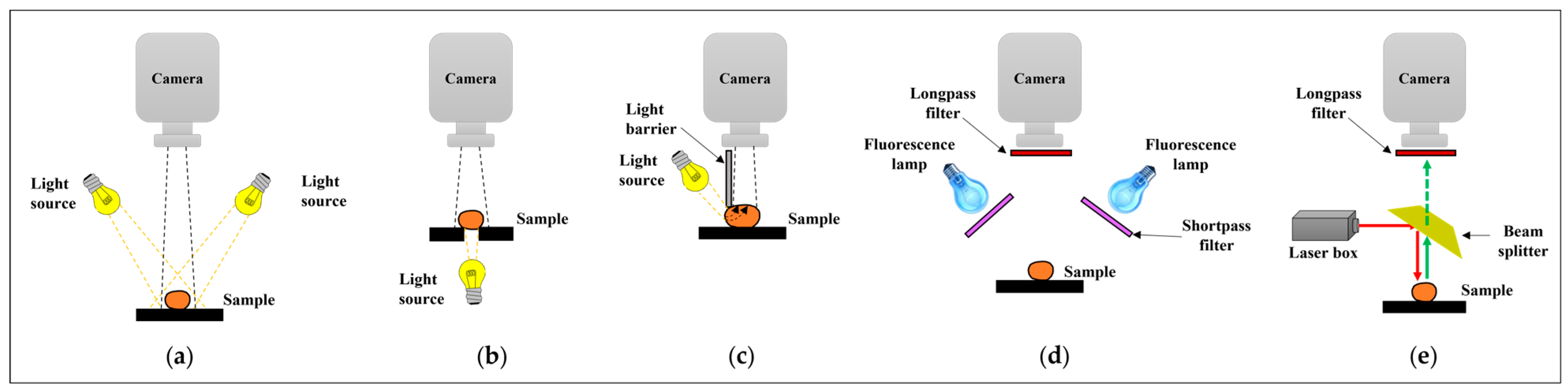
| Sensing Mode | Description |
|---|---|
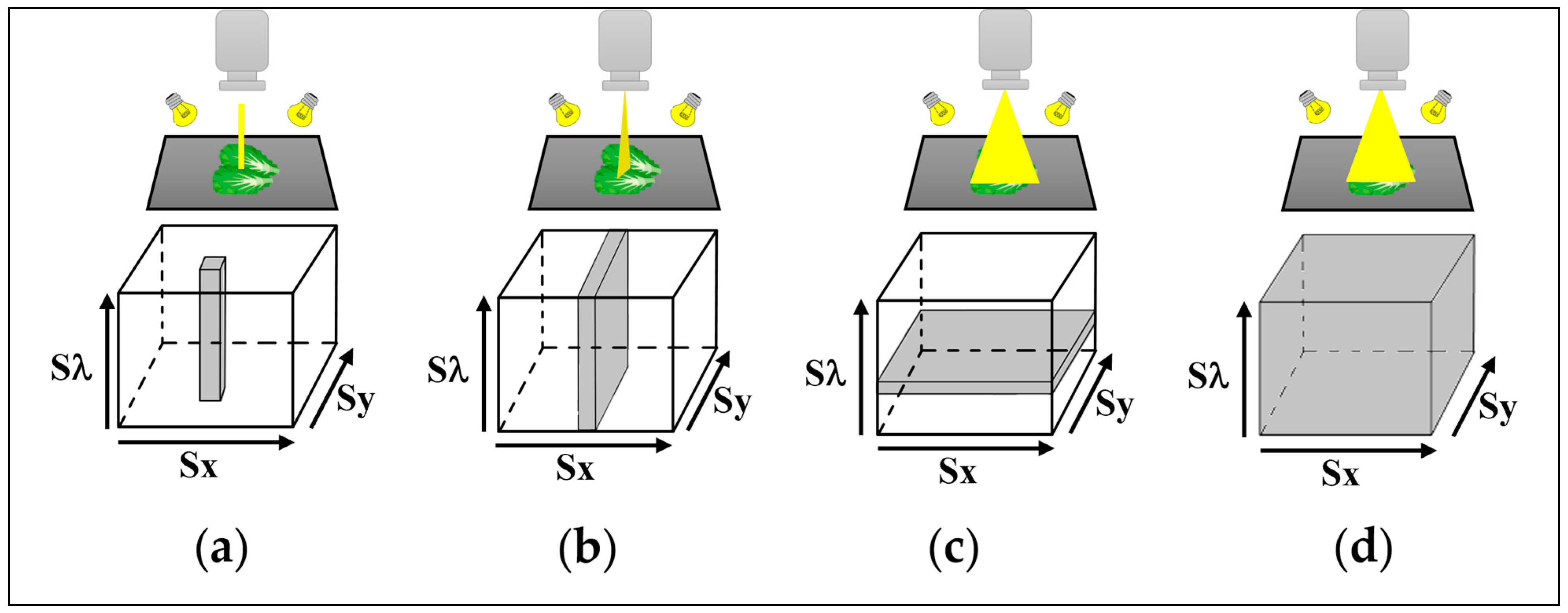
| Diffuse reflectance (Figure 2a) | The detector and the light source are generally positioned above the sample, and the reflected light from the illuminated area is acquired by the detector. This mode is applied to evaluate external quality properties, such as size, shape, color, surface texture, and physical defects. |
| Transmittance (Figure 2b) | The sample is placed between the detector and light source, and the radiation which crosses over it is measured. This method is generally used to evaluate internal quality features such as internal defects or chemical compound concentration. However, the sample thickness has an impact on the signal, which decreases as thickness increases. |
| Interactance (Figure 2c) | The imaging area is isolated from the light source by a predetermined angle or distance. The measured light passes through a little layer of tissue beneath the surface. Thus, it is possible to obtain more information from the inside of the sample than with the reflectance mode. |
| Fluorescence (Figure 2d) | It measures the radiation emitted by the sample after excitation by absorbing light radiation at a high energy level. The emission is in two main spectral ranges, from blue to green (450–550 nm) and from red to far red (690–740 nm), and it is characterized by three peaks in the blue, red, and far-red bands. In fluorescence imaging, the light source and the detector are positioned at the same side of the sample. Generally, the light excitation sources used are Xenon arc lamps, lasers, or LEDs. |
| Raman scattering (Figure 2e) | It requires a block of the excitation light from the detection end and an intense excitation light source coupled with a high-performance detector to ensure adequate signal quality. The excitation is typically performed with diode lasers at 785 or 830 nm. As the Raman signals are very weak, commercial Raman imaging systems typically have small imaging areas at the millimeter scales or less (for microscopic applications). |
| Qualitative Features | Description | ||
|---|---|---|---|
| External features | Color | First element of quality monitoring and conveys consumer choice. It is an indirect indicator of features like freshness, desirability and variety, maturity, and safety, which are related to the physical, chemical, or microbial changes that occur in ripeness and the postharvest processing and handling stages [65]. | |
| Defects | Surface defects | Mainly due to mechanical injuries, insects, diseases, and over- or under-ripeness. Damaged products should be selected and removed, during postharvest processing, to reduce losses by avoiding secondary contaminations [66]. | |
| Physiological disorders | Appear during postharvest after internal or external stresses, like nutritional deficiency, senescence, suppressed respiration, and extreme temperature [2]. | ||
| Chilling injury | Caused mainly by postharvest storing at low temperatures which produces internal browning, deteriorated texture, juiciness deficiency, and unpleasantness [64]. | ||
| Internal features | Texture | Capacity to withstand deformation actions like biting, chewing, and grinding, with an impact on food acceptability and consumer preferences [64]. Firmness is an indicator of the maturity stage and shelf life. Firmness loss in fruits is primarily caused by the enzymatic degradation of pectin present in the intercellular space and cell wall [62]. | |
| Nutritional value | Represented by the caloric intake or elements that are important from a nutritional point of view. | ||
| Safety | Absence of antinutritional substances | e.g., nitrates and nitrites, pesticide residues, insect or pest infestation, fecal contamination, naturally occurring undesirable compounds, and plant growth regulators [2,67]. | |
| Absence of pathogenic microorganisms | e.g., Escherichia coli, Salmonella spp., and Listeria monocytogenes whose presence is caused by soil or manure contamination, irrigation water, inappropriate packaging, and inadequate storage temperatures [68]. | ||
Disclaimer/Publisher’s Note: The statements, opinions and data contained in all publications are solely those of the individual author(s) and contributor(s) and not of MDPI and/or the editor(s). MDPI and/or the editor(s) disclaim responsibility for any injury to people or property resulting from any ideas, methods, instructions or products referred to in the content. |
© 2023 by the authors. Licensee MDPI, Basel, Switzerland. This article is an open access article distributed under the terms and conditions of the Creative Commons Attribution (CC BY) license (https://creativecommons.org/licenses/by/4.0/).
Share and Cite
Vignati, S.; Tugnolo, A.; Giovenzana, V.; Pampuri, A.; Casson, A.; Guidetti, R.; Beghi, R. Hyperspectral Imaging for Fresh-Cut Fruit and Vegetable Quality Assessment: Basic Concepts and Applications. Appl. Sci. 2023, 13, 9740. https://doi.org/10.3390/app13179740
Vignati S, Tugnolo A, Giovenzana V, Pampuri A, Casson A, Guidetti R, Beghi R. Hyperspectral Imaging for Fresh-Cut Fruit and Vegetable Quality Assessment: Basic Concepts and Applications. Applied Sciences. 2023; 13(17):9740. https://doi.org/10.3390/app13179740
Chicago/Turabian StyleVignati, Sara, Alessio Tugnolo, Valentina Giovenzana, Alessia Pampuri, Andrea Casson, Riccardo Guidetti, and Roberto Beghi. 2023. "Hyperspectral Imaging for Fresh-Cut Fruit and Vegetable Quality Assessment: Basic Concepts and Applications" Applied Sciences 13, no. 17: 9740. https://doi.org/10.3390/app13179740
APA StyleVignati, S., Tugnolo, A., Giovenzana, V., Pampuri, A., Casson, A., Guidetti, R., & Beghi, R. (2023). Hyperspectral Imaging for Fresh-Cut Fruit and Vegetable Quality Assessment: Basic Concepts and Applications. Applied Sciences, 13(17), 9740. https://doi.org/10.3390/app13179740