Abstract
A tailing storage facility (TSF) is a complex hydrotechnical structure that requires continuous monitoring to prevent catastrophic dam damage. One critical issue to control is the soil’s characteristics, which is why many field and laboratory tests are carried out on the dam to determine the relevant soil parameters. Among these tests, down-hole seismic tests, such as SCPT, are performed to determine, e.g., the shear wave velocity. However, accurately calculating the difference in the times of the arrival of the wave at the two geophones is crucial to determining its value. This article proposes a novel method for estimating this variable using the DTW (Dynamic Time Warping) algorithm, which calculates the shift between two signals by determining their optimal match. The article also addresses signal interference and proposes methods for clearing it to obtain more accurate results. Furthermore, the article introduces a method for measuring the signals’ quality based on their similarity, which helps assess whether determining the shear wave velocity is possible for a given sample.
1. Introduction
In the mining industry, the storage of post-flotation waste represents one of the final stages of the production process. This stage is of critical importance given the substantial volume of waste generated, which typically constitutes the majority of the extracted ore. To store the waste, tailing storage facilities (TSFs) are used, which are large, complex hydrotechnical structures where waste is deposited through hydrotransportation. Given the nature of tailings and the structure of reservoirs, the continuous monitoring of the dam’s stability is required. This need for monitoring has been further highlighted by the occurrence of numerous TSF disasters, which pose a significant threat to the environment and human life [1,2]. The main causes of TSF failures include the instability of the dam slope, earthquake load, overtopping, seepage, and unsuitable foundations [3,4]. Monitoring a TSF requires numerous tests, both in the laboratory and in the field. Although most of the tests, particularly those that are minimally invasive, do not directly provide the sought-after information, they do yield indirect parameters that require careful analysis and interpretation. One parameter of particular importance is the shear wave velocity (v), which represents a fundamental soil mechanical property. Along with other measurements, this feature can be applied to evaluate soil characteristics. The primary parameter obtained through studying shear wave velocity is used to measure material stiffness, specifically the dynamic elastic shear modulus, which is defined as
where is the soil density [5]. This parameter holds significant importance in earthquake ground reaction analysis because the stiffness of the material affects the way the soil reacts to seismic vibrations and the distribution of stresses and strains in the soil. Correlating wave velocity with measurements from other tests may provide opportunities to extend or replace some of these tests. This dependence can be examined for, among others, the cone penetration resistance from a CPT, the standard penetration test blow count from an SPT, as well as the effective confining pressure and void ratio from laboratory tests [6]. The benefit of shear wave velocity application in the case of TSF is the ability to use the parameter to assess the seismic resistance of soil to liquefaction [7], which is one of the causes of TSF failures. The speed of the shear wave can be determined through various tests. The two basic tests are the cross-hole test and the down-hole test. Both of these tests are based on the induction of a seismic shear wave that is received by a geophone placed on a probe inserted into the soil. The main difference between these tests is the location of the source of the wave. With the cross-hole method, the source is placed in a second borehole at the same height as the geophone.
Due to this, it is only necessary to determine the time of arrival of the wave to the geophone. The ratio of the constant distance between the source and the receiver and the determined time difference enables the calculation of the wave speed. Down-hole test results, where the source is on the surface and is received by two geophones placed at different depths on the probe, are slightly more challenging to interpret. In this case, the crucial task is to determine the difference in the times of the arrival of the wave at both geophones (Δt). The constant difference between the localization of the geophones makes it possible to indicate the wave speed at individual depths. In order to determine Δt, it is necessary to correlate both signals and determine the value of the shift between them. One common method of Δt determination is the cross-correlation method, which is described in more detail in [8]. However, the task can be especially difficult when the signals are noisy or have other irregularities. For this reason, it is necessary to develop an accurate method of determining the value of the shift as well as defining the accuracy of the result obtained. The advantages of the down-hole method over the cross-hole method are that it is less invasive, as it involves making only one well, and it is possible by performing the seismic cone penetration test (SCPT).
Our study introduces a novel method for determining the time delay of shear wave arrival using Dynamic Time Warping (DTW), a signal similarity algorithm, to determine the shear wave velocity. This method emphasizes the importance of proper signal preconditioning techniques, such as noise removal, amplitude normalization, trend removal, and the extraction of the informational fragment of the signal. Moreover, a signal quality assessment method based on signal similarity was proposed using the DTW algorithm. The study concludes with a presentation of results that demonstrate the accuracy of the proposed method and the significance of signal quality assessment.
2. Investigated Object
The work was carried out as part of the SEC4TD project [9], which focused on building an IoT platform for managing the safety of tailings dams. One of the key use cases is the Gilów Tailings Storage Facility (TSF). The Gilów TSF, which is a man-made reservoir located in the Lower Silesian Voivodeship of southwest Poland, was primarily used for storing post-flotation waste generated in the nearby Lubin copper mine. The construction of this reservoir was initiated in 1968 and completed by the late 1960s. The maximum capacity of the reservoir was achieved in June 1980, when it reached an elevation of 177.5 m above sea level, after receiving around 60 million cubic meters of tailings during its operational period.
The Gilów TSF (see Figure 1) was decommissioned in 1977, and the process of afforestation is currently under way. In the years 1982–1986, the area was subjected to extensive biological reclamation works aimed at the ecological restoration of the land. Since May 1990, it has been utilized as an emergency retention reservoir for Żelazny Most [10], with water being directed for industrial purposes through the overflow tower.
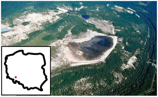
Figure 1.
Closed Gilów TSF from a bird’s-eye view and approximate location (red point).
3. Data Preparation
The shear wave arrives first at the upper geophone and later at the lower geophone (Δt). Due to depth deference, the amplitudes are different, and both measurements are often noisy or contain irregularities from various origins. To utilize the DTW method for comparing the waves recorded using two geophones, it is imperative to effectively eliminate any irregularities and phenomena that may cause inaccurate matching. It is necessary to avoid cases where the algorithm will try to find a relationship between incorrect values in the signals, including noise.
The most informative fragment (the shadowed part in Figure 2) to be compared in order to find the arrival time difference is the moment of the appearance of the greatest amplitude to the vanishing of the signal. The remaining fragments mainly contain noise, which is not relevant for analysis. The same wave recorded using upper and lower geophones may have a different noise appearance; it has been observed that more in-depth measurements have more noticeable noise. Furthermore, it has been observed that the noise present in the signal prior to the arrival of the wave may exhibit a different character than it does at the time of the wave’s appearance. Consequently, the signal decomposition method was deemed unsuitable, and simple smoothing techniques were employed to mitigate the noise.
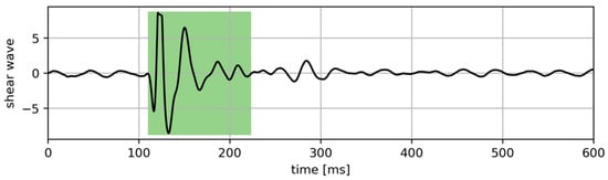
Figure 2.
An example of a signal measured using one geophone. The shadowed part is the most informative part.
Another anomaly detected in the signals is the occurrence of a trend or the signal shift by a constant value. The wave should ideally oscillate around zero, and any trend or shift is considered abnormal and may result in measurement errors. To address this, a linear trend was fitted to the signal in each case and removed.
Another phenomenon that can impact signal comparison is varying amplitude values. While they are not data errors, comparing two signals with differing amplitudes can lead to inaccurate outcomes. Thus, the decision was made to normalize the compared wave values with respect to their amplitudes. Additionally, extracting the most informative segment from the signal is a crucial step toward improving the quality of the results. Geophone signal registration occurs over a fixed duration, including the period before wave arrival, the moment of peak amplitude, and the damped wave signal.
Taking into account all the above factors, the following methods of preparing shear wave data are proposed.
- The smoothing of the s signal value in order to minimize the noise was performed using a simple moving average in a window of 10 samples (2 ms);
- The removal of the linear trend selected using the least squares method;
- The normalization of signals recorded using both geophones and in terms of amplitude;where .
- The isolation of the information part of the signal s.
- The determination of the signal envelope relative to the quantiles counted in the window of 100 samples: is the lower envelope, and is the upper envelope.
- The determination of moving average values in a window of 100 samples for positive signal values and negative signal values .
- The informative value range is determined as follows:
The most informative part starts with the appearance of the greatest amplitude and ends with the vanishing of the signal. The starting point is the first index, where the upper envelope is greater than the moving average from positive signal values, and the lower envelope is lower than the moving average from negative signal values.
- d.
- After determining the informative interval for the signal registered using the first geophone and the second one , both signals are limited to one interval being their sum:
The period of time used in the simple moving average method and the size of the window used to calculate the signal envelope were experimentally chosen.
4. Methodology
4.1. DTW
Dynamic Time Warping (DTW) is a well-known method of assessing the similarity between two signals or time series. DTW, in contrast to the simple Euclidean distance measure, is resistant to signal shifts in time and their stretching or shortening. It gives the opportunity to compare each pair of values of both signals in order to find the best match with respect to the smallest distance [11].
Assuming two signals, of length n and of length m are given as
it is possible to compare each value of with using a chosen distance function, for example,
The results of the above function can be presented in the form of a two-dimensional n-by-m matrix. An example of such a comparison of two signals is shown in Figure 3, where the distance values are marked against a color scale. The task of DTW is to indicate the so-called warping path (W), i.e., a sequence of points, so as to minimize the distance between the A and B values. It can be defined as
where corresponds to the point . The optimal warping path is the one for which the sum of the distances between the values along the path is the smallest. It is also the best match between the A and B signals. Thus, the DTW measure can be defined as follows [11]:
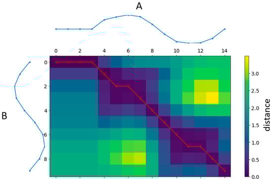
Figure 3.
An example of visualizing the result of the DTW algorithm for A and B signals marked with blue curves. The red curve is the optimal warping path.
In Figure 3, the optimal warping path is marked with a red line.
The Dynamic Time Warping (DTW) method is widely used in various fields, particularly in situations where it is necessary to compare signals of varying lengths that may contain the shifting, stretching, or shortening of individual fragments.
A particularly relevant topic is the recognition of patterns or motifs in signals [12]. The first instance in which the DTW algorithm was used was for the recognition of human speech [13,14,15,16]. Speech recognition requires finding patterns of individual words in a sound record, which can be uttered at different speeds by different people, which the DTW method is resistant to. This topic is still being developed, and more and more accurate methods using DTW in combination with other techniques are being developed. DTW has been combined with Mel-Frequency Cepstral Coefficients (MFCC) in several studies, including [17,18], to effectively recognize patterns in human speech signals. In [19], a solution is proposed that combines DTW with a Support Vector Machine, while in [20,21], DTW is combined with a Hidden Markov Model. In addition to recognizing human speech, it is also possible to apply DTW to recognize environmental sounds [22], such as bird calls [23]. Some other applications of DTW for pattern recognition include the recognition of gestures from inertial data [24,25,26], sign language [27], human movement from movies [28,29,30], as well as applications in medicine, such as the classification of heart sounds [31,32] or ECG arrhythmias [33,34]. In the case of machines, DTW can be used in the context of diagnostics of, for example, motor drives [35] or location from inertial data [36], as well as data reduction generated in autonomous driving systems [37]. The DTW method can also be extended to more dimensions. Two methods, dependent and independent ones, are used for this, which give different results, and the choice is not obvious [38]. Pattern recognition can also be used as a means to find the offset of one signal relative to another, as presented in this paper.
4.2. Signal Quality Assessment
Despite the adequate preconditioning of signals, it has been found that some of them are still of a poor quality, which makes it impossible to determine the difference in the wave arrival times or makes the results less reliable. Poor-quality signals have high-level signal noise, a lack of a characteristic maximum amplitude, as well as other qualities that make one of the waves not similar to the other from the same sample. For this reason, it was decided to test the quality based on the similarity of the waves recorded using both geophones. Both signals are expected to have similar shapes, but differ in their timing. Significant deviations in the waveform shape could indicate the presence of disturbances, which may compromise the ability to compare the signals and ascertain differences in the wave arrival times. The similarity between the signals was measured using the Dynamic Time Warping (DTW) distance measure, where a greater similarity indicates the better quality and higher accuracy of the final result. To standardize the DTW measure across signals of varying lengths, the distance value was divided by the measurement length . Additionally, in order to normalize the measures of all the results, the value was divided by the maximum value occurring in all the analyzed cases (). Considering the above, the following measure of the quality of signals is proposed in relation to their similarity:
An example of the determined quality values for the left shear wave and right shear wave depending on their depth is presented in Figure 4. The quality is also illustrated with the proposed color scale, which is used in the next part to compare the results of the estimated wave speed with the quality of the signals.
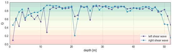
Figure 4.
An example of signal quality comparison based on depth measurements of left and right shear waves (the color scale in the background also corresponds to the quality values).
4.3. Determination of the Wave Speed
The speed of the wave relative to the height can be determined based on the difference in the arrival times of the wave at both geophones (). In practice, it means finding the shift value between two waves in the time domain. The DTW method is mainly used to determine the similarity between signals, and it also plays this role in the analysis of signal quality discussed in the Section 4.2. However, the assumption of the method of matching signals with the possibility of shifts in time also makes it achievable to determine the value of this shift for each signal value. Ideally, this shift should be constant for each value. In practice, however, the signals will never be identical, and the DTW algorithm will try to match them as much as possible using different shift values. Therefore, it is necessary to establish a standard for determining the primary shift, and it seems most intuitive to use the median value, which is the most frequently occurring value. It was assumed that is the shear wave recorded using the first geophone and is the shear wave recorded using the second geophone, where the distance from the wave source to the first geophone is greater than the distance to the second one. Using the DTW algorithm, the optimal match of to was determined, obtaining a path , where is a vector of index numbers for the signal , and is a vector of index numbers for . Thus, the shifts between the values of the signals (in the case of optimal matching) are equal:
This vector, based on the assumption about the distance of the geophones from the wave source, should take positive values (the signal will reach the first geophone later). However, due to real, non-ideal conditions, negative values may also appear in the result, which are certainly not related to the real difference in the arrival times of the wave. For this reason, it was decided to exclude them from the analysis:
The main signal shift was determined by the median . Knowing that the measurements are made with a frequency of 0.2 ms, it can be defined as
The distance d between the geophones is fixed (0.5 or 1 m depending on SCPT cone model); therefore, the speed of the wave can be determined by
An example of a shear wave recorded using both geophones is shown in Figure 5a. The signals, in this case, are of a good quality; . The result of shifting the wave recorded using the second geophone by the value determined by employing the proposed method is shown in Figure 5b. There is a clear coincidence of both waves, which means that the shift value was correctly determined.
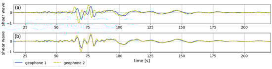
Figure 5.
Examples of a selected shear wave recorded using two geophones (a), and after shifting by the determined value Δt, the wave recorded using geophone 2 (b).
5. Results
The proposed method of determining the wave speed was tested on real measurements from three SCPT tests carried out on the tailing storage facility dam. Each of the tests was carried out at a depth of about 50 m, and down-hole measurements were performed every 1 m by generating a wave from the left and right sides. This resulted in a total of almost 300 recorded signals (each using two geophones). Cross-hole tests were carried out at the same measurement points, which provide reliable information about the wave speed (later referred to as “real” information). These measurements were used as reference values to assess the accuracy of the estimated results of the DTW-based method. Each of the waves was also assessed in terms of signal quality according to the method of examining the similarity of signals using DTW. Figure 6 shows the results obtained for three tests (Figure 6a–c). The estimated wave speed is presented in relation to the measurement depth and compared with the actual value. In addition, the quality (Q) is marked in color, where red means a signal quality close to 0 and green means a signal quality close to 1. It can be seen that the estimated values are close to the real ones, but they do not fully coincide. There are also some large deviations that usually correlate with a poor signal quality. The worst results were obtained for measurement no. three, which is the left wave.
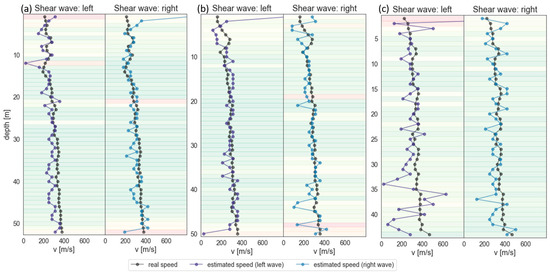
Figure 6.
Comparison of the estimated wave speed determined by the DTW-based method with the actual values from cross-hole tests for three SCPT studies (a–c). The color scale from red to green indicates the quality of the signals (red—low quality, green—high quality).
The obtained wave speed estimation results were also compared using the RMSE measure, where the cross-hole test result was taken as the actual value (Table 1). The value was determined each time for all the waves and after rejecting those of a low quality ( and ). Assuming that the quality threshold is set to be greater than 0.5, approximately 9% of the measurements are excluded on average. Raising the quality threshold to be greater than 0.7 results in the rejection of approximately 25% of signals from the analysis. However, it can be seen that the introduction of these restrictions increases the accuracy of the results. After the introduction of the first quality constraint, the RMSE was lower by an average of 37%. Increasing the constraint to no longer improves the accuracy of the result as much, so it may be unnecessary.

Table 1.
Comparison of RMSE values for individual tests.
The results show that, in addition to using a good method for determining the difference in the time of arrival of the wave, it is also very important to evaluate the quality of the measurements in order to avoid erroneous results. Furthermore, having two measurements (left shear wave and right shear wave) and a quality assessment means that the result of a higher-quality measurement can be taken as the final value of the estimated speed.
As mentioned in the Introduction, a common way of finding Δt is using the cross-correlation method. The disadvantage is that the precision is limited by the signal resolution. Moreover, in more difficult cases, i.e., measurements close to the surface or the deepest ones, the cross-correlation method gave unrealistic results because the shear wave speed was too high [8]. Both methods were tested on the same dataset. The advantages of using the DTW method are its efficacy (i.e., more realistic results in difficult cases) and the precision of the shear wave speed.
6. Discussion
The results show that the determination of the difference in the times of arrival of a wave at two geophones during a down-hole test is possible using the DTW method. However, the proper preconditioning of seismic signals is necessary before attempting to match them. For this reason, a comprehensive data preparation procedure is proposed that includes noise and trend removal, amplitude normalization, and the extraction of the informative part of the signal. Such data cleaning allows more accurate results to be obtained. Despite the appropriate preparation of signals, some of them still exhibit a low quality, which renders further analysis unfeasible. It is suggested that the signals’ quality should be evaluated based on their similarity. Only highly similar signals can enable the precise determination of wave arrival time differences. Due to the possible shifts, extensions, or contractions in the signals, the DTW algorithm is used in this regard.
The proposed methods were tested on real data, and the estimated speed values were compared with the speed determined from the cross-hole test, which served as reference data. The results showed a large influence of signal quality on the accuracy of the results. Removing about 9% of very low-quality data reduced the RMSE by an average of 37%. The proposed method of determining the signal quality may also allow researchers to select a more precise result obtained from left and right shear wave measurements, as well as the ability to repeat the test in the same place.
Author Contributions
Conceptualization, P.S. (Paweł Stefaniak) and N.D.-M.; methodology, N.D.-M., W.K., M.S. and P.S. (Paweł Stefaniak); software, N.D.-M. and W.K.; validation, W.K., M.S. and S.A.; formal analysis, W.K. and M.S.; investigation, P.S. (Paweł Stefaniak) and P.S. (Paweł Stefanek); resources, N.D.-M. and S.A.; data curation, W.K.; writing—original draft preparation, N.D.-M., W.K.; writing—review and editing, P.S. (Paweł Stefaniak); visualization, N.D.-M. and W.K.; supervision, S.A., P.S. (Paweł Stefaniak) and P.S. (Paweł Stefanek); project administration, S.A. and P.S. (Paweł Stefaniak); funding acquisition, S.A. and P.S. (Paweł Stefaniak). All authors have read and agreed to the published version of the manuscript.
Funding
This work has received funding from EIT RawMaterials GmbH under Framework Partnership Agreement No 21123 (project Sec4TD).
Institutional Review Board Statement
Not applicable.
Informed Consent Statement
Not applicable.
Data Availability Statement
Data supporting this study cannot be made available due to nature of the research.
Conflicts of Interest
The authors declare no conflict of interest.
References
- Koperska, W.; Stachowiak, M.; Duda-Mróz, N.; Stefaniak, P.; Jachnik, B.; Bursa, B.; Stefanek, P. The Tailings Storage Facility (TSF) stability monitoring system using advanced big data analytics on the example of the Żelazny Most Facility. Arch. Civ. Eng. 2022, 68, 297–311. [Google Scholar]
- Fuławka, K.; Pytel, W.; Pałac-Walko, B. Near-Field Measurement of Six Degrees of Freedom Mining-Induced Tremors in Lower Silesian Copper Basin. Sensors 2020, 20, 6801. [Google Scholar] [CrossRef] [PubMed]
- Clarkson, L.; Williams, D. Critical review of tailings dam monitoring best practice. Int. J. Min. Reclam. Environ. 2020, 34, 119–148. [Google Scholar] [CrossRef]
- Fuławka, K.; Kwietniak, A.; Lay, V.; Jaśkiewicz-Proć, I. Importance of seismic wave frequency in FEM-based dynamic stress and displacement calculations of the earth slope. Stud. Geotech. Mech. 2022, 44, 82–96. [Google Scholar] [CrossRef]
- Robertson, P.K.; Campanella, R.G.; Gillespie, D.; Rice, A. Seismic Cpt to Measure in Situ Shear Wave Velocity. J. Geotech. Eng. 1986, 112, 791–803. [Google Scholar] [CrossRef]
- Hussien, M.N.; Karray, M. Shear wave velocity as a geotechnical parameter: An overview. Can. Geotech. J. 2015, 53, 252–272. [Google Scholar] [CrossRef]
- Kayen, R.; Moss, R.E.S.; Thompson, E.M.; Seed, R.B.; Cetin, K.O.; Der Kiureghian, A.; Tanaka, Y.; Tokimatsu, K. Shear-Wave Velocity–Based Probabilistic and Deterministic Assessment of Seismic Soil Liquefaction Potential. J. Geotech. Geoenviron. Eng. 2013, 139, 407–419. [Google Scholar] [CrossRef]
- Duda, N.; Jachnik, B.; Stefaniak, P.; Bursa, B.; Stefanek, P. Tailings Storage Facility stability monitoring using CPT data analytics on the Zelazny Most facility. In Proceedings of the 40th Application of Computer and Operation Research (APCOM) 2021—Minerals Industry 4.0: The Next Digital Transformation in Mining, Johannesburg, South Africa, 29 August–1 September 2021. [Google Scholar]
- SEC4TD—Securing Tailings Dam Infrastructure with an Innovative Monitoring System. Available online: https://sec4td.fbk.eu/ (accessed on 10 July 2023).
- Koperska, W.; Stachowiak, M.; Jachnik, B.; Stefaniak, P.; Bursa, B.; Stefanek, P. Machine Learning Methods in the Inclinometers Readings Anomaly Detection Issue on the Example of Tailings Storage Facility. In IFIP International Workshop on Artificial Intelligence for Knowledge Management; Springer: Cham, Switzerland, 2021; pp. 235–249. [Google Scholar] [CrossRef]
- Berndt, D.J.; Clifford, J. Using dynamic time warping to find patterns in time series. In Proceedings of the 3rd International conference on Knowledge Discovery and Data Mining, Seattle, WA, USA, 31 July–4 August 1994; Volume 10, pp. 359–370. [Google Scholar]
- Mueen, A. Time series motif discovery: Dimensions and applications. Wiley Interdiscip. Rev. Data Min. Knowl. Discov. 2014, 4, 152–159. [Google Scholar] [CrossRef]
- Vintsyuk, T.K. Speech discrimination by dynamic programming. Cybern. Syst. Anal. 1968, 4, 52–57. [Google Scholar] [CrossRef]
- Sakoe, H.; Chiba, S. Dynamic programming algorithm optimization for spoken word recognition. IEEE Trans. Acoust. Speech Signal Process. 1978, 26, 43–49. [Google Scholar] [CrossRef]
- Myers, C.; Rabiner, L.; Rosenberg, A. Performance tradeoffs in dynamic time warping algorithms for isolated word recognition. IEEE Trans. Acoust. Speech Signal Process. 1980, 28, 623–635. [Google Scholar] [CrossRef]
- Juang, B.-H. On the Hidden Markov Model and Dynamic Time Warping for Speech Recognition—A Unified View. ATT Bell Lab. Tech. J. 1984, 63, 1213–1243. [Google Scholar] [CrossRef]
- Mohan, B.J. Speech recognition using MFCC and DTW. In Proceedings of the 2014 International Conference on Advances in Electrical Engineering (ICAEE), Vellore, India, 9–11 January 2014; pp. 1–4. [Google Scholar]
- Dhingra, S.D.; Nijhawan, G.; Pandit, P. Isolated speech recognition using MFCC and DTW. Int. J. Adv. Res. Electr. Electron. Instrum. Eng. 2013, 2, 4085–4092. [Google Scholar]
- Ismail, A.; Abdlerazek, S.; El-Henawy, I.M. Development of Smart Healthcare System Based on Speech Recognition Using Support Vector Machine and Dynamic Time Warping. Sustainability 2020, 12, 2403. [Google Scholar] [CrossRef]
- De Wachter, M.; Matton, M.; Demuynck, K.; Wambacq, P.; Cools, R.; Van Compernolle, D. Template-Based Continuous Speech Recognition. IEEE Trans. Audio Speech Lang. Process. 2007, 15, 1377–1390. [Google Scholar] [CrossRef]
- Ravinder, K. Comparison of hmm and dtw for isolated word recognition system of punjabi language. In Iberoamerican Congress on Pattern Recognition; Springer: Berlin/Heidelberg, Germany, 2010; pp. 244–252. [Google Scholar]
- Cowling, M.; Sitte, R. Comparison of techniques for environmental sound recognition. Pattern Recognit. Lett. 2003, 24, 2895–2907. [Google Scholar] [CrossRef]
- Kogan, J.A.; Margoliash, D. Automated recognition of bird song elements from continuous recordings using dynamic time warping and hidden Markov models: A comparative study. J. Acoust. Soc. Am. 1998, 103, 2185–2196. [Google Scholar] [CrossRef]
- Hartmann, B.; Link, N. Gesture recognition with inertial sensors and optimized DTW prototypes. In Proceedings of the 2010 IEEE International Conference on Systems, Man and Cybernetics, Istanbul, Turkey, 10–13 October 2010; pp. 2102–2109. [Google Scholar]
- Hussain, S.M.A.; Rashid, A.B.M.H.-U. User independent hand gesture recognition by accelerated DTW. In Proceedings of the 2012 International Conference on Informatics, Electronics & Vision (ICIEV), Dhaka, Bangladesh, 18–19 May 2012; pp. 1033–1037. [Google Scholar]
- Carmona, J.M.; Climent, J. A performance evaluation of HMM and DTW for gesture recognition. In Iberoamerican Congress on Pattern Recognition; Springer: Berlin/Heidelberg, Germany, 2012; pp. 236–243. [Google Scholar]
- Lichtenauer, J.F.; Hendriks, E.A.; Reinders, M.J. Sign Language Recognition by Combining Statistical DTW and Independent Classification. IEEE Trans. Pattern Anal. Mach. Intell. 2008, 30, 2040–2046. [Google Scholar] [CrossRef]
- Blackburn, J.; Ribeiro, E. Human Motion Recognition Using Isomap and Dynamic Time Warping. In Human Motion–Understanding, Modeling, Capture and Animation; Springer: Berlin/Heidelberg, Germany, 2007; pp. 285–298. [Google Scholar] [CrossRef]
- Okada, S.; Hasegawa, O. Motion recognition based on dynamic-time warping method with self-organizing incremental neural network. In Proceedings of the 2008 19th International Conference on Pattern Recognition, Tampa, FL, USA, 8–11 December 2008; pp. 1–4. [Google Scholar] [CrossRef]
- Rybarczyk, Y.; Deters, J.K.; Gonzalo, A.A.; Esparza, D.; Gonzalez, M.; Villarreal, S.; Nunes, I.L. Recognition of Physiotherapeutic Exercises Through DTW and Low-Cost Vision-Based Motion Capture. In Advances in Human Factors and Systems Interaction, Proceedings of the AHFE 2017 International Conference on Human Factors and Systems Interaction, Los Angeles, CA, USA, 17−21 July 2017; Springer: Cham, Switzerland, 2018; pp. 348–360. [Google Scholar] [CrossRef]
- Fu, W.; Yang, X.; Wang, Y. Heart sound diagnosis based on DTW and MFCC. In Proceedings of the 2010 3rd International Congress on Image and Signal Processing, Yantai, China, 16–18 October 2010; Volume 6, pp. 2920–2923. [Google Scholar]
- Ortiz, J.J.G.; Phoo, C.P.; Wiens, J. Heart sound classification based on temporal alignment techniques. In Proceedings of the 2016 Computing in Cardiology Conference, Vancouver, BC, Canada, 11–14 September 2016; pp. 589–592. [Google Scholar]
- Huang, B.; Kinsner, W. ECG frame classification using dynamic time warping. In Proceedings of the IEEE CCECE2002 Canadian Conference on Electrical and Computer Engineering, Conference Proceedings (Cat. No. 02CH37373), Winnipeg, MB, Canada, 12–15 May 2002; Volume 2, pp. 1105–1110. [Google Scholar]
- Tuzcu, V.; Nas, S. Dynamic Time Warping as a Novel Tool in Pattern Recognition of ECG Changes in Heart Rhythm Disturbances. In Proceedings of the 2005 IEEE International Conference on Systems, Man and Cybernetics, Waikoloa, HI, USA, 12 October 2005; Volume 1, pp. 182–186. [Google Scholar] [CrossRef]
- Zhen, D.; Wang, T.; Gu, F.; Ball, A. Fault diagnosis of motor drives using stator current signal analysis based on dynamic time warping. Mech. Syst. Signal Process. 2013, 34, 191–202. [Google Scholar] [CrossRef]
- Stefaniak, P.; Jachnik, B.; Koperska, W.; Skoczylas, A. Localization of LHD Machines in Underground Conditions Using IMU Sensors and DTW Algorithm. Appl. Sci. 2021, 11, 6751. [Google Scholar] [CrossRef]
- Gao, Z.; Yu, T.; Sun, T.; Zhao, H. Data Filtering Method for Intelligent Vehicle Shared Autonomy Based on a Dynamic Time Warping Algorithm. Sensors 2022, 22, 9436. [Google Scholar] [CrossRef] [PubMed]
- Shokoohi-Yekta, M.; Hu, B.; Jin, H.; Wang, J.; Keogh, E. Generalizing DTW to the multi-dimensional case requires an adaptive approach. Data Min. Knowl. Discov. 2017, 31, 1–31. [Google Scholar] [CrossRef] [PubMed]
Disclaimer/Publisher’s Note: The statements, opinions and data contained in all publications are solely those of the individual author(s) and contributor(s) and not of MDPI and/or the editor(s). MDPI and/or the editor(s) disclaim responsibility for any injury to people or property resulting from any ideas, methods, instructions or products referred to in the content. |
© 2023 by the authors. Licensee MDPI, Basel, Switzerland. This article is an open access article distributed under the terms and conditions of the Creative Commons Attribution (CC BY) license (https://creativecommons.org/licenses/by/4.0/).