Analysis of Carbon Emissions in Heterogeneous Traffic Flow within the Influence Area of Highway Off-Ramps

Abstract

With the continuous advancements in electrification, connectivity, and intelligence in the automotive industry, the mixed traffic of vehicles with different levels of driving automation is changing the carbon emission characteristics in the impact areas of off-ramps on highways. Considering the insufficient research on the carbon emission characteristics of heterogeneous traffic flow in the downstream influence areas of highway off-ramps, this study applied a scenario analysis method. Furthermore, considering factors such as vehicle composition, road control, and platoon management, it establishes and calibrates measurement models for carbon emissions from conventional vehicles, intelligent vehicles, the platoon driving of electric vehicles, and the mixed platoon driving of conventional vehicles and electric vehicles. This study also provides a simulation scenario for a three-lane highway off-ramp based on the actual conditions of the Xi’an Ring Expressway. Finally, by applying the constructed carbon emission calculation models for heterogeneous traffic flow in the intelligent vehicle mixed traffic scenario, a quantitative analysis was conducted to assess the impacts of the intelligent vehicle infiltration rate, off-ramp vehicle proportion, smart-vehicle-dedicated lanes, and platoon driving on carbon emissions in the downstream influence area of off-ramps. The results revealed the impact of intelligent vehicle integration and platoon driving on carbon emission characteristics in the downstream influence areas of highway off-ramps.

1. Introduction

Carbon emissions have become an important topic of discussion in recent years, and transportation carbon emissions, as an important component of carbon emissions, have also received widespread attention [1]. Along with the innovation in driving automation systems, the innovation and development of automobile industry technology are of great significance for reducing energy consumption, relieving traffic congestion, and improving travel safety and mobility [2,3].

As the first scenario to apply and popularize high-level unmanned autonomous driving, such as highly and fully autonomous driving, freeways are key scenarios where heterogeneous traffic flows occur [4]. In particular, the frequent acceleration, deceleration, and lane change of motor vehicles in the impact zone of off-ramps not only lead to a complex driving environment in the impact zone but also trigger a sudden increase in vehicle carbon emissions [5]; therefore, the impact zone of off-ramps is a key part of highway carbon reduction and carbon sequestration.

The factors affecting the carbon emissions of traffic within off-ramp areas are multifaceted, and their complex and variable traffic characteristics indicate that appropriate traffic flow operation models and more refined carbon emission models are required to better reveal their characteristics and laws.

The off-ramp diversion area on a highway is an intersection section where the main road and off-ramp meet, including the off-ramp, deceleration lane, and sections of the main road within the affected range. Prior to vehicles exiting the main road, lane-changing vehicles perform pre-lane-changing operations, resulting in the deceleration of neighboring vehicles, yielding, and engaging in coordinated actions. As vehicles exit the main road, their deceleration and lane-changing behaviors can cause delays and fluctuations in upstream traffic. The speed, acceleration, and other characteristics of vehicles after they leave the main road are influenced by the road alignment, traffic conditions, and road conditions [6,7,8,9]. However, when intelligently connected vehicles are introduced into traffic flow, the average vehicle energy consumption of the traffic flow changes. Information exchange between vehicles and road infrastructure enhances traffic flow stability, resulting in corresponding changes in road operational efficiency [5,10,11,12,13,14]. Additionally, when intelligently connected vehicles form platoons and adopt intelligent platooning control, they can effectively reduce road congestion and improve the operational efficiency in the off-ramp area [15,16,17].

Regarding traffic carbon emission models for conventional fuel vehicles, mainstream energy consumption and emission models are mainly developed by countries in Europe and the United States. The existing emission models can be categorized into three types based on their principles: average speed-based, driving cycle-based, and specific power-based (VSP-based) models [18]. See

Table 1. Comparison of Emission Models [18,19,20].

Modeling Approach	Classical Model	Applicable Scenarios	Core Concept
Based on Average Velocity	MOBILE Model	Country, Regional, and Macro-Level Energy Consumption and Emission Calculations	Dividing vehicle types into 28 categories to predict future vehicular emission factors.
	COPERT Model		$\mathrm{Estimating} \mathrm{various} \mathrm{vehicular} \mathrm{pollutants} \mathrm{such} \mathrm{as} N{O}_x$$\mathrm{and} S{O}_2$ based on regional sales statistics of automotive fuels.
	EMFAC Model		Calculation principles similar to the MOBILE model
Based on Driving Conditions	MOVES Model	Micro/Meso-Level Energy Consumption and Emission Analysis Applicable to Road Segments, Intersections, etc.	Establishing the relationship between vehicular emissions and second-by-second vehicle operating conditions based on Vehicle-Specific Power (VSP)
	IVE Model		Using the ES-VSP to categorize vehicular operating conditions into 60 types
	CMEM Model		Segmenting vehicular emission data based on extensive testing under various operating conditions
/	V-T micro	Fuel Consumption and Traffic Emissions Analysis for Individual Vehicles	The primary traffic parameters are vehicle speed and acceleration
/	METANET Model	Mesoscopic-Level	Utilizing a second-order relationship model between traffic flow parameters

.

For electric vehicles, the driving range under the same State of Charge (SOC) varies, and the energy consumption per unit distance differs under different driving conditions. Many researchers have made improvements to carbon emission models for conventional fuel vehicles and specifically analyzed the impact of battery SOC on vehicle energy consumption and proposed improved models [21,22]. Some scholars have analyzed vehicle forces and energy conversions to develop similar instantaneous energy consumption estimation models for electric vehicles from the perspective of vehicle dynamics [23,24,25].

In terms of vehicle platooning, compared to individual vehicle travel, traveling in a platoon formation reduces the spacing between vehicles and changes their aerodynamic characteristics, thus improving energy efficiency. Studies have shown that the aerodynamic drag of vehicles in a platoon decreases, resulting in reduced energy consumption and lower carbon dioxide emissions [26,27].

A review of the existing literature shows that although the theories and methods of traffic flow operation simulation and carbon emission characteristic analysis have been completed through the joint efforts of domestic and foreign scholars, the relevant theoretical results have become increasingly complete. The MOBILE and COPERT models do not consider the impact of actual road operating conditions and driving behavior on the energy consumption and emission of motor vehicles, although the MOVES and IVE models developed based on the VSP principle consider the road operating conditions. The parameters of road environment, vehicle classification, and fuel level are mainly based on the data of European and American countries, and there is a lack of relevant research after the introduction of intelligent vehicles into highways. The main purpose of this study was to reveal the carbon emission characteristics of mixed vehicles with different levels of driving automation in an off-ramp impact area. Specifically, the study included the following three tasks: (1) constructing a carbon emission model for traffic flow based on scenario analysis, (2) investigating the carbon emission characteristics of traffic flow under a mixed-vehicle scenario, and (3) investigating the carbon emission characteristics of traffic flow under a vehicle queue driving scenario. The results of this study help understand the carbon emission characteristics of heterogeneous traffic flows in the influence zone of freeway off-ramps.

This paper is divided into four sections. Section 2 introduces the data acquisition and simulation experimental scenarios, and it presents the carbon emission models for traffic flow under various scenarios. In Section 3, numerical simulations and analyses are discussed to analyze the carbon emission characteristics under intelligent vehicle mixing and vehicle queue-travel scenarios. Finally, Section 4 presents the conclusions of the study. See Figure 1.

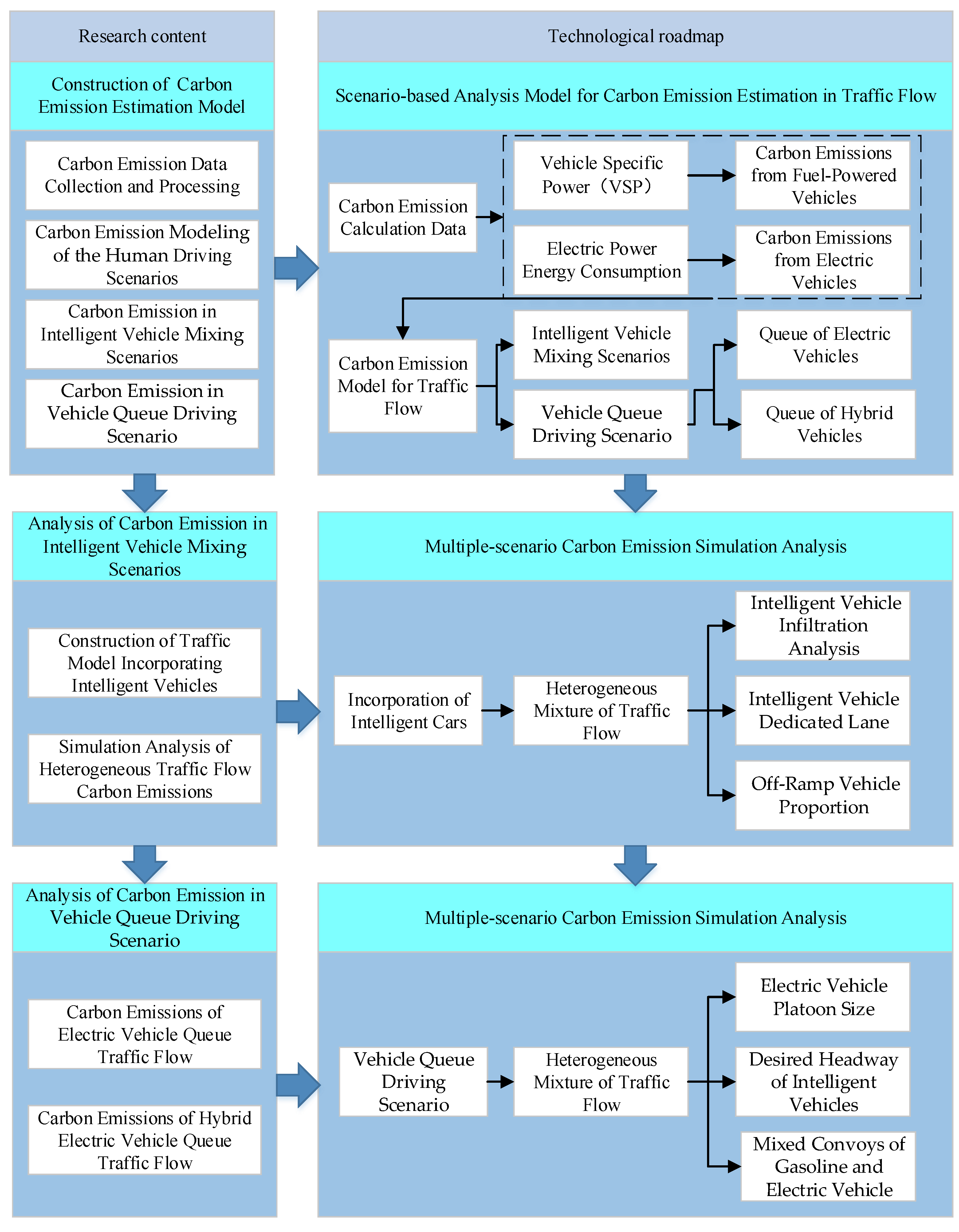
2. Materials and Methods

2.1. Carbon Emission Modeling of the Human Driving Scenarios

Human driving vehicles can be categorized into conventional fuel-powered vehicles and conventional electric vehicles based on their energy consumption characteristics.

2.1.1. Carbon Emission Calculation Model of Fuel Vehicles

Motor vehicle ratio power (VSP) refers to a time unit quality of motor vehicle relating to the corresponding power, which is measured in unit of KW/t or ${\mathrm{m}}^2/{\mathrm{s}}^3$; it requires the engine to overcome wheel rolling resistance (FW), aerodynamic resistance (Fa) and work power due to internal friction (Ff) transmission loss, and it also requires increasing the kinetic energy of the vehicle (Ek) and potential energy (EP) in order to make the power, as shown in Figure 2.

The motor vehicle specific power (VSP) measures the relevant carbon emission index based on the actual work of the motor vehicle, fully considers the driving state of the motor vehicle and the characteristics of the external environment, and can describe the influence of the instantaneous driving behavior of the motor vehicle on the carbon emission. Therefore, this paper uses the VSP method to measure the carbon emission index of traffic flow. According to the relevant literature, the calculation formula of VSP is simplified, and the collated expression is as follows [28]:

$$VSP=\left[1.1a+9.81sin\theta +0.132\right]+0.000302v^3$$

(1)

where a is the instantaneous acceleration of the motor vehicle in $\mathrm{m}/{\mathrm{s}}^2$; $\theta$ is the angle between the road and the horizontal plane, and v is the current instantaneous wind speed in m/s.

According to the above formula, the specific power of a motor vehicle is closely related to its instantaneous speed and acceleration. When the instantaneous speed of the motor vehicle is 0, the VSP is 0; when the motor vehicle accelerates, the VSP is increasing, and the motor vehicle does work; when the motor vehicle slows down, the VSP is decreasing trend, and the motor vehicle power demand is negative; therefore, the specific power of the motor vehicle can reflect the actual driving state of the vehicle as the measurement index of carbon emission of traffic flow.

Then, the emission modeling of fueled cars was completed based on the docking relationship between traffic and the emission of VSP parameters and the emission rate of each pollutant of the vehicle. The principles are as follows.

$$EM={{\displaystyle \sum }}_t^{T}f\left(p_t\right)\times ER\left(p_{t,{\mathrm{co}}_2}\right)$$

(2)

where EM is the total amount of emissions (g) of ${\mathrm{CO}}_2$ from the manually driven fuel vehicle during period t–T, $p_t$ is the value corresponding to VSP at time t, $f\left(p_t\right)$: duration (s) of this VSP interval, the ER ($p_t$, ${\mathrm{CO}}_2$) is the average ${\mathrm{CO}}_2$ emission rate (g/s) of the pt value at time t.

2.1.2. Carbon Emission Calculation Model of Electric Vehicle

The instantaneous power consumption of an electric vehicle is considered as the key parameter and is indirectly converted into carbon dioxide through the power consumed. The instantaneous power consumption model f_e(v, a) of an electric vehicle is a function of the vehicle speed v and acceleration a, which is expressed as follows [29]:

$$f_e\left(v,a\right)\left\{\begin{array}{l}\frac{1}{\eta }\left(\frac{Mg\mu v}{3600}+\frac{C_{d}A{v}^3}{76140}+\frac{\delta Mva}{3600}\right)\hspace{1em}a\ge 0\\ 0 \hspace{1em}\hspace{1em}a<0\end{array}\right.$$

(3)

where $\eta$ is the efficiency of the vehicle transmission system; M is the vehicle mass; g is the gravity acceleration; $\mu$ is the rolling drag coefficient; $C_d$ is the air drag coefficient; A is the vehicle windward area; and $\delta$ is the vehicle rotating mass conversion coefficient.

According to the latest coal consumption of the National Energy Administration of 293.4 g/kw, this follows:

① Reaction form: $\mathrm{O}$ + ${\mathrm{O}}_2$ = ${\mathrm{CO}}_2$;

② Conditions: Standard carbon content 68%; $\mathrm{C}$ molecular weight of 12; ${\mathrm{CO}}_2$ molecular weight of 44; carbon dioxide per per generated of the plant:

$$293.4\times 0.68÷12\times 44=731.5 \left(\mathrm{g}\right)$$

(4)

Carbon emissions of electricity are a major part of the production process, but there are also a series of losses in the transmission and transfer process, as shown in

Table 2. Losses in the process of electricity transmission and transfer.

Loss Source	Ullage
Power grid loss	8%
Loss of power plant itself	The power consumption of 300 MW unit is about 5%, which is calculated as 5%
Charging loss	4%

.

Electric thermal power plants emit carbon dioxide (used in electric vehicles), and 70% of the country’s electricity is generated by thermal power plants. Calculate the available:

$$1\times 70\%÷92\%÷95\%÷96\%\times 731.5=697.5 \left(\mathrm{g}\right)$$

(5)

The carbon emissions generated in time T based on Formulas (3)–(5) are:

$$EC=697.5\times {\sum }_{\Delta T}^T{\sum }_{i=1}^n{f}_e\left(v_i,a_i\right)\times \Delta T$$

(6)

where: EC: carbon dioxide (g) produced by electric vehicle in time T; $f_e \left(v, a\right)$ is the instantaneous power consumption model of the electric vehicle; $i$ is the electric vehicle number.

2.2. Carbon Emission Modeling of the Intelligent Vehicle Mixing Scenario

The intelligent vehicle mixing scenario can be divided into “Traffic Flow Based on Intelligent Vehicles” and “Heterogeneous Traffic Flow”. The distinction between the two lies in the latter’s more detailed scenario description.

2.2.1. Carbon Emission Calculation Model of Traffic Flow Based on Intelligent Vehicles

This section first measures the total carbon emissions from the on-ramp-affected areas.

$$\begin{gathered} E{C}_A={{\displaystyle \sum }}_t^T{{\displaystyle \sum }}_{j=1}^{n_j}{f}_j\left(p_t\right)\times E{R}_j\left(p_{t,c{o}_2}\right)+{{\displaystyle \sum }}_t^T{{\displaystyle \sum }}_{m=1}^{n_m}{f}_m\left(p_t\right)\times E{R}_m\left(p_{t,c{o}_2}\right)+ \\ {\sum }_t^T{\sum }_{i=1}^{n_i}\frac{1}{\eta }\left(\frac{Mg\mu v}{3600}+\frac{C_{d}A{v}^3}{76140}+\frac{\delta Mva}{3600}\right)\times 697.5 \end{gathered}$$

(7)

where $E{C}_A$: for the traffic ${\mathrm{CO}}_2$ emission (g); $p_t$: at time t the value of the corresponding VSP; $f_j\left(p_t\right)$ is the duration (s) of the artificial fuel vehicle j in the VSP interval; $E{R}_j (p_{t,{\mathrm{co}}_2}$) is the VSP of fuel vehicle j at time t is the average emission rate (g/s); $f_e\left(v_i,a_i\right)$: instantaneous emission model of intelligent electric vehicles; $n_j$ for all human-driven fuel vehicles; $n_i$ for all intelligent electric vehicles; $n_m$ for all intelligent fuel vehicles.

2.2.2. Carbon Emission Calculation Model of Heterogeneous Traffic Flow

The specific forms of carbon emission estimation models vary across different scenarios. This section primarily focuses on studying the intelligent vehicle dedicated lane scenario and the scenario based on the proportion of vehicles at off-ramps.

• Carbon emission measurements of intelligent vehicle dedicated lane.

Resistance will change, considering the car and vehicle position as follows:

$$\mathrm{Lead} \mathrm{vehicle}: \mu \left\{\begin{array}{l}-0.7575x^{-1.5225}+1.0325 \hspace{1em} x\le 7.91\\ 1 x>7.91\end{array}\right.$$

(8)

$$\mathrm{Following} \mathrm{vehicle}: \beta \left\{\begin{array}{l}-1.7834x^{-0.0672} \hspace{1em}x\le 55.58\\ 1 x>55.58\end{array}\right.$$

(9)

where $\beta , \mu$ are the air resistance correction coefficients; x is the vehicle spacing in m. When the vehicle is the first car, x is the distance between the vehicle and the rear car; when the vehicle is the follower, x is the distance between the vehicle and the front car.

The contrast movement rate of the vehicle queue and air resistance coefficient in the vehicle’s instantaneous power consumption are modified as shown in (10) and (11).

$$\begin{gathered} VSP=\frac{\frac{d(EK+EP)}{dt}+F_{w}v+F_{a}v+F_{f}v}{m}=v[a(1+\epsilon )+g\times \sin \theta +g\times C_w] \\ +\frac{1}{2m}\times \rho {(v+v_w)}^{2}v\beta (\mu )C_{r}S+C \end{gathered}$$

(10)

$$f_e\left(v,a\right)\left\{\begin{array}{l}\frac{1}{\eta }\left(\frac{Mg\mu v}{3600}+\frac{\beta \left(\mu \right)C_{d}A{v}^3}{76140}+\frac{\delta Mva}{3600}\right) a\ge 0\\ 0 a<0\end{array}\right.$$

(11)

2.

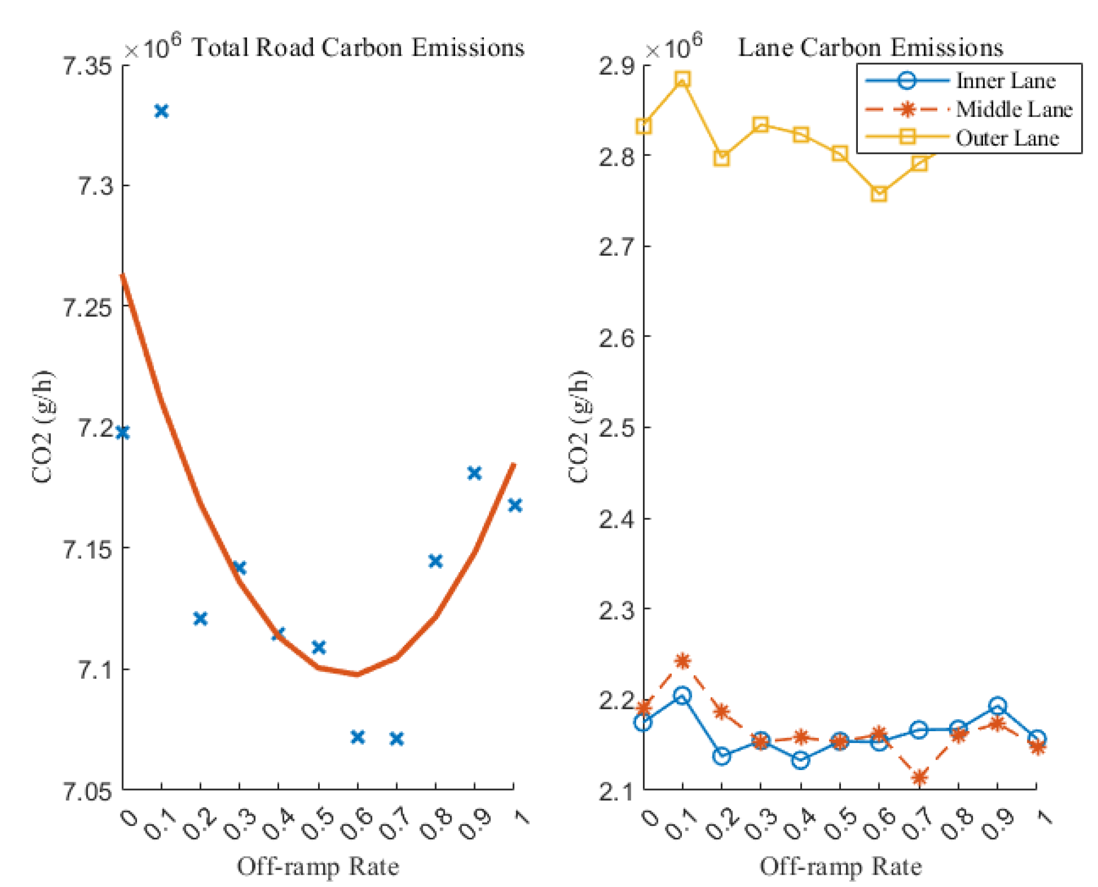
Calculation of carbon emissions based on the proportion of vehicles at off-ramps

The simulation explores the relationship between the exit ramp vehicle occupancy based on 1000 vehicles. The exit ramp occupancy range is set to 0 to 1, and vehicle carbon emissions are measured in hours, as shown in

Table 3. Off-ramp vehicle share and CO₂ emissions in its affected area.

Vehicle Off-Ramp Occupancy	The Carbon Emissions Produced per Hour
0.1	7.20 × 103 g
0.2	7.13 ×103 g
0.3	7.12 × 103 g
0.4	7.11 × 103 g
0.5	7.10 × 103 g
0.6	7.09 × 103 g
0.7	7.12 × 103 g
0.8	7.15 × 103 g
0.9	7.17 × 103 g
1	7.20 × 103 g

. The results obtained by data analysis and fitting show that there is a linear relationship between the off-ramp rate and the carbon emission in the off-ramp influence area, showing the form of quadratic function, which means that with the increase in the off-ramp rate, the carbon emission in the off-ramp influence area will also show a certain change law. This finding provides an important theoretical basis for further research and the optimization of vehicle carbon emissions.

According to existing data, the road carbon emissions calculation formula for the ramp vehicle ratio was obtained, as shown in Formula (12).

$$y=a{x}^2+bx+c$$

(12)

where y is the ${\mathrm{CO}}_2$ emission in the off-ramp affected area affected by the proportion of vehicles at the off-ramp, x is the vehicle proportion at the off-ramp, and a, b, and c are all parameters. After substituting the specific parameters and data, two linear equations, (13) and (14), were obtained.

$$y=0.21x^2-0.505x+7.3\begin{array}{cc}& 0\le x\le 0.7\end{array}$$

(13)

$$y=-8.7x^2+15.8x\begin{array}{cc}& 0.7<x\le 1\end{array}$$

(14)

Based on Equation (12), a carbon emission calculation formula was established for the three lanes of the main expressway affected by the proportion of vehicles on the ramp:

$$\begin{gathered} E{C}_{{}_{L_x}}^d={\displaystyle {\sum }_t^T{\displaystyle \sum _{nu{m}_{nor,L_x}}^{m_{nor}}{f}_{nu{m}_{nor,L_x}}(p_t)\times E{R}_{nor}(p_t,c{o}_2)+{\displaystyle \sum _t^T{\displaystyle \sum _{nu{m}_{dece,}{L}_x}^{m_{dece}}{f}_{nu{m}_{dece,L_x}}}}}}\times E{R}_{dece}(p_t,c{o}_2) \\ +{\displaystyle {\sum }_t^T{\displaystyle \sum _{nu{m}_{acce,L_x}}^{m_{acce}}{f}_{nu{m}_{acce,L_x}}(p_t,{co}_2)\times E{R}_{acce}(p_t,c{o}_2)}} \end{gathered}$$

(15)

where $E{C}_{L_x}^d$ is the carbon emission of the $L_x$ lane affected by the proportion of vehicles on the ramp; $L_x$ is the lane number, the lateral lane, intermediate lane and internal lane are $L_1$, $L_2$, and $L_3$, respectively; $E{R}_{dece}\left(p_{t,{\mathrm{co}}_2}\right)$ is the corresponding emission rate (g/s) during deceleration; $E{R}_{nor}\left(p_{t,{\mathrm{co}}_2}\right)$ is the corresponding emission rate (g/s) during the uniform speed; $E{R}_{acce}\left(p_{t,{\mathrm{co}}_2}\right)$ is the down ramp, $m_{dece}$ is the total number of vehicles; $nu{m}_{nor}$ is the number of vehicles driving on the highway at a uniform speed, a total of $m_{nor}$ vehicles; $nu{m}_{acce}$ is the number of vehicles accelerating on the highway, and $m_{acce}$ is the total number of vehicles (including changing vehicles).

2.3. Carbon Emission Modeling of the Vehicle Queue Driving Scenario

In this subsection, the air resistance correction coefficient and certain parameters of the Cooperative Adaptive Cruise Control (CACC) and Adaptive Cruise Control (ACC) models are considered in the carbon emission model.

2.3.1. Carbon Emissions of Traffic Flow under Electric Vehicle Queue

During the travel of an electric vehicle queue, the carbon emissions of the queue are influenced not only by the queue size but also significantly by the desired headway of intelligent vehicles within the queue.

• Carbon emissions based on the size of the electric fleet

Consider a situation in which the number of electric vehicles mixed in can form a fleet. Assuming that the total number of vehicles in the road section is N; then, all the following vehicles in the fleet will maintain an equilibrium speed when driving. At the same time, the maximum scale of the fleet is n, and the wind resistance correction coefficient is $\beta , \mu$.

$$\begin{gathered} E{C}_d={\displaystyle {\sum }_t^T{\displaystyle \sum _{i=1}^{n_i}{f}_i(p_t)\times E{R}_i(p_t,c{o}_2)+{\displaystyle \sum _t^T{\displaystyle \sum _{j=1}^{n_j}\frac{1}{\eta }(\frac{Mg\mu v_j}{3600}+\frac{\mu C_{d}A{v}_j^3}{76140}+\frac{\delta M{v}_j{a}_j}{3600})}}}}\times 697.5 \\ +{\displaystyle {\sum }_t^T\frac{1}{\eta }\left(\frac{Mg\mu v_e}{3600}+\frac{\beta C_{d}A{v}_e^3}{76140}+\frac{\delta M{v}_e{a}_e}{3600}\right)}\times n_{ci}\times n\times 697.5 \end{gathered}$$

(16)

where $E{C}_d$ is the ${\mathrm{CO}}_2$ emission when the EV queue is not degraded in the heterogeneous traffic flow, $v_e$ is the equilibrium speed when the vehicle travels in a queue, $n_i$ is the human-driven fuel vehicle in the heterogeneous traffic flow, $n_{ci}$ is the number of follower vehicles in queue i, $n_j$ is the first vehicle in all queues, and n is the fleet size.

2.

The carbon emissions based on the expected front time distance of the intelligent vehicle

The following models of ACC and CACC vehicles reflect the relationship of front-time distance in heterogeneous traffic flows and were verified by the PATH laboratory at the University of California, Berkeley.

Suppose that the total number of vehicles in the off-ramp-affected area is sufficiently large, N, where the intelligent vehicle mixing rate is p (p = 1). When p = 1, the degradation of the cruise system is divided into three situations: front of the intelligent vehicle, largest intelligent fleet in front of the intelligent vehicle, and degradation mechanism of the two cruise systems. To facilitate this study, carbon measurement modeling was conducted when the front of the intelligent vehicle reached the largest intelligent fleet.

Assuming that there are i intelligent fleet that have reached the largest n in front, the queue head is artificial following vehicles, the CACC vehicle mixing rate is p (p = 1), the number of CACC vehicles is Np, and the number of ACC vehicles is N∗$\frac{\left(1-p\right)p^{n+1}}{1-p^n}$. Then, the following carbon emission model is:

$$\begin{gathered} E{C}_n^m={\displaystyle {\sum }_t^T{\displaystyle \sum _{k=1}^{n_k}{f}_k(p_t)\times E{R}_k(p_t,c{o}_2)+{\displaystyle \sum _t^T{\displaystyle \sum _{i=1}^{N\ast P}\frac{1}{\eta }(\frac{Mg\mu v_i(t)}{3600}+\frac{\beta C_{d}A{v}_i^3(t)}{76140}+\frac{\delta M{v}_i(t)a_i(t)}{3600})}}}} \\ \times 697.5+{\displaystyle {\sum }_t^T{\displaystyle \sum _{j=1}^{N\ast \frac{(1-p)p^{n+1}}{1-p^n}}\frac{1}{\eta }(\frac{Mg\mu v_j(t)}{3600}+\frac{\beta C_{d}A{v}_j^3(t)}{76140}+\frac{\delta M{v}_j(t)a_j(t)}{3600})}}\times 697.5 \end{gathered}$$

(17)

where $E{C}_n^m$ considers the ${\mathrm{CO}}_2$ emissions generated in the case of CACC degradation caused by the largest intelligent fleet in front of the intelligent vehicle. Here, k is the vehicle queue; i is the vehicle queue CACC follower; j is the vehicle queue ACC follower; the $v_i$(t) is the speed of the CACC vehicle at time t; and $\alpha ,\beta$ is the air resistance correction coefficient of the vehicle leader and the following vehicle respectively.

2.3.2. Carbon Emissions of Traffic Flow under Mixed Queue of Fuel and Electric Fleet

The fuel and electric mixed vehicle queue is introduced, and the carbon emissions are modeled with the proportion of fuel vehicles in the queue and the mixed fleet size as the carbon emission influencing factors affecting the heterogeneous traffic flow.

• The carbon emission calculation is based on the proportion of fuel vehicles in the fleet

Because the carbon emission mode of fuel vehicles is completely different from that of electric vehicles, to further study the carbon emissions of the entire vehicle queue, we explore the proportion of fuel vehicles in the fleet and calculate the carbon emissions of the entire vehicle queue, as shown in Formula (18):

$$\begin{gathered} E{C}_F={\displaystyle {\sum }_t^T{\displaystyle \sum _{p=1}^{n_p}({\displaystyle \sum _{w=1}^{n_w}{f}_w}(p_t)\times E{R}_W(p_t,c{o}_2)+{\displaystyle \sum _{i=1}^{n_i}\frac{1}{\eta }(\frac{Mg\mu v_{ei}}{3600}+\frac{\beta C_{d}A{v}_{ei}^3}{76140}+\frac{\delta M{v}_{ei}{a}_{ei}}{3600})}\times 697.5)}} \\ +{\displaystyle {\sum }_t^T{\displaystyle \sum _{k=1}^{n_k}\frac{1}{\eta }\left(\frac{Mg\mu v_i}{3600}+\frac{\mu C_{d}A{v}_i^3}{76140}+\frac{\delta M{v}_i{a}_i}{3600}\right)\times 697.5}} \end{gathered}$$

(18)

where $E{C}_F$ is the vehicle queue CO₂ emission affected by the proportion of fuel vehicles; $n_p$ has p fleets in the heterogeneous traffic flow; n_i is the number of intelligent electric vehicles following the vehicle queue; n_w is the number of intelligent fuel vehicles following the vehicle queue; $\beta ,\mu$ is the air resistance correction coefficient within the fleet and the head vehicle, respectively; $v_{ei}$ is the equilibrium speed of the following vehicles in fleet i.

After the carbon emission measurement of the vehicle queue is affected by the proportion of fuel vehicles in the fleet, the carbon emission modeling of the fuel-electric mixed heterogeneous traffic flow continues, as shown in (19).

$$\begin{gathered} E{C}_F^q={\displaystyle {\sum }_t^T{\displaystyle \sum _{p=1}^{n_p}\left({\displaystyle \sum _{w=1}^{n_w}{f}_w\left(p_t\right)\times E{R}_{\mathrm{w}}\left(p_t,c{o}_2\right)}+{\displaystyle \sum _{i=1}^{n_i}\frac{1}{\eta }\left(\frac{Mg\mu v_{\mathrm{ei}}}{3600}+\frac{\mu C_{\mathrm{d}}A{v}_{ei}^3}{76140}+\frac{\delta M{v}_{ei}{\alpha }_{ei}}{3600}\right)\times 697.5}\right)}} \\ +{\displaystyle {\sum }_t^T\left[{\displaystyle \sum _{k=1}^{n_k}\frac{1}{\eta }\left(\frac{Mg\mu v_i}{3600}+\frac{\mu C_{d}A{v}_i^3}{76140}+\frac{\delta M{v}_i{a}_i}{3600}\right)\times 697.5+{\displaystyle \sum _{j=1}^{n_i}{f}_j\left(p_j\right)\times E{R}_j\left(p_t,c{o}_2\right)}}\right]} \end{gathered}$$

(19)

where: $E{C}_F^q$ is the carbon emission of heterogeneous traffic flow affected by the proportion of fuel vehicles in the mixed fleet, $n_j$ is the manually driven fuel vehicle; and the other parameters are listed above.

2.

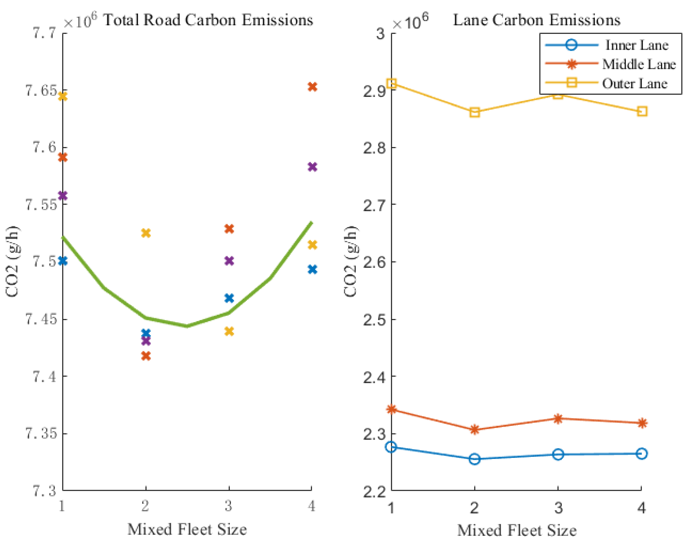
Carbon emission measurement based on mixed fleet size

This section assumes that the intelligent-vehicle queue is a fuel and electric mixed queue, the first queue is an electric vehicle, and the number of vehicles in the queue is equal (n vehicles). To explore carbon emission measurements of heterogeneous traffic flows in an off-ramp impact area, see the equations in (20),

$$\begin{gathered} E{C}_{ef}={\displaystyle {\sum }_t^T\left[{\displaystyle \sum _{w=1}^{n_w}{f}_w\left(p_t\right)\times E{R}_w\left(p_t,c{o}_2\right)}+{\displaystyle \sum _{i=1}^{n_i}\frac{1}{\eta }\left(\frac{Mg\mu v_{\mathrm{i}}}{3600}+\frac{\beta C_{d}A{v}_i^3}{76140}+\frac{\delta M{v}_i{\alpha }_i}{3600}\right)\times 697.5}\right]}\times \left(n-1\right) \\ {\displaystyle {\sum }_t^T\left[{\displaystyle \sum _{\mathrm{j}=1}^{n_j}\frac{1}{\eta }\left(\frac{Mg\mu v_{\mathrm{ei}}}{3600}+\frac{\mu C_{d}A{v}_{\mathrm{ei}}^3}{76140}+\frac{\delta M{v}_{\mathrm{ei}}{\alpha }_{\mathrm{ei}}}{3600}\right)\times 697.5+{\displaystyle \sum _{k=1}^{n_k}{f}_k\left(p_t\right)\times E{R}_k\left(p_t,c{o}_2\right)}}\right]} \end{gathered}$$

(20)

where $E{C}_{ef}$ is the emission of heterogeneous traffic flow ${\mathrm{CO}}_2$ considering the mixed fleet size, $n_w$ is the number of intelligently connected fuel-following vehicles in the mixed fleet, $n_i$ is the number of intelligently connected electric-following vehicles in the mixed fleet, n is the number of intelligently connected fleet vehicles, $n_j$ is the number of head vehicles in the off-ramp influence zone within time t, and $n_k$ is all human-driven vehicles.

2.4. Data Collection and Traffic Flow Modeling Parameter Calibration

2.4.1. Traffic and Carbon Emissions Data Collection

The survey site of traffic flow and vehicle composition data was selected from the off-ramp sections of Weiyang Interchange, LvXiaozhai Interchange and Zhangba Interchange of the Xi’an City Bypass Expressway, and the survey time was from 26 March 2022 to 3 April 2022. An RTMS was used to collect data on road traffic flow, and each survey site was investigated for a total of 75 min.

This study utilizes an onboard exhaust gas detection equipment Portable Emission Measurement System (PEMS) to estimate motor vehicle exhaust emissions. Carbon emissions data collection took place in the section from the Lvxiaozhai Interchange to the Zhangba Interchange

2.4.2. Parameter Calibration

• Car-Following Models

• Manual Car-Following Model

The intelligent driver model (IDM) was selected as the car-following model for manually driven vehicles [19]. A genetic algorithm was employed to optimize the parameters. The population size and the maximum number of iterations were set to 500. The calibration results of the car-following model are as follows (

Table 4. Calibration Results of the IDM Model.

Parameter	${\mathit{v}}_{\mathit{m}\mathit{a}\mathit{x}}\left(\mathbf{m}/\mathbf{s}\right)$	${\mathit{a}}_{\mathit{m}}\left(\mathbf{m}/{\mathbf{s}}^2\right)$	${\mathit{b}}_{\mathit{n}}\left(\mathbf{m}/{\mathbf{s}}^2\right)$	${\mathit{T}}_{\mathit{s}}\left(\mathbf{s}\right)$	${\mathit{s}}_0\left(\mathbf{m}\right)$
value	30	2.3	3.6	2.0	1.5

).

• Autonomous Car-Following Model

Path laboratory team carried out research on car following model of autonmous vehicle traffic flow earlier, and the proposed model is widely used in the research on traffic flow characteristics of autonomous vehicle [30]. The acceleration of ACC vehicles is determined by the gap error and the difference in velocity with respect to the preceding vehicle. The ACC model is as follows [30,31]:

$$e_s(t)=\Delta x(t)-t_a{v}_s(t)-l-s_0$$

(21)

$$a_s(t)=k_1{e}_s(t)+k_2\Delta v$$

(22)

where $e_s\left(t\right)$ is the difference between the ACC vehicle’s workshop distance at the first moment and the desired workshop distance; $\mathsf{\Delta }x\left(t\right)$ is the headway between the following vehicle and the leading vehicle at the moment t; $t_a$ is the desired workshop time distance set by the driver; $l$ is the body length; $s_0$ is the workshop distance at the time of congestion; $a_s\left(t\right)$ is the acceleration of the ACC vehicle at the moment t; $\mathsf{\Delta }v$ is the speed difference between the following vehicle and the leading vehicle; $k_1$ and $k_2$ are the adjustment coefficient. See

Table 5. Parameter Values for the ACC Car-Following Model.

Parameters	$\mathit{l}$	${\mathit{s}}_0$	${\mathit{k}}_1$	${\mathit{k}}_2$	${\mathit{t}}_{\mathit{M}\mathit{V}}$
Value	5	2	0.23	0.07	1.6

and

Table 6. Constant Time Gaps for ACC Vehicles.

$\mathbf{Constant} \mathbf{Time} \mathbf{Gap} {\mathit{t}}_{\mathit{a}}$ (s)	1.1	1.6	2.2
Proportion (%)	50.4	18.5	31.1

.

The CACC model expression is as follows [29]:

$$e_s(t-1)=\Delta x(t-1)-t_c{v}_s(t-1)-l-s_0$$

(23)

$$v_s(t)=v_s(t-1)+k_p{e}_s(t-1)+k_d{e}_s^{\prime }(t-1)$$

(24)

where $e_s\left(t-1\right)$ represents the gap error of the CACC vehicle at time $t-1$; $\Delta x\left(t-1\right)$ represents the headway between the following vehicle and the leading vehicle at time $t-1$; $t_c$ is the pre-set desired time headway; $l$ is the vehicle length; $s_0$ is the distance between vehicles in congested conditions; $v_s\left(t\right)$ is the velocity of the CACC vehicle at time t; $v_s\left(t-1\right)$ is the velocity of the CACC vehicle at the previous time $t-1$; $e_s^{\prime }\left(t-1\right)$ represents the derivative of the gap error at time $t-1$, i.e., the increment of the gap error per unit time; $k_p$ and $k_d$ are adjustment coefficients. See

Table 7. Parameter Values for the CACC Car-Following Model.

Parameters	$\mathit{l}$	${\mathit{s}}_0$	${\mathit{k}}_{\mathit{p}}$	${\mathit{k}}_{\mathit{d}}$	${\mathit{t}}_{\mathit{M}\mathit{V}}$
value	5	2	0.45	0.25	1.6

and

Table 8. Constant Time Gaps for CACC Vehicles.

$\mathbf{Constant} \mathbf{Time} \mathbf{Gap} {\mathit{t}}_{\mathit{c}}$ (s)	0.6	0.7	0.9	1.1
Proportion (%)	57.0	24.0	7.0	12.0

.

2.

Lane Change Model

During each lane change, vehicles must assess the presence of a lane-changing motive and allowable gap for lane changing. The probability of a vehicle changing lanes, denoted as $P_{change lanes}$, consists of two components: the lane-changing motive generation probability $P_{motivation}$, and the lane-changing gap acceptance probability $P_{acceptance}$.

$$P_{change lane}=P_{motivation}\times P_{acceptance}$$

(25)

The calculations of $P_{motivation}$ and $P_{acceptance}$ are based on the model proposed by Liu [32]. The maximum likelihood estimation method was used to calibrate the motivation generation model parameters using 100 lane change events extracted from GPS aerial videos. The calibration results are presented in

Table 9. Coefficients of Lane Change Model Calibration.

Parameter	${\mathit{E}}_{\mathit{m}\mathit{a}\mathit{x}}$	${\mathit{E}}_{\mathit{m}\mathit{i}\mathit{n}}$	${\mathit{a}}_1$	${\mathit{a}}_2$
Value	260 m	160 m	0.036	0.016

.

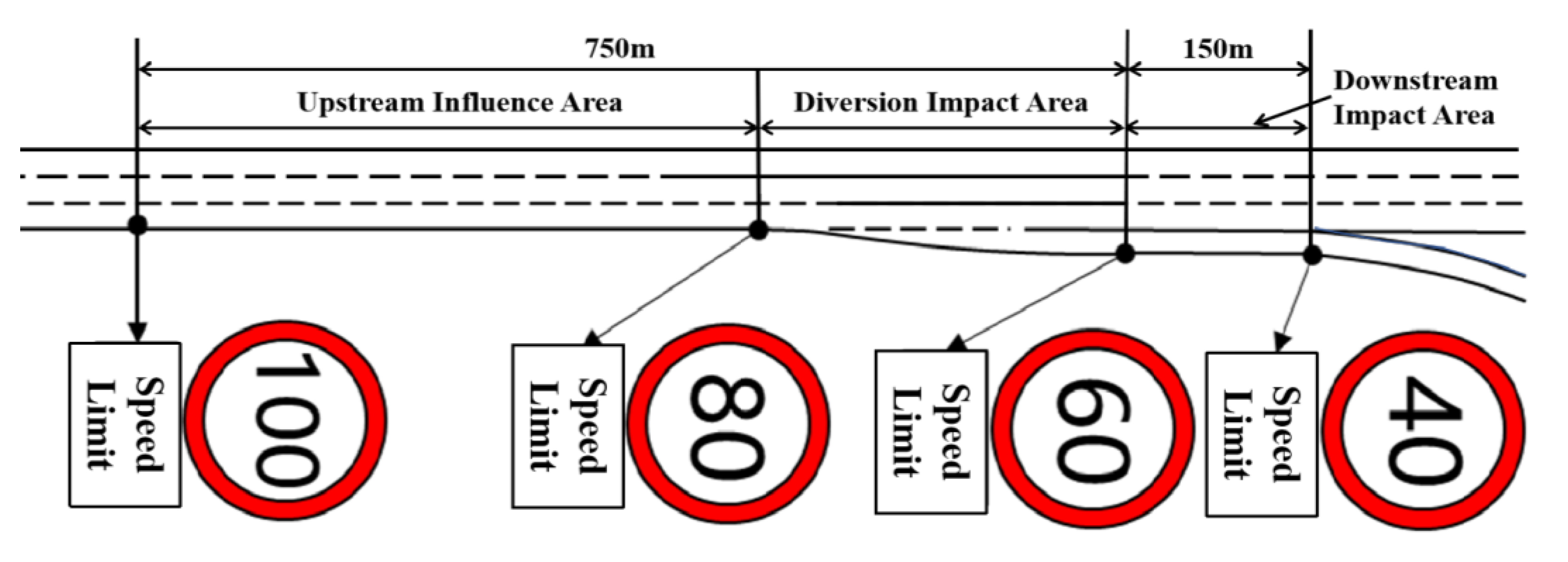
2.5. Simulation Experiment Scenarios

2.5.1. Simulation Scenario

To investigate the impacts of various factors on carbon emissions in heterogeneous traffic flows, a three-lane simulation scenario was constructed based on the actual situation in the downstream diversion section of the Xi’an Ring Expressway, as shown in Figure 3.

The entire road segment consisted of a mainline, a deceleration lane, and an off-ramp. The mainline consists of three lanes: an inner, middle, and outer. The deceleration lanes were parallel to each other. Speed control was implemented through a cascaded speed limit scheme with the vehicle speed limits set successively at 100, 80, and 60 km/h. The speed limit for the vehicles on the off-ramp was 40 km/h. The lane separators were marked using graded markings. Within 200 m upstream of the diversion point, lane changes from the inner lane to the middle lane were prohibited, and lane changes from the middle lane to the outer lane were prohibited after the diversion point.

2.5.2. Simulation Design

MATLAB was used to conduct simulation experiments under the aforementioned simulation scenarios and conditions to explore the characteristics of the heterogeneous traffic flow. The simulation designs for the various scenarios are as follows (

Table 10. Summary of Simulation Designs.

Experimental Category		Vehicle Type	Parameter Values
Influence Factor Analysis	Intelligent Vehicle Infiltration Rate	Manual Vehicle (Fuel) Intelligent Vehicle (Fuel)	P = 0, 10%, 20%, 30%, 40%, 50%, 60%, 70%, 80%, 90%, 100%
	Percentage of Vehicles Exiting the Ramp		P = 40%; ${\mathrm{P}}_{\mathrm{off}}$ = 0%, 10%, 20%, 30%, 40%, 50%, 60%, 70%, 80%, 90%, 100%
	Dedicated Lane for Autonomous Vehicles		P = 0, 10%, 20%, 30%, 40%, 50%, 60%, 70%, 80%, 90%, 100%
Analysis of Carbon Emissions in Electric Vehicle Fleets	Scale of Electric Vehicle Fleet	Manual Vehicle (Fuel) Intelligent Vehicle (Fuel)	P = 40%; N = 1, 2, 3, 4
	Desired Time Headway of Intelligent Vehicles	Manual Vehicle (Fuel) Intelligent Vehicle (Electric)	tc = 0.6 s; ta = 1.1, 1.6, 2.2 s; P = 0, 10%, 20%, 30%, 40%, 50%, 60%, 70%, 80%, 90%, 100%
			ta = 1.1 s; tc = 0.6, 0.9, 1.1 s; P = 0, 10%, 20%, 30%, 40%, 50%, 60%, 70%, 80%, 90%, 100%
	Mixed Fleet Size		P = 40%; N = 1, 2, 3, 4

).

3. Results

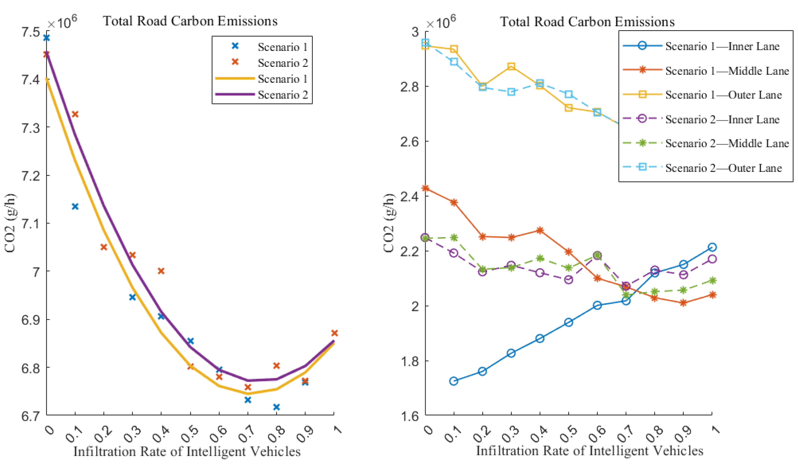
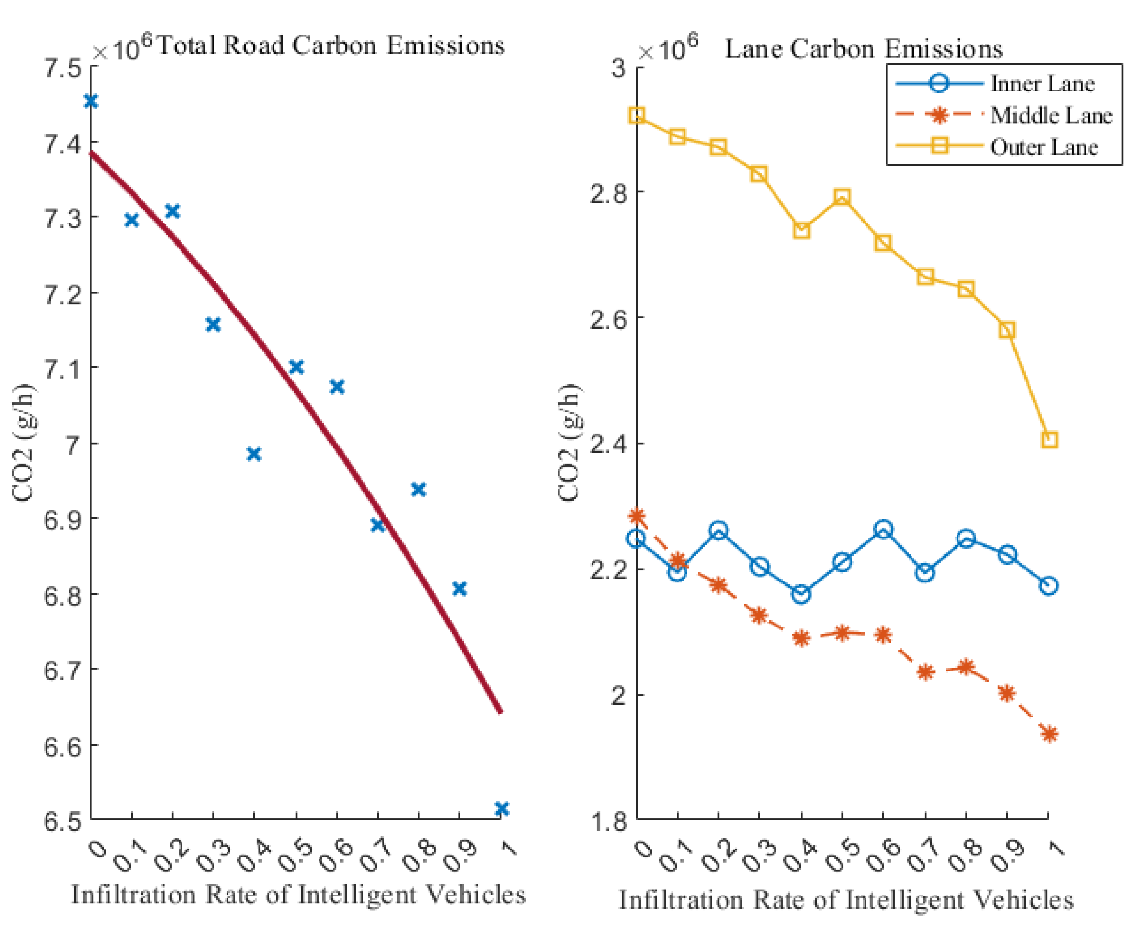
3.1. Intelligent Vehicle Infiltration Scenario Experiment

3.1.1. Intelligent Vehicle Infiltration Analysis

The trends in the overall carbon emissions of the road and the carbon emissions of each lane under different intelligent vehicle infiltration rates obtained in the previous traffic scenarios are shown below.

In Figure 4, the results indicate that the total road carbon emissions decreased as the infiltration rate of intelligent vehicles increased, with a higher rate of decrease. The carbon emissions for each lane show a similar trend, with the outer lane experiencing a significant decrease and a faster rate of decrease. The carbon emissions for the inner lane fluctuated but remained relatively stable, whereas those for the middle lane exhibited a consistent and stable decrease. The markings in the figure are intended to represent the results of different experiments, with each point being the average of ten experiments. The same applies to the following text.

Intelligent vehicles, equipped with ACC/CACC systems for information acquisition and response to external stimuli, exhibit reduced reaction times and improved desired gaps. With the increasing presence of intelligent vehicles, the average admissible gap among vehicles on the road diminishes, resulting in enhanced road operations and a consequent reduction in carbon emissions associated with the rise in the penetration rate of intelligent vehicles. For vehicles requiring off-ramp exits, swift lane merging into the outer lane is achievable, contributing to congestion mitigation. Consequently, carbon emissions in both the outer and middle lanes exhibit a declining trend. However, the outer lane’s capacity to accommodate vehicles bound for off-ramps is limited. When the middle lane accumulates a significant number of vehicles exiting, those choosing to continue on the main road opt for the more advantageous inner lane, thus experiencing a heightened inflow of mainline vehicles, leading to fluctuations in carbon emissions within the inner lane.

3.1.2. Intelligent Vehicle Dedicated Lane

The effectiveness of setting dedicated lanes for intelligent vehicles under the conditions of smart-car infiltration remains unclear. This section will focus on setting the inner lane of a three-lane highway as a dedicated lane for intelligent vehicles. Scenario 1 represents the presence of a dedicated lane for intelligent vehicles, and Scenario 2 represents the absence of a dedicated lane for intelligent vehicles.

Figure 5 shows the total carbon emissions on the road and the carbon emissions in each lane with and without the implementation of a single dedicated lane for intelligent vehicles. Setting a single dedicated lane for intelligent vehicles can reduce carbon emissions on the road, and the reduction effect initially increases and then decreases with an increasing intelligent vehicle infiltration rate. Carbon emissions in the middle and outer lanes decreased as the intelligent vehicle infiltration rate increased, whereas carbon emissions in the inner lane increased as the intelligent vehicle infiltration rate increased. As the implementation of a dedicated lane for intelligent vehicles on the inner side of the road occurs, with the rising proportion of intelligent vehicles, they gravitate toward traveling in this exclusive lane. Consequently, there is a surge in traffic flow and a heightened occurrence of congestion within the dedicated lane for intelligent vehicles, ultimately resulting in a proportional escalation of carbon emissions. By comparing the carbon emissions with and without a dedicated inner lane for intelligent vehicles, it is evident that the middle lane is significantly affected and gradually transfers to the inner lane with an increase in the infiltration rate.

3.1.3. Off-Ramp Vehicle Proportion

In the highway diversion area section, the vehicle off-ramp is an important driving behavior, controlling 40% of intelligent vehicles and 60% of manually driven vehicles to obtain the following carbon emission graph:

In Figure 6, with the increase in off-ramp rate, the total carbon emission of the road tends to decrease and then increase, and it reaches the lowest value at 60% of the off-ramp rate; in addition, at each off-ramp rate, the carbon emission value of the inner lane and the middle lane is lower, the carbon emission value of the outer lane is the highest, and the carbon emission curve of each lane also tends to decrease and then increase with the increase in off-ramp rate. As the off-ramp rate increases, the outer lane has the highest carbon emission value because it must carry all off-ramp vehicles. When the off-ramp rate is low, the vehicles can pass through the diversion area without congestion, and the carbon emission value decreases. When the off-ramp rate is high, the number of vehicles on the off-ramp is larger than the capacity of the off-ramp provided by the road, resulting in congestion, which causes the carbon emission value to increase.

As off-ramp rates increase, the outer lane experiences a surge in carbon emissions due to the accumulation of departing vehicles. The outer lane bears the responsibility of accommodating all vehicles exiting the road. However, due to the limited space available in the deceleration lanes, a threshold is established that governs the maximum number of vehicles that can navigate the off-ramp area within a given timeframe. When the off-ramp rate remains at a moderate level, vehicles can smoothly maneuver through the diversion area, avoiding congestion and subsequently reducing carbon emissions. Conversely, during periods of high off-ramp rates, an overflow of vehicles exceeding the road’s capacity upon exiting leads to congestion, resulting in an increase in carbon emissions.

3.2. Intelligent Vehicle Platoons Scenario Experiment

3.2.1. Electric Vehicle Platoon Size

A hybrid flow of gasoline and electric vehicles, owing to their different energy consumption methods and the adoption of smart driving modes, can have new impacts on road traffic and carbon emission characteristics. When electric vehicles accounted for 40% of the hybrid flow and gasoline vehicles accounted for 60%, the simulation results showing the impact of different electric vehicle fleet sizes on road carbon emissions are depicted in Figure 7.

In Figure 7, it can be observed that in a mixed flow of conventional fuel vehicles and electric vehicles, when electric vehicles are organized in platoons, road carbon emissions exhibit a decreasing trend with an increase in platoon size. Carbon emissions reached a minimum value at N = 2. Among the different platoon sizes, the outer lane had the highest carbon emissions, followed by the inner lane, whereas the middle lane had the lowest carbon emissions. Carbon emissions showed similar trends in all lanes; however, the inner lane exhibited greater variation.

The implementation of CACC (Cooperative Adaptive Cruise Control) systems empowers electric vehicle platoons to establish intelligent interconnected vehicle convoys, facilitating efficient and seamless information exchange among convoy vehicles. When the intelligent vehicle convoy is relatively short, enhanced inter-vehicle communication through V2V (Vehicle-to-Vehicle) communication enhances traffic flow stability on the road. However, when the convoy length surpasses a certain threshold, a succession of intelligent vehicle convoys converges into a dynamic “bottleneck”, impeding traffic flow and resulting in increased congestion and disarray, ultimately leading to a rise in carbon emissions.

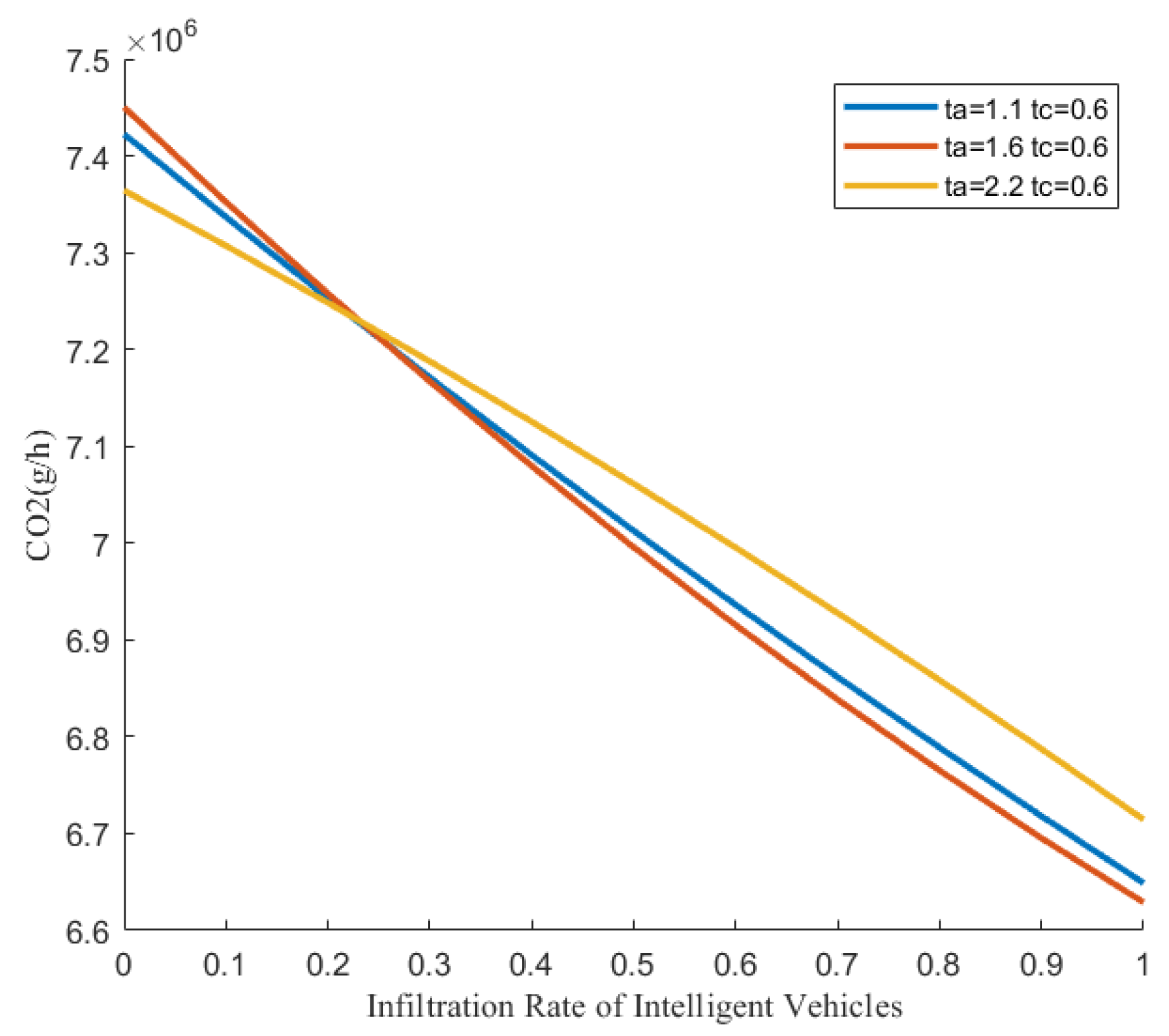
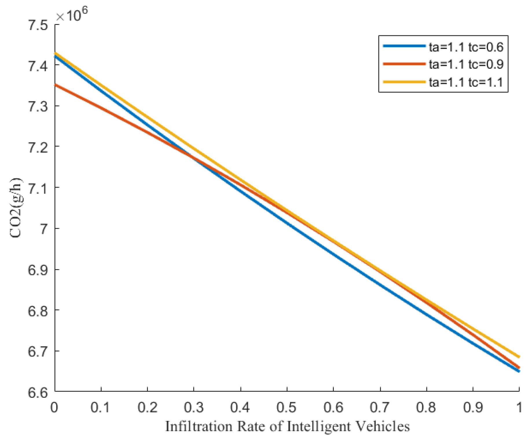
3.2.2. Desired Headway of Intelligent Vehicles

The key factor in the operation of intelligent vehicles is the desired headway between vehicles. Under the condition of a platoon size N set to 2, the desired headways of both the ACC and CACC vehicles were varied to investigate their impact on carbon emissions.

• Impact of desired headway of ACC vehicles on traffic flow carbon emissions.

Maintaining the desired headway of the CACC vehicles ($t_c$) at 0.6, the desired headway of the ACC vehicles was set to 1.1 s, 1.6 s, and 2.2 s, respectively. The simulation results show the carbon emission variation curves for each condition in Figure 8.

In Figure 8, it can be observed that under all conditions, road carbon emissions decreased as the infiltration rate (P) of intelligent vehicles increased, which is consistent with previous research findings. Additionally, as the desired headway of the ACC vehicles increased, the downward trend of the carbon emissions curve became less steep. The curves can be divided by P = 24%, where for p values lower than this threshold, the road carbon emissions reach a low value at a larger ACC desired headway of 2.2 s. Conversely, for p values greater than the threshold, the emissions reach a low value at a smaller desired headway of 1.6 s. This indicates that the optimal desired headway for achieving low carbon emissions varies with different infiltration rates of intelligent vehicles, and a specific analysis based on the specific situation is required.

The adjustment of the “Ta” parameter is anticipated to wield a considerable influence on the ensuing behavioral paradigms displayed by intelligent vehicles. When confronted with scenarios marked by a sparser distribution of intelligent vehicles, the rationale for maintaining a more substantial interval between these pioneering vehicles and their conventional counterparts becomes readily apparent. Such a strategy confers the latter with an extended response window, efficaciously tempering assertive driving behaviors, including abrupt accelerations or decelerations. Conversely, within contexts characterized by a denser presence of intelligent vehicles, the inter-vehicle communication facilitated through onboard systems endows meticulous control over diminished trailing distances. This strategic arrangement augments the seamless and expedited flow of traffic, thereby culminating in a palpable reduction in carbon emissions along the thoroughfare.

2.

Impact of desired headway of CACC vehicles on traffic flow carbon emissions.

Compared to the desired headway at 1.1 s, the desired headway of CACC vehicles was varied as 0.6 s, 0.9 s, and 1.1 s, respectively. The carbon emission variation curves for each condition are shown in Figure 9.

In Figure 9, it can be observed that the carbon emissions curves under different conditions are more closely packed together. This indicates that the desired headway for CACC vehicles has a limited overall impact on the road carbon emissions. However, at tc = 1.1 s, the overall carbon emissions are generally higher. For p values below 30%, the desired headway ($t_c$ = 0.9 s) results in lower carbon emissions, whereas for p values above 30%, the desired headway (($t_c$ = 0.6 s) leads to lower carbon emissions. Therefore, it can be concluded that the optimal desired headway of CACC vehicles for achieving low carbon emissions varies with the different infiltration rates of intelligent vehicles, and changing ($t_c$ does not have a significant effect.

The adjustment of the “t_c” parameter has a significant impact on the behavior of intelligent vehicle formations. When there are few intelligent vehicles on the road, a small gap between vehicles can lead to more aggressive driving behaviors among conventional vehicles. On the other hand, a large following distance can cause intelligent vehicle formations to become bottlenecks on the road, disrupting the flow of nearby vehicles. As a result, both scenarios contribute to increased carbon emissions.

Conversely, as the number of intelligent vehicles on the road increases, there is a higher likelihood of forming intelligent vehicle formations. Adhering to a shorter following distance enhances traffic efficiency, which in turn reduces carbon emissions along this traffic route.

3.2.3. Mixed Convoys of Gasoline and Electric Vehicle

In the current scenario of mixed gasoline and electric traffic flows adopting a convoy driving strategy, with electric vehicles accounting for 40% and gasoline vehicles accounting for 60% of the total, the impact of convoy size on carbon emissions from traffic flow is shown in the following graph:

As shown in Figure 10, when both gasoline and electric vehicles adopt the convoy driving strategy, the total road carbon emissions decrease, which is followed by an increase as the maximum convoy length increases. Minimum carbon dioxide emissions were achieved when N was approximately 2–3, and the specific value varied with the desired headway times of the vehicles. Furthermore, the outer lane has the highest road carbon emissions, whereas the middle lane has the lowest. The carbon emissions trend of the three lanes aligns with the overall trend of the total carbon emissions.

A combination of fuel vehicles and electric vehicles constitutes a blended fleet, which is guided by the CACC system for their following and lane-changing actions. Consequently, the patterns demonstrated by the mixed fleet in relation to convoy size align closely with those observed in electric vehicle convoys. Since fuel vehicles are integrated into the convoy composition, the collective carbon emissions of the fleet are lower compared to a convoy exclusively comprising electric vehicles.

4. Discussion and Conclusions

Based on the scenario analysis, three typical traffic flow scenarios were proposed: manual driving scenario, intelligent vehicle mixing scenario, and vehicle convoy scenario, considering the future conditions of vehicle networking, intelligence, and mixed traffic with different levels of driving automation. Data collection was conducted and microscopic traffic flow models were calibrated for three interchanges on the Xi’an Ring Expressway. Through simulation experiments, the carbon emission characteristics of traffic flow under each scenario were revealed. The results indicated that carbon emissions decreased with an increase in the intelligent vehicle mixing rate. The implementation of a dedicated lane for intelligent vehicles helps reduce carbon emissions. Carbon emissions showed an initial decreasing trend and then increased with an increase in vehicles exiting the off-ramp. Adjusting the headway between ACC and CACC vehicles can reduce carbon emissions under different intelligent vehicle mixing rates. In the case of vehicle convoy driving, both electric vehicle convoys and mixed convoys of gasoline and electric vehicles had minimum carbon emissions when they were composed of two vehicles. This research provides methodological support for exploring the carbon emission characteristics of heterogeneous traffic flow in off-ramp impact areas after the widespread adoption of intelligent vehicles and serves as a basis for formulating low-carbon development strategies for future highway systems.

References

1. Zhang, L.; Long, R.; Chen, H.; Geng, J. A review of China’s road traffic carbon emissions. J. Clean. Prod. 2019, 207, 569–581. [Google Scholar] [CrossRef]
2. Talebpour, A.; Mahmassani, H.S. Influence of connected and autonomous vehicles on traffic flow stability and throughput. Transp. Res. Part C Emerg. Technol. 2016, 71, 143–163. [Google Scholar] [CrossRef]
3. Rios-Torres, J.; Malikopoulos, A.A. A survey on the coordination of connected and automated vehicles at intersections and merging at highway on-ramps. IEEE Trans. Intell. Transp. Syst. 2017, 18, 1066–1077. [Google Scholar] [CrossRef]
4. Yao, Z.; Wang, Y.; Liu, B.; Zhao, B.; Jiang, Y. Fuel consumption and transportation emissions evaluation of mixed traffic flow with connected automated vehicles and human-driven vehicles on expressway. Energy 2021, 230, 120766. [Google Scholar] [CrossRef]
5. Xiao, L.; Gao, F. Practical string stability of platoon of adaptive cruise control vehicles. IEEE Trans. Intell. Transp. Syst. 2011, 12, 1184–1194. [Google Scholar] [CrossRef]
6. Zheng, S.; Li, H.; Huang, Z.; Li, K.; Qin, L. Flow-balanced-based collaborative strategies and simulation of vehicle group behaviors for on-ramp areas. Simul. Model. Pract. Theory 2020, 103, 102093. [Google Scholar] [CrossRef]
7. Golob, T.F.; Recker, W.W.; Alvarez, V.M. Safety aspects of freeway weaving sections. Transp. Res. Part A Policy Pract. 2004, 38, 35–51. [Google Scholar] [CrossRef]
8. Zheng, Y.; Ran, B.; Qu, X.; Zhang, J.; Lin, Y. Cooperative lane changing strategies to improve traffic operation and safety nearby freeway off-ramps in a connected and automated vehicles environment. IEEE Trans. Intell. Transp. Syst. 2020, 21, 4605–4614. [Google Scholar] [CrossRef]
9. Yang, K. The Effects of Safety Deceleration Rule in Traffic System. Appl. Mech. Mater. 2014, 496, 3013–3016. [Google Scholar] [CrossRef]
10. Hancock, M.W.; Wright, B. A Policy on Geometric Design of Highways and Streets; American Association of State Highway and Transportation Officials: Washington, DC, USA, 2013. [Google Scholar]
11. Gong, J.; Guo, X.; Dai, S.; Duan, L. Research on the Operational Characteristics of Diverging Area on Expressway Off-ramp based on Different Restricted Strategy of Lane. Procedia Soc. Behav. Sci. 2013, 96, 1156–1164. [Google Scholar] [CrossRef]
12. Davis, L.C. Effect of adaptive cruise control systems on traffic flow. Phys. Rev. E 2004, 69, 066110. [Google Scholar] [CrossRef] [PubMed]
13. Schleicher, S.; Gelau, C. The influence of Cruise Control and Adaptive Cruise Control on driving behaviour—A driving simulator study. Accid. Anal. Prev. 2011, 43, 1134–1139. [Google Scholar] [CrossRef]
14. Davis, L.C. Stability of adaptive cruise control systems taking account of vehicle response time and delay. Phys. Lett. A 2012, 376, 2658–2662. [Google Scholar] [CrossRef]
15. Siebert, F.W.; Oehl, M.; Pfister, H.R. The influence of time headway on subjective driver states in adaptive cruise control. Transp. Res. Part F Traffic Psychol. Behav. 2014, 25, 65–73. [Google Scholar] [CrossRef]
16. Milanés, V.; Shladover, S.E.; Spring, J.; Nowakowski, C.; Kawazoe, H.; Nakamura, M. Cooperative adaptive cruise control in real traffic situations. IEEE Trans. Intell. Transp. Syst. 2013, 15, 296–305. [Google Scholar] [CrossRef]
17. Rupp, A.; Stolz, M.; Horn, M. Decentralized cooperative merging using sliding mode control. IFAC Pap. Online 2018, 51, 349–354. [Google Scholar] [CrossRef]
18. Treiber, M.; Hennecke, A.; Helbing, D. Congested traffic states in empirical observations and microscopic simulations. Phys. Rev. E 2000, 62, 1805. [Google Scholar] [CrossRef]
19. Alam, A.; Hatzopoulou, M. Modeling transit bus emissions using MOVES: Comparison of default distributions and embedded drive cycles with local data. Transp. Eng. Part A Syst. 2017, 143, 04017049. [Google Scholar] [CrossRef]
20. Farzaneh, M.; Zietsman, J.; Lee, D.-W.; Johnson, J.; Wood, N.; Ramani, T.; Gu, C. Texas-Specific Drive Cycles and Idle Emissions Rates for Using with EPA’s MOVES Model-Final Report; Texas Department of Transportation: Austin, TX, USA, 2014.
21. Yuxi, Z.; Zongtao, D.; Yishui, Z.H.U.; Wang, L.; Zhou, Y.; Guo, Y. Survey of Fuel Consumption Model for Motor Vehicle. J. Comput. Eng. Appl. 2021, 57, 14–26. [Google Scholar]
22. Chaudhari, A.R.; Thring, R.H. Energy economy analysis of the G-Wiz: A two-year case study based on two vehicles. Proc. Inst. Mech. Eng. Part D J. Automob. Eng. 2011, 225, 1505–1517. [Google Scholar] [CrossRef]
23. Zhang, R.; Yao, E. Electric vehicles’ energy consumption estimation with real driving condition data. Transp. Res. Part D 2015, 41, 177–187. [Google Scholar] [CrossRef]
24. Genikomsakis, K.N.; Mitrentsis, G. A computationally efficient simulation model for estimating energy consumption of electric vehicles in the context of route planning applications. Transp. Res. Part D 2017, 50, 98–118. [Google Scholar] [CrossRef]
25. Wu, X.; Freese, D.; Cabrera, A.; Kitch, W.A. Electric vehicles’ energy consumption measurement and estimation. Transp. Res. Part D 2015, 34, 52–67. [Google Scholar] [CrossRef]
26. Yang, H.; Rakha, H.; Ala, M.V. Eco-cooperative adaptive cruise control at signalized intersections considering queue effects. IEEE Trans. Intell. Transp. Syst. 2016, 18, 1575–1585. [Google Scholar] [CrossRef]
27. Wang, Z.; Wu, G.; Hao, P.; Boriboonsomsin, K.; Barth, M. Developing a platoon-wide eco-cooperative adaptive cruise control (CACC) system. In Proceedings of the 2017 IEEE Intelligent Vehicles Symposium (IV), Los Angeles, CA, USA, 11–14 June 2017; pp. 1256–1261. [Google Scholar] [CrossRef]
28. Yao, E.; Wang, M.; Song, Y.; Zhang, Y. Estimating Energy Consumption on the Basis of Microscopic Driving Parameters for Electric Vehicles. Transp. Res. Rec. J. Transp. Res. Board 2014, 2454, 4–91. [Google Scholar] [CrossRef]
29. Yuan, L. Analysis of the economy and sensitivity of the energy consumption of pure electric buses. Mech. Eng. Des. 2013, 2, 1–7. [Google Scholar]
30. Shladover, S.E.; Su, D.Y.; Lu, X.Y. Impacts of cooperative adaptive cruise control on freeway traffic flow. Transp. Res. Rec. 2012, 2324, 63–70. [Google Scholar] [CrossRef]
31. Shladover, S.E.; Nowakowski, C.; Lu, X.Y.; Ferlis, R. Cooperative adaptive cruise control: Definitions and operating concepts. Transp. Res. Rec. 2015, 2489, 145–152. [Google Scholar] [CrossRef]
32. Liu, H.; Kan, X.D.; Shladover, S.E.; Lu, X.-Y.; Ferlis, R.E. Modeling impacts of cooperative adaptive cruise control on mixed traffic flow in multi-lane freeway facilities. Transp. Res. Part C Emerg. Technol. 2018, 95, 261–279. [Google Scholar] [CrossRef]
Figure 1. Research Framework.
Applsci 13 09554 g001
Figure 2. Schematic diagram of motor vehicle specific power.
Applsci 13 09554 g002
Figure 3. Simulation Experiment Scenario.
Applsci 13 09554 g003
Figure 4. Carbon Emissions under Different Intelligent Vehicle Infiltration Rates.
Applsci 13 09554 g004
Figure 5. Carbon emissions when setting up a dedicated lane for intelligent vehicles.
Applsci 13 09554 g005
Figure 6. Impact of Off-Ramp Rate on Carbon Emissions.
Applsci 13 09554 g006
Figure 7. Impact of different sizes of electric vehicle fleets.
Applsci 13 09554 g007
Figure 8. Impact of different desired headway settings in ACC.
Applsci 13 09554 g008
Figure 9. Impact of different desired headway settings in CACC.
Applsci 13 09554 g009
Figure 10. Impact of the size of the mixed fleet.
Applsci 13 09554 g010