Article

Near-Optimal Active Learning for Multilingual Grapheme-to-Phoneme Conversion

1
School of Chinese Ethnic Languages and Literature, Minzu University of China, Beijing 100081, China
2
Key Laboratory of Ethnic Language Intelligent Analysis and Security Governance of MOE, Minzu University of China, Beijing 100081, China
3
School of Information Engineering, Minzu University of China, Beijing 100081, China
*
Author to whom correspondence should be addressed.
Appl. Sci. 2023, 13(16), 9408; https://doi.org/10.3390/app13169408
Submission received: 16 July 2023 / Revised: 9 August 2023 / Accepted: 14 August 2023 / Published: 19 August 2023
(This article belongs to the Special Issue AI Technology and Application in Various Industries)

Abstract

:
The construction of pronunciation dictionaries relies on high-quality and extensive training data in data-driven way. However, the manual annotation of corpus for this purpose is both costly and time consuming, especially for low-resource languages that lack sufficient data and resources. A multilingual pronunciation dictionary includes some common phonemes or phonetic units, which means that these phonemes or units have similarities in the pronunciation of different languages and can be used in the construction process of pronunciation dictionaries for low-resource languages. By using a multilingual pronunciation dictionary, knowledge can be shared among different languages, thus improving the quality and accuracy of pronunciation dictionaries for low-resource languages. In this paper, we propose using shared articulatory features among multiple languages to construct a universal phoneme set, which is then used to label words for multiple languages. To achieve this, we first developed a grapheme−phoneme (G2P) model based on an encoder−decoder deep neural network. We then adopted a near-optimal active learning method in the process of building the pronunciation dictionary to select informative samples from a large, unlabeled corpus and had them labeled by experts. Our experiments demonstrate that this method selected about 1/5 of the unlabeled data and achieved an even higher conversion accuracy than the results of the large data training method. By selectively labeling samples with a high uncertainty in the model, while avoiding labeling samples that were accurately predicted by the current model, our method greatly enhances the efficiency of pronunciation dictionary construction.

1. Introduction

A pronunciation dictionary is a database containing words and their corresponding pronunciations. It is an important component of many speech technologies, such as speech recognition and speech synthesis. The pronunciation dictionary is a critical component that plays an intermediary role between the language model and the acoustic model within an automatic speech recognition (ASR) system, as depicted in Figure 1. However, to construct a pronunciation dictionary, it is necessary to ensure words correspond to their correct phonetic symbols. As the spelling and pronunciation of words do not always correspond to each other, it is necessary to use grapheme-to-phoneme conversion techniques to convert the spelling of words to the corresponding phonetic sequences. G2P technology provides a method of converting the written form (grapheme) into the spoken form (phoneme), and it is the key technology for building pronunciation dictionaries.
State-of-the-art end-to-end multilingual automatic speech recognition (ASR) systems combine the acoustic model, pronunciation dictionary, and language model into a single neural network, resulting in models that are even more data-hungry and unsuitable for low-resource multilingual speech recognition. Furthermore, the efficacy of end-to-end automatic speech recognition (ASR) models utilizing character or word-based modeling units is limited in terms of effectively accommodating out-of-vocabulary (OOV), unless pronunciation dictionaries are employed. As a result, an increasing number of scholars are exploring the development of multilingual pronunciation dictionaries [1,2,3,4,5]. A multilingual pronunciation dictionary is constructed to solve the pronunciation problem in multilingual speech technology. Different languages have different phonetic systems and phonetic features, which require separate construction of pronunciation dictionaries. However, for low-resource languages, the construction of pronunciation dictionaries becomes difficult due to the lack of large-scale corpus and phonetic resources. Hence, the establishment of multilingual pronunciation dictionaries enables the conversion of pronunciation data from various languages into the pronunciation data of low-resource languages, facilitating knowledge sharing across different languages. Consequently, this approach contributes to the development of pronunciation dictionaries for low-resource languages. For instance, when a low-resource language shares certain phonemes with a high-resource language, an existing pronunciation dictionary for the latter can assist in constructing a pronunciation dictionary for the former. Primarily, this methodology has been proven to be advantageous for low-resource languages constrained by limited data [5,6].
Regarding categorization, existing studies on the construction of multilingual pronunciation dictionaries can be classified into rule-based methods and deep-learning-based methods. For rule-based approaches, each word and pronunciation are manually assigned by phonological experts. The pronunciation dictionaries are then developed based on the pronunciation rules of the word to train the neural network model. Nevertheless, the laborious nature of this approach arises from model size limitations, necessitating the manual acquisition and compilation of mapping data linking words to phonemes for pronunciation dictionaries. Consequently, the resulting pronunciation dictionaries tend to be small in scale and prone to inaccuracies. Conversely, certain scholars have explored statistical models leveraging conditional probability, such as n-gram techniques [7,8]. This approach considers previous graphemes, making it fully contextualized and data-driven. However, the main drawback lies in the requirement for explicit alignment between graphemes and phonemes.
Significant advancements have been made in the development of lexicon construction methods through deep learning. In the context of grapheme-to-phoneme conversion, Kanishka Rao and Fuchun Peng introduced the sequence-to-sequence model, employing recurrent neural network (RNN) and long-short term memory network (LSTM) techniques [9].
Currently, the relevant technology encounters several challenges. Rule-based methods offer high-quality pronunciation dictionaries, but demand extensive time and labor resources. Conversely, deep-learning-based methods are faster, but struggle to ensure accuracy. Moreover, low-resource languages suffer from limited training data, which makes direct retraining susceptible to overfitting. Constructing a pronunciation dictionary for such languages presents difficulties arising from inadequate data sources and expert labeling. To address these issues, recent research has focused on active-learning-based data selection, aiming to minimize the number of labeled instances required for building an effective classifier [10,11,12]. Therefore, this study aims to employ an active learning approach in pronunciation dictionary construction. While most existing active learning methods adopt a myopic strategy of labeling one unlabeled sample at a time, which is neither efficient nor optimal [13], non-myopic active learning is preferred. However, current methods tend to be greedy, selecting the top N unlabeled samples with the highest score [14]. Although this approach improves efficiency, it cannot guarantee learner performance. Although batch active learning reduces the number of iterations in the training process and enhances the efficiency of user labeling, the sample set remains locally optimal and fails to ensure the best classification accuracy using the minimum number of valuable samples [15,16,17,18]. Active learning has been successfully applied in various natural language processing (NLP) tasks, including text classification, named entity recognition, and machine translation. Moreover, it has been shown to improve the quality of resulting models compared with learning on the full dataset [19,20].
Traditional speech recognition and speech synthesis systems typically require the creation of distinct models and pronunciation dictionaries for each language, resulting in significant time and resource consumption. Conversely, a universal phoneme set facilitates the classification and standardization of phonemes across different languages, enabling more effective comparison and matching of pronunciation variations between languages. Moreover, speech recognition and synthesis often necessitate the utilization of numerous model parameters and computational complexity to represent diverse phonemes. A universal phoneme set assists in simplifying the algorithm and reducing computational complexity. Furthermore, certain low-resource languages face challenges in acquiring sufficient speech data for training speech recognition or synthesis models due to data scarcity [21]. By employing generic phoneme sets, these data gaps can be filled, consequently enhancing the performance of speech recognition and synthesis. The objective of this research is to construct a comprehensive, multi-language phoneme set by amalgamating common phonemes across languages while preserving the unique phonemes of each language. This is achieved through the utilization of pronunciation features for phoneme differentiation [22]. One advantage of a multilingual phoneme set is that the model can utilize a standardized set of symbols akin to the Latin alphabet, as well as a shared feature representation employed across different languages.
This paper presents a three-fold contribution:
(1)
Firstly, we provide a summary of the characteristics of pronunciation and identify the shared properties of pronunciation across multiple languages. Subsequently, we establish a universal phoneme set based on these attributes and employ it to annotate each word in different languages. This approach enables our model to leverage a combination of universal symbol inventories resembling Latin alphabets and cross-linguistically shared feature representations.
(2)
We build a deep neural network based on an encoder−decoder architecture as a grapheme-to-phoneme (G2P) model for four languages, namely Chinese, Tibetan, English, and Korean.
(3)
We exploit a near-optimal active learning method during the process of the construction of a pronunciation dictionary. This method selects valuable samples from a large unlabeled corpus and sends them to experts for labeling. The goal is to achieve the same accuracy as the training method on the large data set, while reducing the cost of manual labeling.
This paper is organized as follows: Section 2 summarizes the approach for building a multilingual universal phoneme set. Section 3 describes the G2P model based on a deep neural network. Section 4 presents the near-optimal active learning method for the construction of the pronunciation dictionary, along with setting the objective function. Section 5 reports on our experiments and the analysis of the experimental results. Finally, Section 6 presents the conclusions drawn from this work.

2. Multilanguage Universal Phoneme Set

Given that the International Phonetic Alphabet is intricate to transcribe and not widely recognized by computers, it is crucial to devise a computer-readable, universal phoneme set to develop pronunciation dictionaries and train multilingual acoustic models for use in multilingual speech processing systems. Nevertheless, a large phoneme set can increase the uncertainty of word annotation results and significantly augment the computational complexity of the decoding process. On the contrary, a small set of phonemes can reduce the accuracy of word annotations and impair the performance of speech processing systems. Therefore, an appropriate size phoneme set is crucial for developing an effective multilingual speech processing system. Articulatory features have been employed in multilingual and cross-lingual speech recognition [23,24]. The inclusion of articulatory features aids in preserving language-specific phones during training, a critical aspect for promoting knowledge exchange in multilingual and cross-lingual speech recognition systems, especially for low-resource languages. Achieving successful multilingual and cross-lingual recognition entails fostering knowledge sharing during multilingual training and maximizing the transfer of knowledge from well-trained multilingual models to models for new languages. Traditionally, similar sounds across languages are merged into a unified multilingual phone set, as phones are regarded as the fundamental building blocks of speech. Nonetheless, it is widely acknowledged in phonology that phones can be decomposed into smaller, more elemental entities known as articulatory features, which can be shared across all languages [25]. These articulatory features represent phonological units through a collection of attributes, including voicing, high/low (indicating tongue position during vowels), roundness (pertaining to lip rounding), and continuity (distinguishing sounds such as vowels and fricatives from stops), among others. Table 1 provides a typical classification of generic pronunciation attributes based on two different methods, namely pronunciation manner (10 categories) and articulatory position (11 categories), in the current international mainstream phonology community. “Pronunciation manner” refers to the manner or method of articulating sounds in speech. Within the field of phonetics, pronunciation manner delineates how sounds are produced, encompassing aspects such as vocal cord vibration, the shaping of the oral cavity and pharynx, and the flow of airflow. Pronunciation manner has the capacity to influence the phonetic attributes of a given word, thereby aiding in the differentiation of diverse vocabulary or phonetic elements. For instance, a differentiating factor in the pronunciation manner between the English sounds “p” and “b” lies in the presence or absence of vocal cord vibration, thereby exerting an impact on the enunciation and semantic significance of words. “Articulatory position” refers to the specific location of different speech units (such as phonemes, consonants, or vowels) within the oral cavity during the production of speech. It involves the positioning, movement, and contact manner of speech organs such as the tongue, lips, and glottis. Articulatory position constitutes a significant determinant of acoustic distinctions among various speech sounds.
Generic pronunciation attributes are a language-independently qualitative description with relatively few categories, and high accuracy can be achieved by recognizing these attributes. Although different phonological units exist in each language, many similar or identical phonological units can also be identified. In this study, we propose merging identical phoneme units from different languages and including unique phoneme units of each language to build a complete phoneme collection. Additionally, we construct a specific multilingual pronunciation dictionary based on this relationship. This approach facilitates the annotation of corpora using a universally shared symbol library that resembles Latin letters, enabling cross-lingual sharing of feature representations.
Generic pronunciation attributes are features that are independent of any specific language and can be widely applied across languages. The 21-dimensional phonemic features of some phonemes in our universal phoneme set are illustrated in the following heatmap in Figure 2, where each dimension represents a phonetic feature and is denoted by “1” or “0”. “1” indicates the presence of a feature, while “0” indicates that the phoneme is not associated with that feature. Phonemes ‘bb’-’uu’ share the same phonemic features across all four languages, and we assigned them the same label as shared phonemes. The remaining unique phonemes for each language are reserved and labeled separately, English phonemes are followed by “E”, Chinese phonemes are followed by “C”, and Tibetan is followed by “T”. Universal phonemes and their corresponding IPA values in our work, as shown in Appendix A.
Phonemes that share the same pronunciation characteristics can be annotated using the same label. As a result, the data samples for the pronunciation dictionary constructed using our generic phoneme sets are presented in Table 2 Sequence lengths for large pronunciation dictionaries may vary depending on specific circumstances and design considerations. Sequence length refers to the number of characters or words in the input or output text. Typically, in large pronunciation dictionaries, sequence lengths can vary from a few dozen characters to about one hundred characters. In our study, the shortest sequence length is one character, and the typical character sequence length is three to five characters.
As shown in the Table 2, in contrast with phonetic scripts, Chinese characters are logographic scripts. First, we consolidated the pronunciation information of each Chinese character, including its pinyin representation and tone (disregarding tone in this context), into an integrated Chinese phonetic representation, namely a phonemic sequence. This consolidation could be performed in the order of the text or adjusted based on linguistic rules. Subsequently, the merged phonemic sequence was transformed into a corresponding phoneme sequence. First, we consolidated the pronunciation information of each Chinese character, including its pinyin representation and tone (disregarding tone in this context), into an integrated Chinese phonetic representation, namely a phonemic sequence. This consolidation could be performed in the order of the text or adjusted based on linguistic rules. Subsequently, the merged phonemic sequence was transformed into a corresponding phoneme sequence.

3. Multilingual G2P Model

Designing a G2P system poses a significant challenge as it involves creating a many-to-many mapping system that not only learns the correspondence between a single grapheme and a phoneme, but also handles cases where a phoneme is represented by multiple graphemes (e.g., ‘sh’ → ‘S’). Such mapping can exhibit inconsistencies and ambiguity, particularly in languages such as English, where names and foreign words introduce additional complexities. There is also the problem of co-articulation between different languages. “Co-articulation” is a term within the field of phonetics, referring to the phenomenon in which distinct speech units, such as phonemes or syllables, mutually influence one another during the process of articulation. This mutual influence results in temporal and spatial adjustments, facilitating the production of seamless speech. In other words, one segment of speech is influenced by the preceding and succeeding segments, leading to a certain degree of overlap and modification. For instance, when we articulate a word or a sentence, the phonemes within it are not strictly isolated, but rather interact with one another. This interaction is due to the necessity of our articulatory organs to prepare for movement to the next articulatory position. During this process, the pronunciation of a preceding phoneme may impact the articulation of a subsequent phoneme. This phenomenon of co-articulation enhances the efficiency and coherence of speech production. For example, in the English word “hand”, the articulation of the /n/ sound is influenced by the preceding /æ/ sound, resulting in the /n/ sound being produced with the tongue positioned close to the alveolar ridge. In the Tibetan word “སྐད” (language), the initial “ས” affects the articulation of the following consonant “ྐ”, showing co-articulation.
To tackle these challenges, sequence-to-sequence (Seq2Seq) neural network models have been employed to acquire the mappings between graphemes and phonemes, allowing for variable lengths in both input and output sequences. Originally devised for machine translation, Seq2Seq models have found extensive applications across various domains, including generative language models. Recurrent Seq2Seq models offer a distinct advantage by considering the input history to determine the output state. Consequently, they frequently outperform n-gram models in classification tasks. This superiority stems from the heavy reliance of n-gram models on the preceding n graphemes. When confronted with sequence-related challenges demanding long-term contextual information and embedding representations of input sequences, recurrent neural networks (RNNs) emerge as a more appropriate selection. Long-short-term memory (LSTM) networks exhibit enhanced suitability in managing extended sequences and can accommodate a greater number of layers due to their reduced susceptibility to vanishing and exploding gradients. Seq2Seq models possess the capability to undergo training on multiple languages simultaneously, facilitating their application in multi-task and multi-modal learning scenarios. Within the realm of G2P conversion, these models enable the simultaneous acquisition of alignment and translation of graphemes and phonemes in an end-to-end manner. Consequently, they represent a natural choice for our multilingual G2P undertaking, particularly given their compatibility with large pronunciation lexicons characterized by relatively concise sequence lengths.

3.1. Encoder–Decoder Model

The sequence-to-sequence model, in its basic form, is characterized by an encoder−decoder structure. In this structure, the input sequence is first transformed into a vector representation by the encoder network, which is then used by the decoder network to generate a new sequence. Specifically, in the LSTM encoder−decoder model, the input is processed by the encoder network, and the output is generated by the decoder network. Figure 3 illustrates the encoding−decoding process.

3.1.1. Encoder

The encoder network operates according to the LSTM cell structure. At each time step, the input to the encoder is a grapheme of a word (or, in tasks such as machine translation, a word or words), and the input ends when the terminator <s> is encountered, and the encoder represents the sequence of words as a fixed-length vector v , based on the state of the last hidden layer. Relying on the ability of LSTM to process information over long distances, vector v is able to contain grapheme information for the entire word sequence. At each time t, the state h t of the hidden layer can be expressed in Equation (1),
h t = f ( x t , h t 1 )
where f denotes the nonlinear activation function, which is the structure of the encoded LSTM unit; h ( t 1 ) denotes the hidden layer state at the previous moment; x t   is the input at the current moment. The vector v is the weighted sum of the last hidden layer or multiple hidden layers, and the operation symbol is denoted by φ , as shown in Equation (2).
v = φ ( h 1 , h 2 , , h t )
In Equation (2), the operation symbols denoted by   φ   represent a mathematical function to compute the weighted sum of the hidden layer values “ h 1   , h 2   ,   , h t ” as a weighted sum. This function φ can be any mathematical operation or transformation that combines these hidden layer values based on some weights or coefficients. The specific form of φ depends on the situation and the problem to be solved. It can be a simple weighted sum, a more complex aggregation function, or even a nonlinear transformation. The choice of φ will determine how the hidden layer values are combined to produce the final vector v .

3.1.2. Decoder

In the decoding process, vector v will be input as the initial state of the hidden layer to decode the LSTM network. The decoder computes the probability distribution of the phoneme y _ t at the current moment step by step by using the hidden layer state h _ t at time t , the previous phoneme y _ ( t 1 ) , and the vector v . The prediction ends when the terminator </os> is encountered, and the whole output sequence is obtained. This process is expressed in Equations (3) and (4),
h t = f ( x t , h t 1 )
p = ( y y | v , y 1 , y 2 , , y t 1 ) = g ( h t , y t 1 , v )
where f denotes the decoding LSTM unit structure and g is the softmax function. The symbol y y denotes the phonemic unit situated at the present temporal increment “ t ” during the computation of the conditional probability distribution. It represents the target phoneme we are trying to predict based on the given context. p = ( y y | v , y 1 , y 2 , , y t 1 ) represents the conditional probability distribution of the next phoneme ( y y ) given the vector   v the previous phonemes y 1 , y 2 , , y t 1 , and the hidden layer state h t   at time step t In other words, it calculates the probability of the next phoneme being y y based on the current state and the previously generated phonemes. This function “g” computes the probability distribution using the hidden layer state “ht” at time step “t” the previous phoneme y t 1 , and vector “ v ”. The exact nature of function “ g ” will depend on the specific architecture and design of the model. In the context of language modeling, it is common for “ g ” to be a softmax function that converts the input values into a probability distribution. So, in summary, “ y y ” in this equation represents the target phoneme you are trying to predict at the current time step t in the decoding process.
In the decoding process, the decoder uses the heuristic beam search algorithm to retrieve a large number of words before the sequence output, and selects the candidate sequence with the highest a posteriori probability as the optimal solution as the phoneme sequence for the final output of the decoder. The LSTM encoding−decoding model is trained using the Backpropagation Through Time (BPTT) algorithm, which updates the weight parameters of the network using the errors generated during the decoding process.

3.2. Word Sequence Encoding-Decoding Process

The fundamental concept of converting a sequence of words into a sequence of pronunciations involves encoding an LSTM that progressively reads each grapheme of a word and maps the sequence to a fixed-dimensional vector representation. The decoding LSTM is essentially an LSTM language model that takes input sequences; combines vectors, hidden layer states, and phonemes from the previous moment; predicts phonemes one by one; and outputs pronunciation sequences.
For instance, taking the English word “cat” [kk aa tt] as an example, Figure 4 illustrates an example of the LSTM encoding−decoding model. The neural network in Figure 4 is composed of two layers, where the encoding LSTM is located on the left side of the dashed line, and the decoding LSTM is on the right side. The encoded LSTM reads the input sequence “<s> t a c” in reverse chronological order and represents the sequence “c a t” as a vector v of fixed dimensions based on the state of the last hidden layer. After encountering the onset <os>, the decoding LSTM is activated, and the vector v is utilized as the initial state of the hidden layer to compute the probability of the next phoneme step by step, resulting in the final phoneme sequence “kk aa tt</os>” through the cluster search algorithm. During this process, <s> indicates the beginning of the input sequence, and <os> and </os> signify the start and stop of the output phonemes, respectively. The start and stop characters enable the model to encode and decode sequences of arbitrary lengths, and the decoding LSTM stops predicting after </os>. Additionally, the encoder reads the graphemes in reverse order, which can introduce short-term dependencies in the data and simplify the training optimization process.

4. Active Learning

4.1. Method

Data are a vital component in machine learning applications and their value have been steadily increasing. In many scenarios, a substantial amount of unlabeled data are produced, which cannot be used for supervised machine learning without providing labels. Labeling data typically involves a manual process that is often challenging and may even require a domain expert. This process is time consuming and can rapidly increase monetary costs, making it impractical [26]. Additionally, even with an expert available, it may be impossible to label each data point due to the massive size of modern datasets. This particularly hinders the construction of multilingual pronunciation dictionaries, where both the dataset and the amount of text in each document can be substantial, resulting in an overwhelming amount of annotation efforts for human experts.
The basic principle of active learning is to build an initial classifier based on a small number of class-labeled training samples. In each iteration of the learning process, the classifier actively selects the most favorable samples from the unlabeled candidate set, and adds these samples to the training set in a certain way to further train the classifier. Following this basic principle, the active learning process involves the classifier selecting valuable samples from the candidate samples based on an objective function in each iteration. The samples are then sent to the user for labeling, and the labeled samples are added to the current training set to update the classifier model. This process is repeated until the classifier reaches a satisfactory accuracy. If we represent the classifier as C, which is trained from the training dataset L with annotations, O as the entropy calculation process used to select the useful sample set S from the unannotated sample set U, and M as the expert who can provide the true class labels of the sample data; a batch active learning process of a classifier is shown in Figure 5. Non-myopic active learning involves repeating this process to achieve satisfactory classifier accuracy [27].

4.2. Uncertainty Sampling

Uncertainty sampling [28] is a widely employed active learning strategy, often utilized as a baseline approach, as evident in the active learning competition [29]. This strategy exhibits an exploitative nature, wherein it utilizes the existing model to compute uncertainty measures that serve as indicators of a candidate’s influence on the classification performance. The candidate possessing the highest uncertainty measure is selected for labeling. In the influential study carried out by [30], a probabilistic classifier was employed on a candidate, enabling the calculation of the posterior probability for its most probable class. The uncertainty measure is determined by the absolute difference between this posterior estimate and 0.5, with lower values indicating higher uncertainty. According to [31], the formula for selecting   X L C * is as follows:
X L C * = argmax x 1 P θ ( y ^ | x )
X L C * is the instance from the pool of unlabeled data D u that our model θ is least confident in, while y ^ is the class for which the model calculated the highest posterior estimate, so y ^ = argmax y P θ ( y | x ) .
In addition to the confidence-based uncertainty measure, other measures, such as entropy or the margin between a candidate and the decision boundary, are commonly used [32]. However, as noted in [32], these measures result in the same ranking and querying of instances for binary classification problems. This practical issue, combined with curiosity about redundancies in training material, motivated us to develop a data selection strategy that is guided by the maximum entropy principle to choose valuable samples.

4.3. Maximum Entropy Principle

The maximum entropy principle is a method based on information theory, aimed at inferring the maximum entropy distribution from a known data distribution in order to minimize bias. In active learning, we used the maximum entropy principle to select the most informative samples for training models and to achieve the best results.
Entropy is defined as the uncertainty of random variables. For discrete random variable X , if it can take the possible value from { X 1 , X 2 , , X n } , then its entropy is defined as Formula (6).
H ( x ) = p ( X i ) log 2 l p ( X i ) = p ( X i ) log 2 p ( X i )
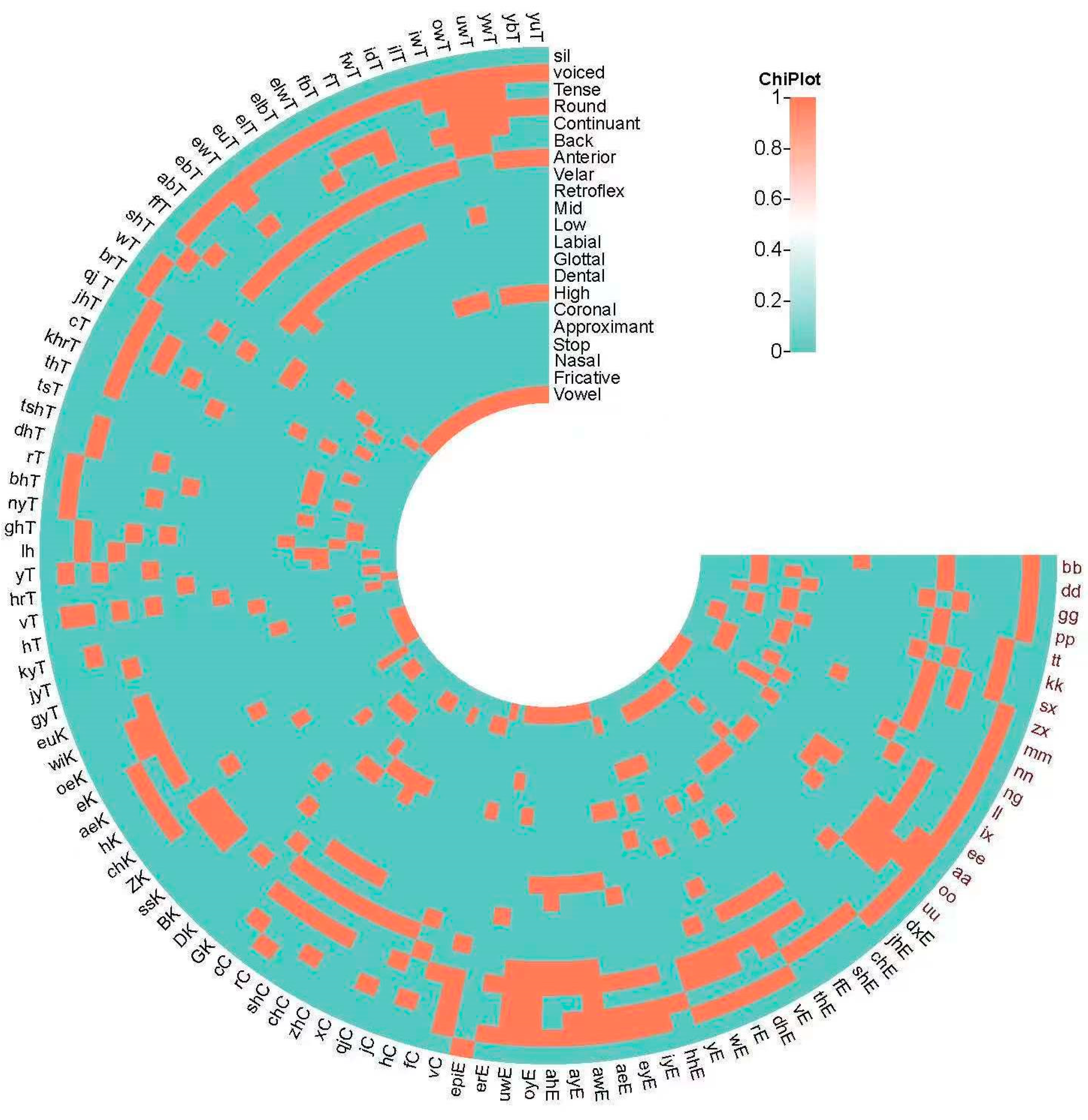
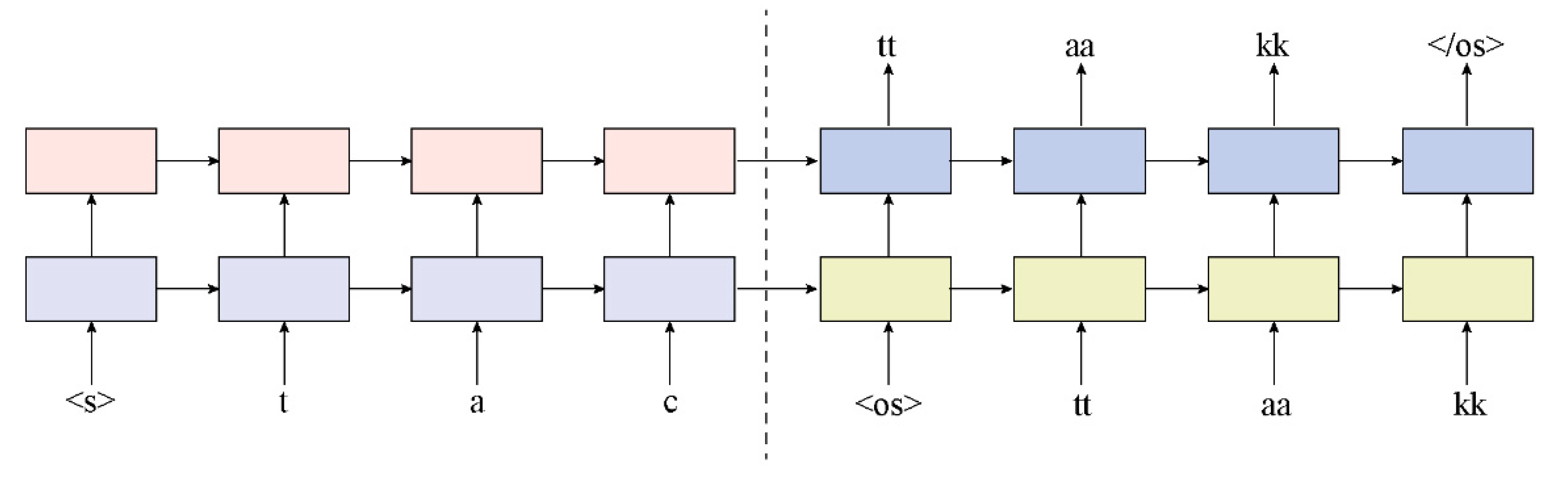
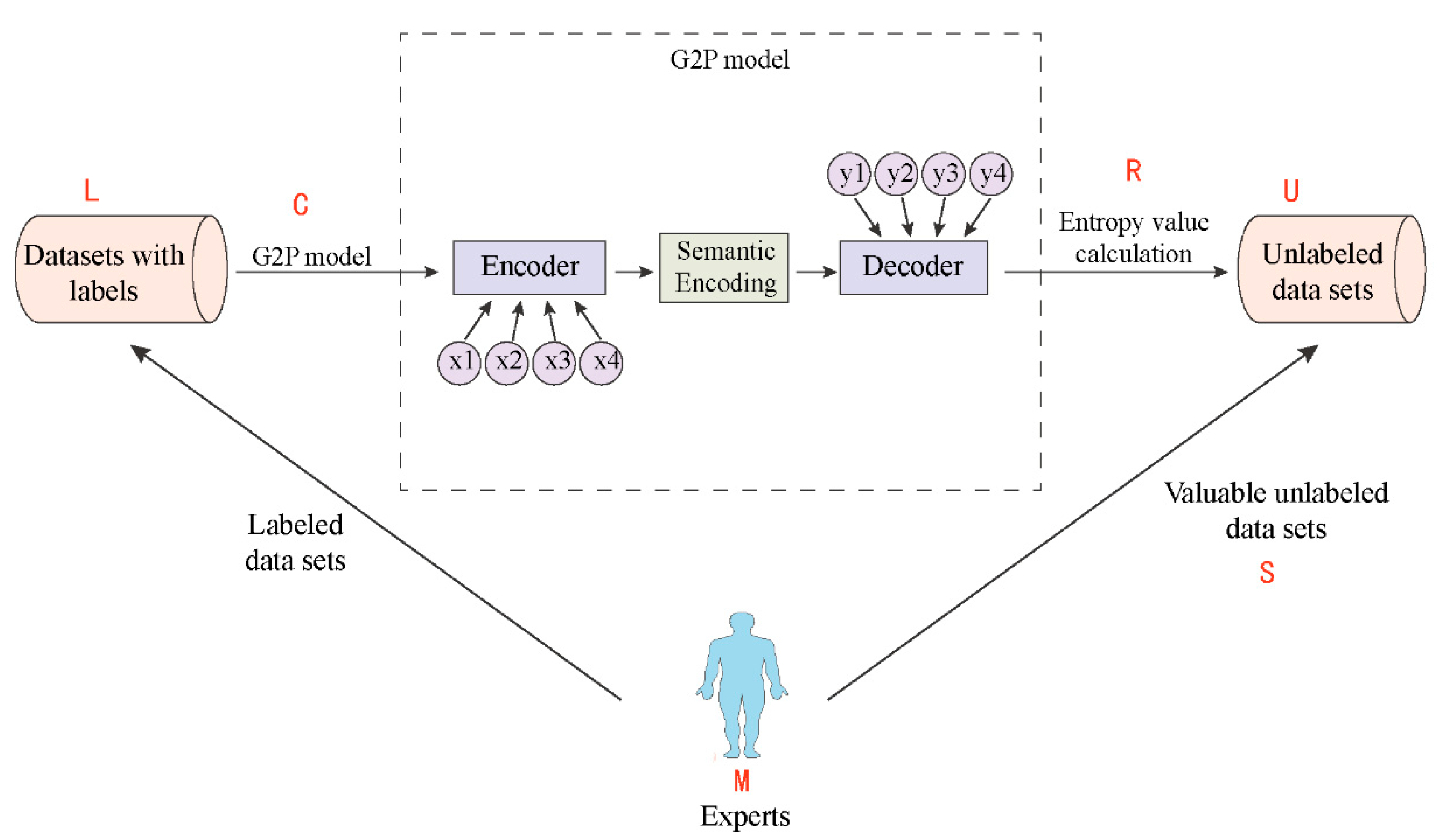
In this work, we used a grapheme-to-phoneme (G2P) model to predict phonemes for unannotated words, and obtained the predicted phonemes sequence along with the maximum probability of each predicted phoneme. To select the samples for labeling, we calculated the entropy value for each sample and ranked them in descending order. The sample with the highest entropy value, which has the greatest potential to improve the model, is then given to an expert for correction and labeling. By using a small number of high-value samples, our approach can improve model performance, greatly reduce the workload of expert labeling, and lower the construction cost of pronunciation dictionaries.
Assuming the grapheme sequence corresponding to sample k is [ x 1 , x 2 , , x n ] and the predicted probability vector corresponding to phoneme sequence is [ y 1 , y 2 , , y n ], the entropy value H k of sample k , is calculated by Equation (7).
H k = max ( y 1 ) l o g m a x ( y 1 ) + max ( y 2 ) l o g m a x ( y 2 ) + + max ( y n ) l o g m a x ( y n )
Calculate the probability vector y n for the predicted phoneme at location n by using Equation (8).
y n = s o f t m a x ( W h n )
W is the weight of the current hidden state h n .

4.4. Submodular Function

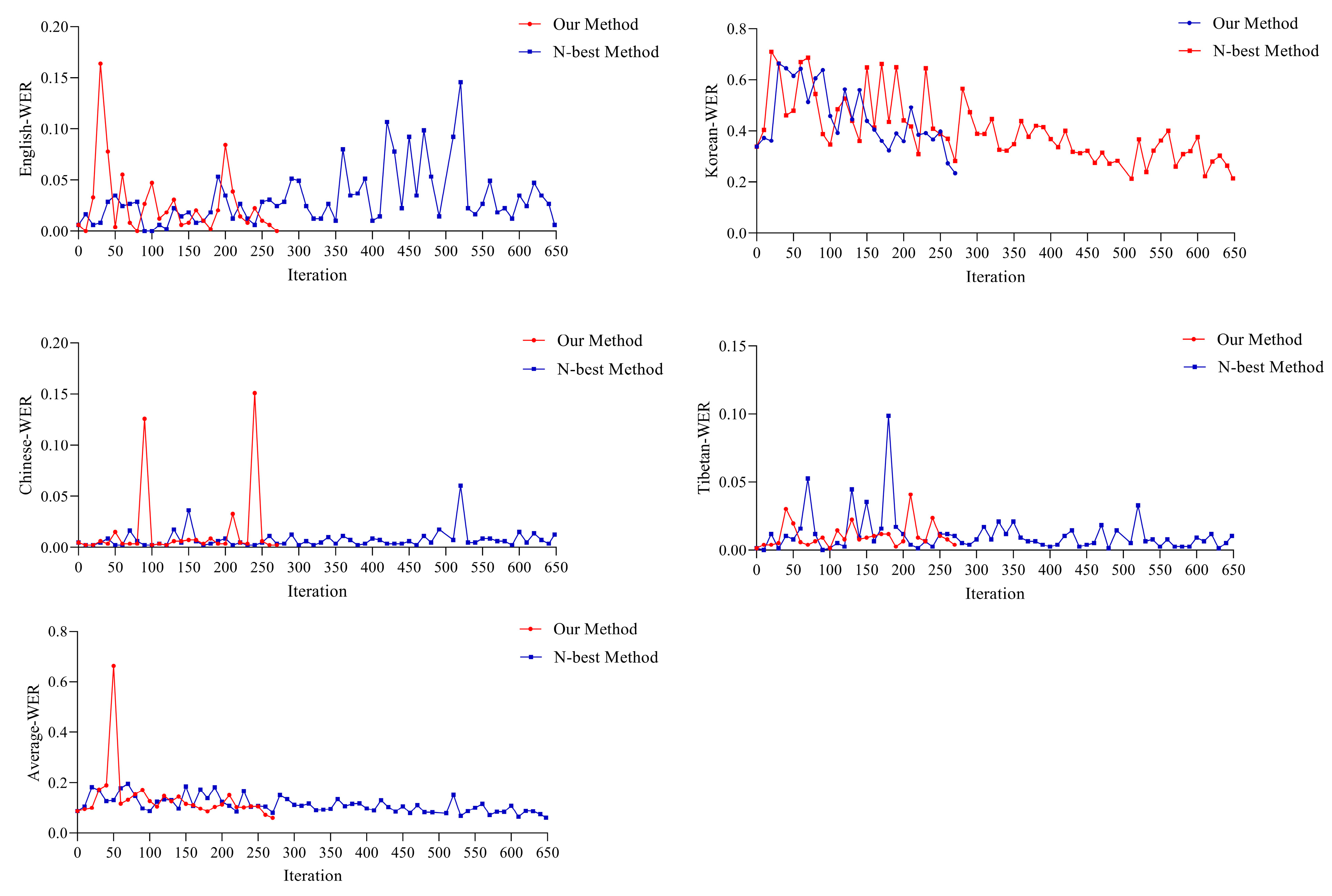
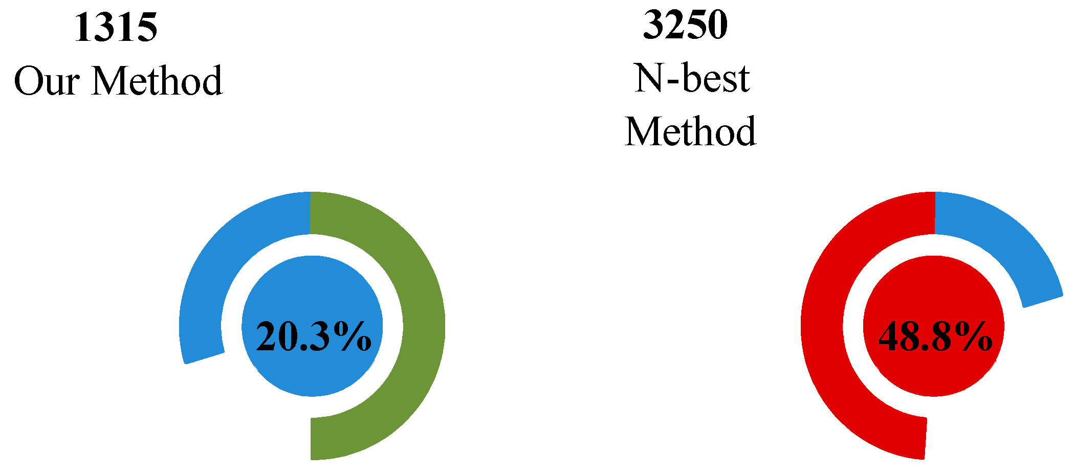
Most active learning methods select one valuable sample at a time for labeling, which is referred to as the non-batch method. However, this method is slow because the recognizer is retrained for each selected sample, and it cannot perform simultaneous multi-expert online labeling. In contrast, batch active learning methods can select multiple unlabeled samples at one time [32,33,34]. However, using only a single sample selection strategy in batch active learning can lead to poor results, as the selected samples may have a high information similarity (e.g., using the N-best method). To select the optimal subset of samples that represent the overall dataset, we optimized the sample selection problem using submodular function theory [35]. Specifically, we investigated the objective function of the near-optimal set of pronunciation dictionary samples and showed that our function had the submodularity property, which allowed for active learning so as to obtain a near-optimal subset of the corpus using a greedy algorithm. For the classifier, the goal of batch active learning is to form a set S of N unlabeled samples per iteration after user labeling, which is added to training set L . By retraining the classifier, the classifier can achieve the maximum performance improvement.
In active learning, the use of the maximum entropy principle as an evaluation criterion aims to select the most informative data to train the model and to achieve optimal results. This objective function can be represented as follows:
H ( Y S ) = p ( y ) l o g   p ( y | s )
In this equation, H ( Y | S ) quantifies the uncertainty of the target variable Y given a known set of variables S , using the concept of entropy. The probability distribution of the target variable y is denoted by p ( y ) , and p ( y | s ) represents the conditional probability distribution of y given a known set of variables s . The objective of this function is to maximize the uncertainty of the target variable   Y given a set of samples S . In the process, it is often necessary to select the next sample with the highest information content from a sample set [36]. The criterion for such a selection is to choose a sample that maximizes the uncertainty of the target variable Y , because this sample can provide the most informative new data that will facilitate a better understanding of the relationship between the target variable Y and the input variables. This, in turn, helps improve the performance of the model by enhancing its ability to learn from the data.
Regarding submodular functions, they are a special class of functions that possess important properties of monotonicity and diminishing marginal returns. In other words, function f satisfies the following two conditions:
1. Monotonicity: For any sets S _ 1 S _ 2 E and element, the function f satisfies the inequality f ( S _ 1 e ) f ( S _ 1 ) f ( S _ 2 e ) f ( S _ 2 ) .
2. Diminishing marginal returns: For any set S E and element e E S , the function f satisfies the inequality f ( S e ) f ( S ) f ( T e ) f ( T ) for any subset T S , such that T e S e .
Now, we will prove that the maximum entropy function H ( Y | S ) is a submodular function. Firstly, let us prove the monotonicity of   H ( Y | S ) . For any   S _ 1 S _ 2 E and element e E S _ 2 , we have:
H ( Y | S 1 e ) H ( Y | S 1 ) = p ( y ) l o g ( p ( y | S 1 e ) ) + p ( y ) l o g ( p ( y | S 1 ) ) = p ( y ) l o g ( p ( y | S 1 ) ) + p ( y ) l o g ( p ( y | S 1 e ) ) p ( y ) l o g ( p ( y | S 2 ) ) + p ( y ) l o g ( p ( y | S 2 e ) ) = H ( Y | S 2 e ) H ( Y | S 2 )
As the logarithmic function is a concave function, according to Jensen’s inequality, we have the following:
p ( y ) log ( p ( y | S 1 ) ) p ( y ) log ( p ( y | S 2 ) )
Therefore, we have the following:
H ( Y | S 1 e ) H ( Y | S 1 ) H ( Y | S 2 e ) H ( Y | S 2 )
Next, we prove that H ( Y | S ) satisfies the property of diminishing marginal returns. For any S E and element e E S , we need to prove the following:
H ( Y | S e ) H ( Y | S ) H ( Y | T e ) H ( Y | T )
where T S and T e S e .
According to the definition of   H ( Y | S ) , we have the following:
H ( Y S ) = p ( y ) l o g p ( y S )
Therefore, we can rewrite the above equation as follows:
p ( y ) l o g p ( y S e ) + p ( y ) l o g p ( y S ) p ( y ) l o g p ( y T e ) + p ( y ) l o g p ( y T )
Adding p ( y ) log p ( y | S T ) to both sides of the above equation, we obtain the following:
p ( y ) l o g p ( y S e ) + p ( y ) l o g p ( y S ) + p ( y ) l o g p ( y S T ) p ( y ) l o g p ( y T e ) + p ( y ) l o g p ( y T ) + p ( y ) l o g p ( y S T )
After simplification, we obtain the following:
p ( y ) l o g p ( y | S e ) p ( y ) l o g p ( y | T ) p ( y ) l o g p ( y | S T ) p ( y ) l o g p ( y | T e )
We decompose the exponents of each of the two terms on the right-hand side of the above equation as follows:
p ( y | S T ) p ( y | T e ) = p ( y | T ) p ( y | S e T ) p ( y | S e ) p ( y | T ) = p ( y | T e ) p ( y | S T e )
Substituting into the above equation, we obtain the following:
p ( y ) l o g p ( y S e ) + p ( y ) l o g p ( y T ) p ( y ) l o g   ( p ( y T ) p ( y S e T ) ) p ( y ) l o g   ( p ( y T e ) p ( y S T e ) ) )
By applying the concavity of the logarithmic function and Jensen’s inequality, we can obtain the following:
p ( y ) l o g p ( y | S e ) + p ( y ) l o g p ( y | T ) 2 p ( y ) l o g ( p ( y | T ) p ( y | S e T ) ) 2 p ( y ) l o g ( p ( y | T e ) p ( y | S T e ) )
As the function is convex, according to Jensen’s inequality, we have the following:
2 p ( y ) l o g ( p ( y | T ) p ( y | S e T ) ) p ( y ) l o g ( p ( y | T ) ) p ( y ) l o g ( p ( y | S e T ) )
Substituting into the above equation, we obtain the following:
p ( y ) l o g p ( y | S e ) + p ( y ) l o g p ( y | T ) p ( y ) log ( p ( y | T ) ) + p ( y ) log ( p ( y | S e T ) ) 2 p ( y ) l o g ( p ( y | T e ) p ( y | S T e ) )
Simplifying the above equation, we obtain the following:
H ( Y | S e ) H ( Y | S ) H ( Y | T e ) H ( Y | T ) I ( Y ; e | S T )
Therefore, we demonstrate that H ( Y | S ) is a marginally diminishing function. As H ( Y | S ) is a continuous function that satisfies the marginal diminishing property and range restriction, it is a submodular function.
In this way, we demonstrate that H ( S ) is a submodular function, allowing us to use a greedy algorithm for selecting an optimal subset of samples. Specifically, we can select the next sample to query by computing the marginal gain H ( Y | S e ) H ( Y | S ) for each element. We iteratively add elements to the sample set until the desired size is reached.

4.5. Near-Optimal Active Learning Algorithm

Starting from S = { } , the greedy algorithm was used to iteratively select the unlabeled dictionary corpa and add them to S until N dictionary corpa were added; then, the obtained set S was the near-optimal set. Algorithms 1 and 2 shows the near-optimal non-myopic active learning process and the greedy algorithm for finds S.
Algorithm 1 Near-optimal non-myopic active learning process
1. Randomly select a small number of unlabeled samples, assign a phoneme sequence to each of them, and add them into the training set L;
2. Train the model C on L;
3. Continue executing the following loop until the specified requirements have been satisfied;
  3.1 Greedily find S;
  3.2 Add S with true labels to L;
  3.3 Retrain the classifier C on L+S, and obtain its prediction accuracy on test date set;
Algorithm 2 greedy algorithm finds S
1. S = { } ;
2. W h i l e | S | N ;
2.1 Predict the annotation of each unlabeled sample in the dataset U \ ( L S )   based   on   the   current   identifier   C *   ( initially   C * = C ) .
2.2 Calculate the entropy value of the samples in the pre-labeled candidate set ac-cording to the entropy value calculation Formula (7) and rank them from highest to lowest according to the entropy value.
2.3 Add   the   pre - labeled   sample   k   with   the   largest   entropy   value   to   the   training   set   to   obtain   the   model   C k
2.4 Determine   whether   the   accuracy   of   C k   is   > C * ,   if   yes ,   execute   2.5 ,   otherwise   select   the   next   sample   and   execute   2.3  
2.5 S = S + s a m p l e   k
3. End

5. Experiments

5.1. Near-Optimal Active Learning Algorithm

The corpus preparation process involves several operations to ensure the quality and consistency of the data.
(1)
Filtering and sifting operations are performed to remove data with problems such as garbled codes and formatting errors, as well as phrases, sentences, or samples that do not constitute words.
(2)
A phoneme set normalization is performed to label all IPA phonemes in the original corpus with the corresponding phonemes of the common phoneme set.
(3)
A phoneme separation operation is performed to identify and separate each phoneme in the rewritten phoneme using a space character.
(4)
A de-duplication operation is performed to remove duplicate samples that have the same word form and pronunciation.
After sorting and filtering, a total of 9620 multilingual lexical data were annotated with the adapted common phoneme set phonemes, ensuring the quality and consistency of the data for further analysis.

5.2. G2P Experimental Results

In this paper, 9620 dictionary corpa in the pronunciation dictionary were divided into two parts—90% training data and 10% testing data for the G2P experiment. The results are shown in Table 3.
As shown in Table 3, the “word error rate (WER)” for Tibetan was 4.16%, indicating a satisfactory performance of the G2P model in the Tibetan script. However, some errors still existed. We focused on data for prediction errors, and the sources of error included ambiguity introduced by context, i.e., a lexeme with multiple valid phonemic interpretations. The WER for Chinese was 0.7%, which is an exceptionally low value that highlights the remarkable performance of the G2P model in the context of Chinese. This suggests a relatively straightforward mapping between Chinese characters and their phonemes. The WER for English is 13.96%, signifying more errors compared with other languages. Potential sources of errors encompass ambiguity in English spelling, where the same morpheme can have different pronunciations (e.g., “read” pronounced as “reed”, while “read” is pronounced as “red”). Irregularities in English pronunciation, where certain words deviate from typical phonetic patterns, also contribute to errors. The multi-language WER for Korean was 5.53%, indicating a moderate level of errors. Some potential sources of errors stemmed from the intricate phonetic rules in Korean, such as consonant assimilation or vowel harmony. Pronunciation ambiguity arises as pronunciation can vary based on context. The multilingual case (average WER across the four languages) was 6.2%. The average WER across different languages provides a holistic assessment. It is worth noting that distinct languages possessed varying features and grammatical rules, leading to noticeable differences in error distribution. However, this relatively low average value suggests a reasonably good performance of the G2P model across different languages.

5.3. Active Learning Experiments Results

In this paper, we used a self-built multilingual pronunciation dictionary dataset to evaluate a proposed approach for constructing multilingual pronunciation dictionaries based on near-optimal active learning. The dataset comprised 9620 words, with 1000 of them selected as the test data. We used 2000 of the remaining 8620 words as the initial training set for active learning, while the remaining 6658 words constituted the candidate set. The initial training set’s error rate in active learning was 6.2%. In the near-optimal active learning algorithm experiments, we selected N = 5 dictionary corpa each time from the unlabeled dataset and added them to the initial training set. We performed 263 iterations and selected 1315 data, and the WER reached 6.04%. To demonstrate the performance of the near-optimal active learning method, we compared the results with the N-best method of S. Tong et al. [14]. Figure 6 and Figure 7 show a comparison graphs of the G2P conversion accuracy of the two methods and the size of the samples selected. The N-best method selected the top five samples with entropy values, obtained their true labels, and added them to the training sets for retraining the model. The WER of the N-best method reached 6.07% after selecting 3250 data through 650 iterations. In Figure 7, the blue portion of our method on the left represented the percentage of the total data accounted for by the selected samples and the green portion represented the percentage of the remaining number, while the red portion of the N-best method on the right represented the percentage of the selected samples and the blue portion represented the percentage of the remaining data. The experimental results indicate that the near-optimal batch active learning method selected an unlabeled corpus with 20.3% of the total sample size, while the N-best method selected an unlabeled corpus with 48.8% of the total sample size. The results demonstrate that the proposed near-optimal active learning method outperformed the N-best method in terms of accuracy performance and the number of data selections.

6. Conclusions

Existing methods for constructing pronunciation dictionaries require an unusually large amount of data in order to be annotated by experts, which leads to a redundancy in the overall construction process. In this paper, we focused on the construction of multilingual pronunciation dictionaries and proposed an encoder-decoder based neural network as a G2P model for grapheme conversion. During the post-processing step of the trained G2P model, only samples with the highest information entropy were extracted, and a near-optimal active learning method was used for expert correction. The near-optimal active learning method proposed in this paper can achieve a high accuracy rate, even surpassing that of large-scale training data, using only a small number of valuable samples. As a result, the efforts required for expert labeling were significantly reduced, and the cost of constructing pronunciation dictionaries was also decreased.

Author Contributions

Conceptualization, Y.Z.; Methodology, D.C.; Software, D.C.; Validation, D.C.; Formal analysis, D.C.; Investigation, D.C.; Writing—original draft, D.C.; Visualization, Y.Z.; Supervision, Y.Z.; Project administration, L.W.; Funding acquisition, L.W. All authors have read and agreed to the published version of the manuscript.

Funding

This work was supported by funds as follows: (1) the National Natural Science Foundation of China (NSFC), “Research on end-to-end multi-task learning-based multi-dialect speech recognition method for Tibetan” (61976236); (2) the National Natural Science Foundation of China (NSFC), “Research on key technology of footplate water strider robot and its prototype development” (61773416); and (3) the Minzu University of China, “Research on Sino-Tibetan cross-language speech recognition method based on big data migration learning” (2020MDJC06).

Institutional Review Board Statement

This study does not involve human or animal research.

Informed Consent Statement

This study does not involve humans.

Data Availability Statement

This study chose not to publish the data, so if need the data, can contact the corresponding author.

Conflicts of Interest

The authors declare no conflict of interest.

Appendix A

1. Universal phonemes and their corresponding IPA values in our work.
Chinese PhonemesIPA ValuesKorean PhonemesIPA ValuesEnglish PhonemesIPA ValuesTibetan PhonemesIPA Values
aa[a]gg[k]bb[b]gyT[c]
oo[ɔ]GK[k̚] dd[d]jyT[nc]
ee[ɤ]nn[n]gg[g]kyT[cʰ]
ix[i]dd[t]pp[p]hT[h]
uu[u]DK[t̚]tt[t]vT[a:]
vC[y]ll[ɾ]kk[k]hrT[ʂ]
bb[p]mm[m]dxE[θ]yT[j]
pp[pʰ]bb[p]jhE[ʤ]kk[k]
mm[m]BK[p̚]chE[ʧ]ghT[ŋk]
fC[f]sx[s]sx[s]gg[kʰ]
dd[t]ssK[s͈] shE[ʃ]ll[l]
tt[tʰ]ng[ŋ]zx[z]lh[lʰ]
nn[n]zx[tɕ]fE[f]mm[m]
ll[l]ZK[tɕ̚]thE[ð]nn[n]
gg[k]chK[tɕʰ]vE[v]ng[ŋ]
kk[kʰ]kk[kʰ]dhE[ð:]nyT[ɳ]
hC[x]tt[tʰ]mm[m]pp[p]
jC[tɕ]pp[pʰ]nn[n]bhT[mp]
qC[tɕʰ]hK[h]ng[ŋ]bb[pʰ]
xC[ɕ]aa[a]ll[l]rT[r]
zhC[ʈʂ]aeK[ɛ]rE[r]sx[s]
chC[ʈʂʰ]ee[ʌ]wE[w]tt[t]
shC[ʂ]eK[e]yE[j]dhT [nt]
rC[ɻ]oo[o]hhE[h]tshT[ʈsʰ]
zx[ts]oeK[we]iyE[i]tsT[ʈʂ]
cC[tsʰ]uu[u]ix[ɪ]thT[ʈʰ]
sx[s]wiK[wi]ee[ɛ]khrT[ʈʂʰ]
ng[ŋ].euK[ɯ]eyE[aɪ]dd[d]
ix[i]aeE[æ]cT[tɕ]
aa[ɑ]jhT[ntɕ]
awE[ɔ]qj T[tɕʰ]
ayE[aɪ]brT[br]
ahE[ɑː]zx[nʈʂ]
oyE[ɔɪ]wT[w]
oo[aʊ]shT[ɕ]
uu[ʌ]ffT[f]
uwE[uː]aa[a]
erE[ɜː]abT[ʔ]
epiE[eɪ]ee[e]
ebT[eʔ]
ewT[e:]
euT[ȇ]
elT[Ɛ]
elbT[Ɛʔ]
elwT[Ɛ:]
fbT[øʔ]
fT[ø]
fwT[ø:]
ix[i]
idT[iʔ]
ilT[ĩ]
iwT[i:]
oo[o]
owT[o:]
uu[u]
uwT[u:]
ywT[y]
ybT[yʔ]
yuT[Ŷ]
2. Some sample results from our pronunciation dictionary in this work:
Tibetanཏུའངtt uu vT aa ng
Korean다른캐릭dd aa ll euK n2K kk aeK ll ix g2K
Chinese诗意shC ix ix
Englishbagbb aa gg

References

  1. Taylor, P. Hidden markov models for grapheme to phoneme conversion. In Proceedings of the Annual Conference of the International Speech Communication Association (INTERSPEECH), Brno, Czech Republic, 30 August–3 September 2021; pp. 1973–1976. [Google Scholar]
  2. Berndt, R.S.; Reggia, J.A.; Mitchum, C.C. Empirically derived probabilities for grapheme-to-phoneme correspondences in english. Behav. Res. Methods Instrum. Comput. 1987, 19, 1–9. [Google Scholar] [CrossRef]
  3. Mortensen, D.R.; Dalmia, S.; Littell, P. Epitran: Precision g2p for many languages. In Proceedings of the 11th International Conference on Language Resources and Evaluation (LREC), Miyazaki, Japan, 7–12 May 2018; pp. 2710–2714. [Google Scholar]
  4. Deri, A.; Knight, K. Grapheme-to-phoneme models for (almost) any language. In Proceedings of the 54th Annual Meeting of the Association for Computational Linguistics (ACL), Berlin, Germany, 7–12 August 2016; Volume 1, pp. 399–408. [Google Scholar]
  5. Sokolov, A.; Rohlin, T.; Rastrow, A. Neural machine translation for multilingual grapheme-to-phoneme conversion. In Proceedings of the Annual Conference of the International Speech Communication Association (INTERSPEECH), Graz, Austria, 15–19 September 2019. [Google Scholar]
  6. Peters, B.; Dehdari, J.; van Genabith, J. Massively multilingual neural grapheme-to-phoneme conversion. In Proceedings of the 1st Workshop on Building Linguistically Generalizable NLP Systems, Copenhagen, Denmark, 8 September 2017; pp. 19–26. [Google Scholar]
  7. Bisani, M.; Ney, H. Joint-sequence models for grapheme-to-phoneme conversion. Speech Commun. 2008, 50, 434–451. [Google Scholar] [CrossRef]
  8. Novak, J.R.; Minematsu, N.; Hirose, K. Wfst-based grapheme-to-phoneme conversion: Open source tools for alignment, model-building and decoding. In Proceedings of the 10th International Workshop on Finite State Methods and Natural Language Processing (FSMNLP), Donostia–San Sebastián, Spain, 23–25 July 2012; pp. 45–49. [Google Scholar]
  9. Rao, K.; Peng, F.; Sak, H.; Beaufays, F. Grapheme-to-phoneme conversion using Long Short-Term Memory recurrent neural networks. In Proceedings of the IEEE International Conference on Acoustics, Speech and Signal Processing (ICASSP), South Brisbane, Australia, 19–24 April 2015; pp. 4225–4229. [Google Scholar]
  10. Kirchhoff, K.; Bilmes, J.; Wei, K.; Liu, Y.; Mandal, A.; Bartels, C. A Submodularity Framework for Data Subset Selection; Technical Report AFRL-RH-WP-TR-2013-0108; University of Washington: Washington, DC, USA, 2013. [Google Scholar]
  11. Liu, Y.; Wei, K.; Kirchhoff, K.; Song, Y.; Bilmes, J. Submodular feature selection for high-dimensional acoustic score spaces. In Proceedings of the 2013 IEEE International Conference on Acoustics, Speech and Signal Processing, Vancouver, BC, Canada, 26–31 May 2013. [Google Scholar]
  12. Moore, R.C.; Lewis, W. Intelligent selection of language model training data. In Proceedings of the ACL 2010 Conference Short Papers, Uppsala, Sweden, 11–16 July 2010; pp. 220–224. [Google Scholar]
  13. Wu, Y.; Zhang, R.; Rudnicky, A. Data selection for speech recognition. In Proceedings of the 2007 IEEE Workshop on Automatic Speech Recognition & Understanding (ASRU), Kyoto, Japan, 9–13 December 2007; pp. 562–565. [Google Scholar]
  14. Tong, S.; Koller, D. Support vector machine active learning with applications to text classification. J. Mach. Learn. Res. 2001, 2, 45–66. [Google Scholar]
  15. Schohn, G.; Cohn, D. Less is More: Active Learning with Support Vector Machines. In Proceedings of the Seventeenth International Conference on Machine Learning (ICML 2000), San Francisco, CA, USA, 29 June–2 July 2000; pp. 839–846. [Google Scholar]
  16. Figueroa, R.L.; Zeng-Treitler, Q.; Ngo, L.H.; Goryachev, S.; Wiechmann, E.P. Active learning for clinical text classification: Is it better than random sampling? J. Am. Med. Inform. Assoc. 2012, 19, 809–816. [Google Scholar] [CrossRef] [PubMed]
  17. Hui, H.E.; Wang, J.-Y. Study of Active Learning Support Vector Machine and Its Application on Mongolian Text Classification. Acta Sci. Nat. Univ. NeiMongol 2006, 37, 560–563. [Google Scholar]
  18. Hoi, S.C.H.; Jin, R.; Lyu, M.R. Large-Scale Text Categorization by Batch Mode Active Learning. In Proceedings of the 15th International Conference on World Wide Web, Edinburgh, UK, 23–26 May 2006; Association for Computing Machinery: New York, NY, USA, 2006; pp. 633–642. [Google Scholar]
  19. Shen, D.; Zhang, J.; Su, J.; Zhou, G.; Tan, C.L. Multi-Criteria-Based Active Learning for Named Entity Recognition. In Proceedings of the 42nd Annual Meeting on Association for Computational Linguistics, Barcelona, Italy, 21–26 July 2004; Association for Computational Linguistics: New York, NY, USA, 2004; pp. 589–596. [Google Scholar]
  20. Tomanek, K.; Hahn, U. Reducing Class Imbalance during Active Learning for Named Entity Annotation. In Proceedings of the Fifth International Conference on Knowledge Capture, Redondo Beach, CA, USA, 1–4 September 2009; Association for Computing Machinery: New York, NY, USA, 2009; pp. 105–112. [Google Scholar]
  21. Shen, Y.; Yun, H.; Lipton, Z.C.; Kronrod, Y.; Anandkumar, A. Deep Active Learning for Named Entity Recognition. arXiv 2017, arXiv:1707.05928. [Google Scholar]
  22. Haffari, G.; Sarkar, A. Active Learning for Multilingual Statistical Machine Translation. In Proceedings of the Joint Conference of the 47th Annual Meeting of the ACL and the 4th International Joint Conference on Natural Language Processing of the AFNLP, Suntec, Singapore, 2–7 August 2009; Association for Computational Linguistics: Suntec, Singapore, 2009; Volume 1, pp. 181–189. [Google Scholar]
  23. Stüker, S.; Metze, F.; Schultz, T.; Waibel, A. Integrating multilingual articulatory features into speech recognition. In Proceedings of the Eighth European Conference on Speech Communication and Technology, Geneva, Switzerland, 1–4 September 2003; p. 10331036. [Google Scholar]
  24. Tong, S.; Garner, P.N.; Bourlard, H. Fast language adaptation using phonological information. In Proceedings of the Interspeech 2018, Hyderabad, India, 2–6 September 2018; pp. 2459–2463. [Google Scholar]
  25. King, S.; Taylor, P. Detection of phonological features in continuous speech using neural networks. Comput. Speech Lang. 2000, 14, 333–353. [Google Scholar] [CrossRef]
  26. Mikolov, T.; Kombrink, S.; Deoras, A.; Burget, L. Rnnlmrecurrent neural network language modeling toolkit. In Proceedings of the IEEE Automatic Speech Recognition and Understanding Workshop, Waikoloa, HI, USA, 11–15 December 2011. [Google Scholar]
  27. Hochreiter, S.; Schmidhuber, J. Long short-term memory. Neural Comput. 1997, 9, 1735–1780. [Google Scholar] [CrossRef] [PubMed]
  28. Lewis, D.D.; Gale, W.A. A sequential algorithm for training text classifiers. In Proceedings of the 17th Annual International ACM SIGIR Conference on Research and Development in Information Retrieval, Dublin, Ireland, 3–6 July 1994; Springer: New York, NY, USA, 1994; pp. 3–12. [Google Scholar]
  29. Guyon, I.; Cawley, G.; Dror, G.; Lemaire, V.; Statnikov, A. (Eds.) Challenges in Machine Learning. In Active Learning Challenge; Microtome Publishing: Brookline, MA, USA, 2011; Volume 6. [Google Scholar]
  30. Settles, B. Active Learning Literature Survey; Computer Sciences Technical Report 1648; University of Wisconsin-Madison: Madison, WI, USA, 2009. [Google Scholar]
  31. Sundermeyer, M.; Schluter, R.; Ney, H. Lstm neural networks for language modeling. In Proceedings of the InterSpeech, Portland, OR, USA, 9–13 September 2012; pp. 194–197. [Google Scholar]
  32. Joshi, A.J.; Porikli, F.; Papanikolopoulos, N. Multi-class active learning for image classification. In Proceedings of the IEEE Conference on Computer Vision and Pattern Recognition, Miami, FL, USA, 20–25 June 2009; pp. 2372–2379. [Google Scholar]
  33. Chattopadhyay, R.; Wang, Z.; Fan, W.; Davidson, I.; Panchanathan, S.; Ye, J. Batch mode active sampling based on marginal probability distribution matching. ACM Trans. Knowl. Discov. Data 2012, 2012, 741–749. [Google Scholar]
  34. Guo, Y.; Schuurmans, D. Discriminative batch mode active learning. In Proceedings of the International Conference on Neural Information Processing Systems, Vancouver, BC, USA, 3–6 December 2007; pp. 593–600. [Google Scholar]
  35. Zhao, Y.; Yang, G.; Xu, X.; Ji, Q. A near-optimal non-myopic active learning method. In Proceedings of the IEEE International Conference on Pattern Recognition, Tsukuba, Japan, 11–15 November 2012; pp. 1715–1718. [Google Scholar]
  36. Hoi, S.C.H.; Jin, R.; Lyu, M.R. Batch mode active learning with applications to text categorization and image retrieval. IEEE Trans. Knowl. Data Eng. 2009, 21, 1233–1248. [Google Scholar] [CrossRef]
Figure 1. The location of pronunciation dictionaries in ASR.
Applsci 13 09408 g001
Figure 2. Common phoneme sets and pronunciation features.
Applsci 13 09408 g002
Figure 3. The model structure of an encoder−decoder.
Applsci 13 09408 g003
Figure 4. Schematic diagram of LSTM encoder−decoder network.
Applsci 13 09408 g004
Figure 5. The active learning principle.
Applsci 13 09408 g005
Figure 6. Comparison of WER between the two methods.
Applsci 13 09408 g006
Figure 7. Comparison of the data selection between the two methods.
Applsci 13 09408 g007
Table 1. Generic pronunciation attribute table.
Pronunciation MannerVowel, Fricative, Nasal, Stop, Approximant, Continuant, Round, Tense, Voiced, Sil
Pronunciation positionCoronal, High, Dental, Glottal, Labial, Low, Mid, Retroflex, Velar, Anterior, Back
Table 2. Data samples.
WordGraphemeUniversal Phonemes
ChineseG U Ogg uu oo
Englishgog ogg oo
Tibetanསྨ སྨmm
Korean헤처ㅎ ㅔ ㅊ ㅓhK eK chK ee
Table 3. Experimental results.
Train DataTest DataEpochWER
Tibetan2331259204.16%
Chinese2592288200.7%
English10351152013.96%
Korean2700300205.53%
Multi-language8658962206.2%
Disclaimer/Publisher’s Note: The statements, opinions and data contained in all publications are solely those of the individual author(s) and contributor(s) and not of MDPI and/or the editor(s). MDPI and/or the editor(s) disclaim responsibility for any injury to people or property resulting from any ideas, methods, instructions or products referred to in the content.

