Abstract
A novel approach called the nonlinear convex decreasing weights golden eagle optimization technique based on a global optimization strategy is proposed to overcome the limitations of the original golden eagle algorithm, which include slow convergence and low search accuracy. To enhance the diversity of the golden eagle, the algorithm is initialized with the Arnold chaotic map. Furthermore, nonlinear convex weight reduction is incorporated into the position update formula of the golden eagle, improving the algorithm’s ability to perform both local and global searches. Additionally, a final global optimization strategy is introduced, allowing the golden eagle to position itself in the best possible location. The effectiveness of the enhanced algorithm is evaluated through simulations using 12 benchmark test functions, demonstrating improved optimization performance. The algorithm is also tested using the CEC2021 test set to assess its performance against other algorithms. Several statistical tests are conducted to compare the efficacy of each method, with the enhanced algorithm consistently outperforming the others. To further validate the algorithm, it is applied to the cognitive radio spectrum allocation problem after discretization, and the results are compared to those obtained using traditional methods. The results indicate the successful operation of the updated algorithm. The effectiveness of the algorithm is further evaluated through five engineering design tasks, which provide additional evidence of its efficacy.
1. Introduction
The earliest approaches to optimization problems were mathematical or numerical [1], where the goal was to arrive at a zero-derivative point to arrive at the final answer. The search space expands exponentially as the number of dimensions rises, making it nearly impossible to use these techniques to solve nonlinear and non-convex problems with many variables and constraints. Additionally, numerical approaches may enter local optimality when the derivative is also zero. Such numerical approaches cannot guarantee the discovery of a globally optimal solution, since real-world problems usually exhibit stochastic behavior and have unexplored search areas [2].
To overcome the limitations of numerical approaches, more sophisticated meta-heuristic algorithms are routinely utilized to address difficult optimization issues. These techniques have the benefits of being easily applied to continuous and discrete functions, not requiring any extra complicated mathematical operations such as derivatives, and having a low incidence of falling into local optimality points. Single-solution-based methods and population-based methods are the two categories of meta-heuristic techniques. A solution (typically random) is generated and iteratively improved until the stopping criterion is reached in single-solution-based methods. Based on the interaction of information between the solutions, population-based methods create a random set of solutions in a predefined search space and are iteratively updated to find the (near) optimal solution. Deep learning is also a form of optimization technique that is frequently used in many different fields [3].
The most prevalent metaheuristic algorithms are those that draw their inspiration from evolutionary theory or normal social animal behaviors like foraging, mating, hunting, memory, and other behaviors. To more efficiently look for portions of the problem that are viable, this strategy can be applied in several different ways. Numerous swarm intelligence systems serve as examples. Particle Swarm Optimization (PSO) [4] is the birthplace of swarm intelligence algorithms, which are inspired by birds’ foraging behavior. Ant Colony Optimization (ACO) [5] is an algorithm inspired by simulating the collective routing behaviors of ants in nature. Cuckoo Search (CS) [6] is an algorithm inspired by they raise their young using parasitism. Firefly Algorithms (FA) [7] are algorithms inspired by the flickering behavior of fireflies. Artificial Bee Colony (ABC) [8] is an algorithm inspired by imitating the honey collection mechanism of bees. New swarm intelligence algorithms have also been put forward in recent years. The Whale Optimization Algorithm (WOA) [9] is an algorithm inspired by the predatory behavior of whales. The Grey Wolf Optimizer (GWO) [10] is an algorithm inspired by the hunting behavior of grey wolf groups. The Seagull Optimization Algorithm (SOA) [11] is an algorithm inspired by simulating the migration of seagulls in the nature and the attack behavior (foraging behavior) in the migration process. The Slap Swarm Algorithm (SSA) [12] is an algorithm inspired by the aggregation behavior of slap swarms and their formation into a chain for predation and movement. The Butterfly Optimization Algorithm (BOA) [13] is an algorithm inspired by the behavior whereby butterflies receive, perceive and analyze the smell in the air to determine the food source and the potential direction of mating partners.
Algorithms for swarm intelligence do, however, inevitably have significant shortcomings. A number of variables have an enormous impact on the algorithm. This is because swarm intelligence systems usually need a lot of modifications, including with respect to population size, iterations, inertia weights, etc. The choice of these parameters has a considerable impact on the algorithm, because various problems necessitate different parameter values, which are difficult to regulate. Due to the dispersed nature of swarm intelligence algorithms, they must iterate repeatedly in order to discover the optimum solution, which slows down the algorithm. Simultaneously, the algorithm might enter a local optimum and continually look for an optimum in a small area that is not the best option, causing it to become stuck.
Researchers have recently presented some enhanced swarm intelligence algorithms and used them in various industries. Nafees et al. [14] proposed improved variants of Particle Swarm Optimization that incorporate novel modifications and demonstrate superior performance compared to conventional approaches in solving optimization problems and training artificial neural networks. A Fusion Multi-Strategy Marine Predator Algorithm for mobile robot path planning (FMMPA) was proposed by Luxian Yang [15]. A better marine predator algorithm (MPA-DMA) was proposed by Li Shouyu et al. [16], and it was used for feature selection with positive outcomes. However, the neighborhood clustering learning technique makes it simple to push the population beyond the cap, which is likely to have some bearing on how practical issues are resolved. A marine predator method based on mirror reflection urban and rural learning (PRIL-MPA), which was also applied in feature selection, was proposed by Xuming et al. [17]. In contrast to the previous method, in this article, an ideal person is identified to serve as a search guide for others, population variety is reduced, the search space is reduced, and local optimization is made simple. A marine predator algorithm (MSIMPA) combining chaotic opposition and collective learning, and which also offered the best individual guidance approach, was proposed by Machi et al. [18]. The issue remains the same, and group learning has the potential to result in extended running times, as well.
The use of cognitive radio has benefited from the work of numerous academics. The whale algorithm (IWOA) was enhanced by Xu Hang [19] and others to allocate the cognitive radio spectrum. The enhanced whale method outperforms competing algorithms thanks to a nonlinear convergence factor and a hybrid reverse learning strategy. Similar to this, the same authors enhanced the Grey Wolf Algorithm (IBGWO) [20] for usage in this field and employed three strategies: the nonlinear convergence factor, the Cauchy perturbation approach, and adaptive weight, achieving improved outcomes. Yin Dexin et al. [21] adopted a novel strategy in which the industrial internet of things was recognized as an environment, and applied the improved sparrow search algorithm (IBSSA) to the problem model. Similar to this, Wang Yi et al. [22] applied the enhanced mayfly algorithm (GSWBMA) to the cognitive heterogeneous cellular network spectrum allocation problem, offering helpful guidance for future researchers. Numerous researchers have also enhanced numerous swarm intelligence algorithms in the context of traditional engineering applications [23,24,25].
A novel algorithm called the golden eagle optimizer (GEO) [26] was put forward in 2021, which was motivated by two hunting behaviors of golden eagles. The cruising and attacking phases are changed in order to catch prey more quickly. The shift from the golden eagle’s cruise behavior to attack behavior has a direct impact on the end result. Cruise behavior mostly reflects the algorithm’s exploration function, while attack behavior primarily reflects the algorithm’s exploitation function. Because the original algorithm cannot balance the exploration and exploitation phases, it randomly switches from cruise behavior to attack behavior, which causes GEO to have a slow convergence speed, poor search accuracy, and weak robustness. There are some strategies to improve this. Few people, however, have previously used an improved approach to simultaneously take into account the cognitive radio allocation and traditional engineering design constraints, as described in this paper. Based on the advantages of the golden eagle approach, which include fewer optimization parameters, robustness to local optima, and superior handling of high-dimensional problems, this algorithm model is suggested.
This paper suggests a nonlinear convex decreasing weights golden eagle optimization technique based on a global optimization strategy to handle the problem. Arnold chaotic map initialization, nonlinear convex weight reduction, and a global optimization strategy make up the three components of the improved algorithm. An Arnold chaotic map with decent ergodicity is used to initialize the population of golden eagles in chaos maps. On the one hand, after examining several inertia weight types, nonlinear convex decreasing weights are utilized to help the golden eagle achieve improved convergence during the optimization process. On the other hand, in order to better achieve optimization, the golden eagle location update formula now includes the global optimization method, which connects each golden eagle to the generation’s most optimized individual. Under 12 benchmark functions and CEC2021, IGEO is contrasted with other sophisticated optimization algorithms to demonstrate its better performance. The results of the numerical experiment demonstrate that IGEO has better optimization performance than other techniques. Using a single-strategy method, we assess the numerical optimization abilities of the original GEO algorithm, IGEO, and GEO for 12 benchmark functions. The outcomes of the numerical experiment show how well these two methods function as compared to the original GEO. Eventually, IGEO is transformed into a binary algorithm and used for cognitive radio spectrum allocation. Compared with other improved algorithms, IGEO achieves higher spectral efficiency. Five classic engineering cases were also used to further test the performance of the algorithm.
The main contributions of this paper are as follows:
- (i)
- The Arnold chaotic map strategy is employed to help the golden eagle population obtain a better initial position.
- (ii)
- The nonlinear convex reduction strategy is used to coordinate the cruising and attacking behavior of the golden eagle, thereby improving its local and global search capabilities.
- (iii)
- The global optimization strategy is utilized to assist the golden eagle population in complex environmental optimization, enhancing the possibility of escaping from local optima.
- (iv)
- Twelve benchmark test functions and the CEC2021 test set are employed to assess the capabilities of the improved algorithm, including comparisons with eight other algorithms.
- (v)
- Various statistical tests, including the Wilcoxon rank-sum test and Friedman ranking, as well as Holm’s subsequent verification, are conducted to determine the overall ranking of the comparison algorithms and the improved algorithm on the twelve benchmark test functions and CEC2021, thereby validating the final performance of the algorithm.
- (vi)
- The individual effects of the nonlinear convex reduction strategy and the last global optimization strategy are tested separately.
- (vii)
- Algorithm complexity analysis is performed.
- (viii)
- The improved algorithm is applied to the classical problem of cognitive radio spectrum allocation and the results compared with those of commonly used algorithms.
- (ix)
- Five common engineering applications are utilized to test the search capabilities of the algorithm.
The following is a breakdown of this article. The second section goes over the fundamental ideas and the current state of GEO research. The third section offers a thorough explanation of the improved technique proposed in this article, and an analysis of its complexity. The fourth section, which mostly focuses on certain application components, contains simulation experiments and engineering best practices. In simulation experiments, there are compared experiments with a single improvement approach as well as comparative experiments between improved algorithms and alternative algorithms. The CEC2021 test set and 12 benchmark test functions served as the basis for these tests, and the experimental findings underwent statistical analysis. In engineering experiments, the enhanced algorithm is used to solve the well-known cognitive radio spectrum allocation problem, and the results compared with those of many other algorithms. Five classic engineering application cases are also used to verify the feasibility of the algorithm in this paper. Finally, the conclusions of this article are presented.
2. Related Works
2.1. Basic Work on GEO
2.1.1. Prey Selection
The exploration and exploitation phases make up the two sections of the GEO method. During the exploration phase, the golden eagle may be seen to fly around its target, before attacking it during the exploitation phase. As a result, each golden eagle must select a victim before cruising in and attacking it. Currently, the best solution is that which locates the prey. Every golden eagle is supposed to remember the best answer thus far. Each golden eagle hunts and flies in search of better prey. The golden eagle’s attack and cruise vectors are depicted in a two-dimensional trajectory diagram in Figure 1. Golden Eagle’s attack direction is shown by the left arrow, while its cruise direction is in-dicated by the downward arrow.
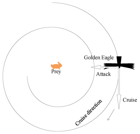
Figure 1.
Golden eagle’s cruise behavior.
2.1.2. Attack and Cruise
The procedure of catching the prey after the golden eagle gets close to it constitutes its attack behavior. A vector with a direction that goes to the prey and that extends from the golden eagle’s current location to the location of the prey in its memory can be used to replicate the attack behavior. Equation (1) can be used to describe how the golden eagle attacks.
where is the attack vector of the golden eagle, is the best position found by golden eagle so far, and is the current position vector of golden eagle .
The cruise behavior of the golden eagle is a process that starts with the eagle’s current location, turns around the prey, and continues to move toward the prey. In this procedure, the attack vector, the hyperplane, and the cruise vector are all connected. The cruise vector is in the tangent hyperplane of the golden eagle cruise trajectory, perpendicular to the assault vector. To compute the cruise vector, the hyperplane formula equation must first be obtained. A crucial reference plane in cruise behavior, the hyperplane is a linear subset with n − 1 dimensions in the n−dimensional linear space. An arbitrary point on the hyperplane and its normal vector can be used to identify it. Equation (2) displays the scalar form of the hyperplane equation in n−dimensional space.
where is the hyperplane’s normal vector, is a variable vector, and d is a constant. Therefore, for the arbitrary point of the hyperplane, Equation (3) can be deduced.
If the attack vector is regarded as a normal vector and the location of the eagle is regarded as an arbitrary point, Equation (4) can clearly be obtained.
The starting point of the cruise vector is the position of the golden eagle. The cruise vector can be chosen freely in n − 1 dimensions, but the hyperplane equation specifies the last dimension, as illustrated in Equation (4). There must be a free variable and a fixed variable, which are easy to determine using the following methods: randomly select a variable from among the variables as a fixed variable, denoted as ; and assign the random value to all variables except the variable. Therefore, the cruise vector of golden eagle in an n−dimensional space can be expressed using Equations (5) and (6).
where is the element of attack vector . The relationship between the golden eagle’s cruise behavior and attack behavior and the hyperplane is shown in Figure 2. A represents the Golden Eagle’s attack vector, while C represents a potential cruise vector for the Golden Eagle on this hyperplane.
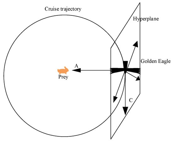
Figure 2.
The relationship between A, C and the hyperplane.
2.1.3. Move to New Location
The golden eagle cruises around the prey to obtain the cruise vector , and when it reaches an appropriate position, it pounces on the prey to obtain the attack vector . After the golden eagle has performed its cruise and attack, the displacement of golden eagle can be expressed as shown in Equation (7), while the position of golden eagle at the generation can be expressed as shown in Equation (8).
where and describe the random vector in [0,1], is the cruise coefficient and is the attack coefficient. and are the Euclidean norms of the cruise and attack vectors of golden eagle . is the old position of golden eagle at the generation, while is the new position of golden eagle at the generation. and can be calculated using Equation (9).
where and are ’s initial and final value, and are ’s initial and final value. and are the current and maximum generations, respectively.
2.2. Related Works on GEO
GEO is widely utilized by researchers, as it is an outstanding meta-heuristic method. Aijaz et al. [27] presented a two-stage photovoltaic residential system with electric vehicle charging capability, where the performance of the system was improved by an optimized proportional and integral gain selection bidirectional DC/DC converter (BDC) proportional–integral controller via the GEO algorithm. The golden eagle algorithm also outperformed the particle swarm and genetic algorithms in terms of performance. Magesh et al. [28] presented improved grid-connected wind turbine performance using PI control strategies based on GEO to improve the dynamic and transient stability of grid-connected PMSG-VSWT. In addition, GEO has also been applied to fuzzy control. Kumar et al. [29] set out to improve the performance of a nonlinear power system using a hierarchical golden eagle architecture with a self-evolving intelligent fuzzy controller (HGE-SIFC). GEO seems to be popular in wind and power systems. Sun et al. [30] accurately predicted wind power generation by means of the GEO algorithm, which they first improved, before proposing an extreme learning machine model that combined the improved GEO with an extreme learning machine for the prediction of wind power from numerical weather forecast data. In solar photovoltaic power systems, the GEO algorithm has another predictive feature. Boriratrit et al. [31] addressed the instability of machine learning and combined the GEO with a machine learning model, proposing a new machine learning model that yielded a smaller minimum root mean square error than the comparison model. Huge electricity demands have proved to be a tough challenge for power companies and system operators due to the increasing number of consumers in the electricity system and the unpredictability of electricity loads. Therefore, Mallappa et al. [32] proposed an effective energy management system (EMS) named golden eagle optimization with incremental electricity conductivity (GEO-INC) to meet demands with respect to load. Zhang et al. [33] proposed an improved GEO with improved strategies including an individual sample learning strategy, a decentralized foraging strategy and a random perturbation strategy, and these improved strategies were applied to a hybrid energy storage system with a complementary wind and solar power storage system for energy optimization. GEO has also been used in forecasting using learning machines; for example, a meta-learning extreme learning machine (MGEL-ELM) based on GEO and logistic mapping, and a same-date time-interval-averaging interpolation algorithm (SAME) [34] have been proposed in the literature to improve the forecasting performance of incomplete solar irradiance time series datasets. Profit Load Distribution (PLD) is a typical multi-constrained nonlinear optimization problem, and is an important part of energy saving and consumption reduction in power systems. Group intelligent optimization algorithms are an effective method for solving nonlinear optimization problems such as PLD. For the actual operational constraints of the power system in the PLD model, a novel GEO-based solution was proposed in [35]. A series of segmented quadratic polynomial sums were modelled for the fitness function as the cost function used to calculate the optimization by the first GEO. The results showed that the GEO was able to effectively solve the power system PLD problem. In addition to the prediction and power system aspects, GEO has also been applied in the field of image research. Al-Gburi et al. [36] applied GEO to the disc segmentation of human retinal images using pre-processing based on the golden eagle algorithm-guided geometric active Shannon contours and post-processing based on regular interval cross-sectional segmentation. Dwivedi et al. [37] proposed a novel medical image processing technique for analyzing different peripheral blood cells such as monocytes, lymphocytes, neutrophils, eosinophils, basophils and macrophages, using fuzzy c-mean clustering (MLWIFCM) based on GEO to perform cell nucleus segmentation. Justus et al. [38] proposed a hybrid multilayer perceptron (MLP)–convolutional neural network (CNN) (MLP-CNN) technique to provide services to SUs even under active TCS constraints in order to address the spectrum scarcity problem in cognitive radio. Eluri et al. [39] improved the GEO algorithm by using the transfer function to transform GEO into discrete space, and used time-varying flight duration to balance the cruise and attack parts of GEO. Moreover, their improved GEO was applied to feature selection, achieving good results. GEO has been used for multi-objective optimization in the context of the problem of reducing robot power consumption, obtaining a better Pareto frontier solution [40]. Xiang et al. [41] proposed PELGEO with personal example learning in combination with the grey wolf algorithm. Pan et al. [42] proposed GEO_DLS with personal example learning to enhance the search ability and mirror reflection learning to improve the optimization accuracy. Both PELGEO and GEO_DLS were applied for the 3D path planning of a UAV during power inspection. Ilango R et al. [43] proposed S2NA-GEO combined with a neural network learning algorithm. Later, a model for the uncertainty associated with renewable energy based on GEO was developed to relate the negative effects of variations in RES output for electric vehicles and intelligent charging [44].
2.3. Cognitive Radio Model
The demand for spectrum resources has significantly increased as a result of the quick expansion of wireless communication services brought on by the introduction of 5G communications. However, low spectrum utilization and the wastage of important resources have been caused by the fixed spectrum allocation mechanism and the limited supply of spectrum resources. In order to address these issues, Ghasemi et al. proposed Cognitive Radio (CR) [45] as a means to improve spectrum utilization.
Cognitive radio allows wireless communication systems to be aware of their surroundings, to secondarily utilize the unused spectrum holes of authorized users, to adapt to environmental changes and to automatically adjust system parameters, and to utilize the spectrum in a more flexible and efficient way. Existing spectrum allocation models include graph-theoretic coloring models [46,47], bargaining mechanism models [48], game theory models [49], etc.
Models for spectrum distribution can optimize system advantages, but it is challenging to precisely manage user fairness; therefore, they cannot guarantee the absence of flaws like those related to user fairness and unethical user competition. Scholars have used different swarm intelligence algorithms to optimize spectrum allocation, such as genetic algorithms (GA) [50], particle swarm algorithms (PSO) [4], butterfly optimization algorithms (BOA) [13], cat swarm algorithms (CSO) [51] and other intelligent optimization algorithms, for spectrum allocation problems in cognitive radio. Most of the above algorithms suffer from premature convergence, stagnation and iterative solution drawbacks when solving the problem. To overcome these problems and maintain population diversity, an improved golden eagle algorithm based on a graph-theoretic coloring model is applied to the optimization of the spectrum allocation model in this paper.
A conversion function is used to convert the search space from a continuous search space to a discrete search space. A suitable conversion function is required to increase the performance of the binary algorithm. Firstly, the conversion function is algorithm independent and does not affect the search capability of the algorithm; secondly, the computational complexity of the algorithm does not change. For continuous-to-discrete conversions, this work employs the Sigmoid function, which can be written as follows:
where is the position of the dimension in the individual in the golden eagle population at the generation.
The function of spectrum allocation is to build a reasonable allocation of available spectrum (channels) for cognitive users, which can satisfy the resource demand of cognitive users while effectively avoiding interference with primary users and maximizing the use of resources. Assuming that there are N secondary users (SUs) and M available channels in a certain region, the relevant definition of the graph-theoretic coloring model is as follows:
Theorem 1.
Idle matrix L , where indicates spectrum is available to SU and indicates spectrum m is not available to SU .
Theorem 2.
Spectrum efficiency matrix B , where is a positive real number representing the network benefit that SU can receive after obtaining spectrum .
Theorem 3.
Interference constraint matrix C , where represents individual user conflicts on the spectrum band, indicates that the simultaneous use of channel by SU and SU causes interference, while means no interference. When .
Theorem 4.
Non-interference allocation matrix A , where represents the final allocation strategy of M spectrums to N users, represents SU can use spectrum while represents cannot use. When .
Theorem 5.
Maximum total system benefit R .
Theorem 6.
Maximum percentage fairness fair .
3. Improved Golden Eagle Optimizer
3.1. Algorithm Model
3.1.1. Population Initialization Using the Arnold Chaotic Map
An individual golden eagle’s position is generated at random in the golden eagle optimization method. The existing population of golden eagles is relatively random and weak in terms of diversity, making it difficult to research and develop algorithms for algorithm optimization. In this paper, the initial location of the golden eagle is generated using an Arnold chaotic map to address the aforementioned issues. A Russian mathematician named Vladimir Igorevich Arnold suggested the Arnold chaotic map. This chaotic mapping technique can be used for repetitive folding and stretching transformation in a constrained space. The precise procedure is to first map the variables to the chaotic variable space using the cat mapping relationship, and then to use linear transformation to map the resulting chaotic variables to the space that needs to be optimized. Equation (11) describes the golden eagle’s starting position in the search space.
where and are the upper and lower bounds for variables, is the initial position of the golden eagle and Arnold is an Arnold chaotic map in the range of 0 to 1. The Arnold chaotic map has a simple structure and great ergodic uniformity. Its expression is shown in Equation (12).
3.1.2. Nonlinear Convex Decreasing Weight
The nonlinear convex decreasing weight represents the degree of inheritance of the current location. The algorithm has strong global optimization capability (i.e., better exploration) when this value is large, because the population individuals inherit a large portion of the particle positions from the previous generation, and the algorithm has strong local optimization capability when this value is small, because the population individuals inherit little (i.e., better exploitation). To balance exploration and exploitation, a nonlinear convex decreasing weight is added in GEO. The greater inertia weight enables the golden eagle to cruise and explore more effectively in earlier phases of GEO. Golden eagles can attack prey more effectively because of their reduced inertial weight in later stages of GEO. Equation (8) shows that the location and moving step of the previous generation determine the golden eagle’s updated position. In order for the previous person to affect the current individual, a nonlinear convex decreasing weight is added. Introducing the nonlinear convex declining weight is Equation (13).
where and are the initial and final weight values when the algorithm has gone through a number of iterations equal to the minimum and maximum numbers of generations, [ ] = [0.9 0.4]. t and T are the current and maximum generations. The different values of m represent the decreasing mode of inertial weight. Equation (14) represents the position update formula of the algorithm after introducing nonlinear convex decreasing weight.
The value of m influences the weight’s decreasing mode and further impacts the algorithm’s performance during optimization, most notably its rate of convergence. Figure 3 depicts the nonlinear convex decreasing weight when m rises from 1 to 7. The following tests are conducted to investigate the value of m that is most advantageous to the algorithm. Six benchmark functions are chosen as experimental objects, 30 unique experiments are carried out, and seven different m values explain seven algorithms. The evaluation was conducted after generating the average convergence curve for these six benchmark test functions. The precise method involves finding the smallest number of iterations for each of the seven methods under the conditions of best convergence accuracy. The algorithm with the fewest iterations receives seven points, and so on, until the algorithm with the most iterations, which receives one point. The results of the seven algorithms for the six benchmark test functions are displayed in Table 1. Figure 3 and Table 1 show that the lowest score for m = 1, which reflects the linearly decreasing inertia weight, shows the algorithm’s slowest convergence pace. In this paper, the value of m is chosen to be 4, because it has the highest score. It also exhibits the fastest convergence speed.
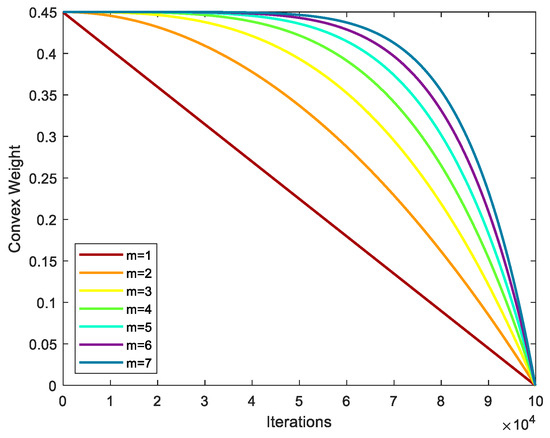
Figure 3.
Different degrees of nonlinear convex decreasing weights.

Table 1.
The influence of different values of parameter m on the algorithm.
3.1.3. Global Optimization Strategy
Without significant social contact, the golden eagle’s position update formula in the golden eagle optimization method simply refers to the historical memory of the golden eagle’s position and move step from the previous iteration. Such a blind random search in space not only fails to speed up the population’s search, but also frequently hinders its ability to swiftly identify the best option. The golden eagle position update formula is enhanced by the introduction of a global optimization strategy. For each iteration, the best-fitting individual in the population is picked so that it can interact with the current individual and quickly find the ideal solution. The improved formula is shown in Equation (15).
where and are random numbers between 0 and 2. is the best global position of the golden eagles.
3.2. Detailed Steps for the Improved Golden Eagle Optimizer Algorithm
The three strategies mentioned above can significantly increase the algorithm’s convergence speed and search precision, balance global exploration with local exploitation, and improve the performance of the original GEO. The IGEO implementation method is depicted in Figure 4, and Algorithm 1 presents the pseudo-code for the suggested IGEO. The Golden Eagle’s ideal hunting position is depicted in Figure 4 by .
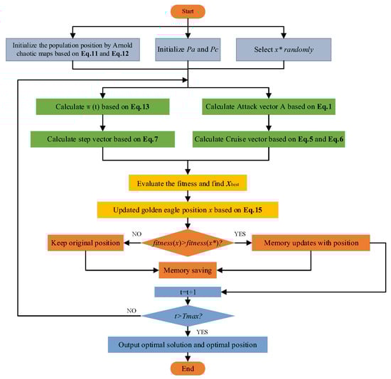
Figure 4.
Flowchart of the improved golden eagle optimizer algorithm.
The pseudo-code of the proposed IGEO is shown in Algorithm 1.
| Algorithm 1 Pseudo-Code of IGEO |
| Setup 1 Set the population size N, current iterations t = 0 and maximum generations T = 1000 |
| 2 Initialize the population position by Arnold chaotic map |
| 3 Evaluate fitness function |
| 4 Initialize other parameters: Pc and Pa and golden eagle’s memory |
| 5 While t < T |
| 6 Update Pc and Pa based on Equation (9) |
| 7 For i = 1:N |
| 8 Calculate A based on Equation (1) |
| 9 If the length of A is not equal to zero |
| 10 Calculate C based on Equations (5) and (6) |
| 11 Calculate ω(t) based on Equation (13) |
| 12 Calculate based on Equation (7) |
| 13 Calculate the population fitness and selected fitness optimal individual xbest |
| 14 Update new position xt+1 based on Equation (15) and calculate its fitness |
| 15 If fitness(xt+1) is better than fitness of position in golden eagle’s memory |
| 16 Replace the new position with position in golden eagle’s memory |
| 17 End If |
| 18 End If |
| 19 End For |
| 20 End While |
3.3. Algorithm Complexity Analysis
The running process of the IGEO is mainly divided into the following two parts: population initialization and the algorithm main cycle. For the initialization part, the Arnold chaotic map is used to initialize the golden eagle population. N golden eagles are initialized in the D dimension, with a complexity of O (N × D). In the main part of the algorithm, for the boundary setting of N golden eagle individuals, the complexity is O (N). In the golden eagle location update formula, the complexity is O (N × D). For the whole main loop part, there are T iterations, so the algorithm complexity of the whole main loop part is O (N) + O (N × D) + O (N × D × T). Therefore, the total complexity of the entire algorithm is the sum of the complexity of the initialization part and the complexity of the main loop part, which is O (N × D × T). The complexity of the improved algorithm is not more complex than the original, but the optimization effect is much better.
4. Analysis of Experimental Results
4.1. Simulation Experiment
4.1.1. Experimental Settings and Test Functions
The experimental operating environment was made up of the Windows 10 64-bit operating system, an Intel(R) Core (TM) i5-7200U processor, 2.5 GHz main frequency, and 4.00 GB of RAM. The algorithm was created using MATLAB 2021a as a basis.
Experiments were conducted on 12 benchmark functions in order to confirm the usefulness of the IGEO in solving diverse optimization challenges. Two continuous unimodal benchmark functions (F1 and F2) were used to assess the algorithm’s speed and accuracy of convergence. To assess the algorithm’s ability to perform a global search and the likelihood of leaving the local optimum, six complex multimodal benchmark functions (F3–F8) were utilized. The comprehensiveness of the approach was assessed using four fixed low-dimensional benchmark functions (F9–F12). Table 2 displays the specifications of the benchmarking functions.
Table 2.
Benchmark test functions information.
4.1.2. Comparative Analysis of Performance with Other Algorithms
In order to verify the overall performance of the IGEO, eight algorithms were selected for comparison, including the butterfly optimization algorithm (BOA) [13], the grey wolf optimizer (GWO) [10], particle swarm optimization (PSO) [4], the sine cosine algorithm (SCA) [52], the slap swarm algorithm (SSA) [12], the whale optimization algorithm (WOA) [9], the golden eagle optimizer algorithm (GEO) [26], and the golden eagle optimizer with double learning strategies (GEO_DLS) [42]. To ensure fairness, the population number for all algorithms was 50, and the maximum number of iterations was 1000. In addition, the parameters of each original algorithm were the best, as shown in Table 3.
Table 3.
Parameter settings of each algorithm.
Table 4 displays the analytical results in relation to the other eight algorithms, along with the mean, standard deviation (std), and average running time. These results show the accuracy of the convergence and optimization of the algorithms. From the results for mean value and standard deviation, it can be seen that IGEO has the best search accuracy: the IGEO was able to readily obtain an excellent advantage that could be matched by no other algorithm on F1, F2, F4, F5, F7, F8, and F11, and the only other algorithms that achieved the same grades as IGEO were GEO_DLS on F3, WOA on F6 and F9, GWO on F10, and PSO on F12.
Table 4.
Test results for the comparison of IGEO and other advanced algorithms.
The performance on the continuous unimodal functions F1–F2 demonstrate the superior optimization capabilities of IGEO. The performance on the challenging multivariate functions (F3–F8) demonstrates IGEO’s capacity to avoid local maxima. Only WOA on F6 and GEO_DLS on F3 have an optimization precision as good as IGEO. Last but not least, IGEO’s performance on the fixed low-dimensional functions F9–F12 demonstrates its all-encompassing capabilities. Unfortunately, IGEO’s performance in this area is marginally subpar: the optimization accuracy of WOA on F9, GWO on F10, and PSO on F12 are all equal to that of IGEO. Due to the characteristics of the method itself, GEO, GEO_DLS, and IGEO have the longest mean running times, while IGEO performs the best overall.
An MAE ranking [53] on the best outcomes of 50 experiments was performed in this work in order to more accurately assess the optimization performance of each method on the test function.
In a quantitative analysis of all algorithms, the average absolute error of 12 benchmark functions is used to rank all algorithms. The algorithm’s performance increases as MAE decreases. The formula for determining the MAE ranking of these benchmark functions is given in Equation (16), and Table 5 displays the ranking of these algorithms.
where is the number of benchmark functions, is the average of the optimal results generated by the algorithm, and is the corresponding theoretical optimal value.
Table 5.
Comparison of MAE ranking between IGEO and other advanced algorithms.
Table 5 shows that IGEO has the lowest MAE value and the best performance.
In Figure 5, the average convergence curve is also presented in logarithmic form for a better and more precise comparison of the experimental data. The absolute values of all findings are plotted, because −1 is the ideal value of the function F8.
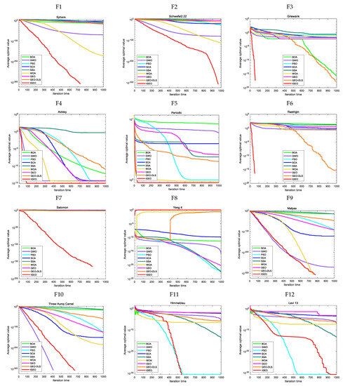
Figure 5.
IGEO and other algorithms’ convergence curves on the test functions.
In Figure 5, the test results for the convergence speed and search accuracy of the algorithms are presented. The results demonstrate that IGEO outperforms the comparison algorithms on F1 to F8. Specifically, for F1, F2, F3, F6, and F7, IGEO shows significant advantages in terms of average value, indicating an overwhelmingly high convergence speed and search accuracy. For F4, F5, and F8, IGEO exhibits better performance than the comparison algorithms, and the ability to accurately capture the theoretical optimal values of 0.9 and −1 for F5 and F8, respectively. While IGEO shows inferior performance on F9, F10, F11, and F12, its standard deviation is 0, demonstrating superior robustness compared to other algorithms. Regarding F9, IGEO’s performance is second only to WOA. The convergence speed of GWO and the search accuracy of WOA on F9 are comparable to those of IGEO. For F10, GWO outperforms both IGEO and WOA in terms of performance. For F11 and F12, although the average convergence curves of PSO and IGEO are similar, the results presented in Table 4 clearly indicate that IGEO exhibited a higher search accuracy than PSO.
Table 4 and Figure 5 present the optimization results for the benchmark functions F1 to F8 in general dimensions (dim = 30), where it is evident that IGEO achieved the best results in terms of both convergence speed and search accuracy. To verify the comprehensive performance and robustness of IGEO, experiments were conducted on the eight benchmark functions under 100-dimensional conditions using the comparison algorithms. The conditional parameters of each algorithm were consistent with those shown in Table 3, and each algorithm was independently run 50 times for each function. Table 6 presents the results of the comparison with the other seven original algorithms, including mean and standard deviation (std). Table 6 clearly demonstrates that IGEO outperformed the other algorithms in terms of both average value and standard deviation, indicating its superior exploration and exploitation ability.
Table 6.
Comparison of the test results of IGEO and other advanced algorithms (dim = 100).
Here, the optimization outcomes for the CEC2021 test set are also displayed to further demonstrate IGEO’s efficacy. Recent winners are contrasted with IGEO. Both traditional improvements to particle swarm optimization, such EIW_PSO [54], and advances in new swarm intelligence algorithms, like FMMPA [15], are included among the comparison algorithms. Additionally, IGEO is contrasted with upgraded GEO algorithms, including GEO_DLS [42], CMA-ES-RIS [55], and L-SHADE [56]. Table 7 displays the specific outcomes. The data in the table were derived by deducting these values, because none of the 10 functions in the CEC2021 test set have an ideal value of 0. The table includes the minimum value, maximum value, standard deviation, and average value of the algorithm optimization. The table shows that IGEO’s performance is still fairly strong, overall, despite the fact that it is not the best for every function.
Table 7.
Comparison of IGEO and other comparison algorithms on CEC2021.
4.1.3. Statistical Significance Testing
In this work, the Wilcoxon statistical test and the Friedman test are performed on the best results of the 50 experiments, and further follow-up verification was conducted using the Holm method to more accurately evaluate the optimization performance of each method on the test function.
- (i)
- Wilcoxon test for statistics. If IGEO obtains the best results, it is then evaluated against the eight comparison algorithms using the rank-sum test, which is carried out at the 5% significance level. The best results from 50 separate tests make up the data vectors for comparison.
When p is less than 5%, the original hypothesis cannot be ruled out at a significance level of 100 × 5%, indicating that the enhanced algorithm produces better results than the comparison algorithm does, and vice versa. Table 8 displays the rank-sum test p values for each algorithm. Among these, “NAN” denotes that the numerical comparison is irrelevant and that the ideal value of the two procedures is 0. “+”, “−”, and “=” signify that IGEO’s performance is better than, worse than, or equal to that of the comparison algorithm, respectively.
Table 8.
Comparison of rank-sum test values between IGEO and other advanced algorithms.
Table 8 shows that when compared to the original algorithms GEO and SSA, IGEO achieves a 100% optimization rate; when compared to BOA, PSO, and SCA, IGEO achieves a 91.2% optimization rate; and when compared to GWO, WOA, and GEO DLS, IGEO achieves an 83.3% optimization rate. These results illustrate IGEO’s thorough performance across the 12 benchmark functions.
- (ii)
- Friedman Test. A differential analysis technique called the Friedman test can be used to solve issues by combining various approaches. The advantages and disadvantages of the algorithms are compared by computing the average ratings of the algorithms being compared. With this approach, in contrast to the rank-sum test approach, the comparison algorithm’s overall performance can be further assessed. The formula for the Friedman test is as follows:
where denotes the algorithm’s final ranking, denotes the quantity of the test functions, and denotes the ranking of algorithm in the test function . Using Equation (17), the Friedman rankings for the benchmark functions and CEC2021 are determined, and the results obtained are reported in Table 6 and Table 7. To solve the algorithm ranking in a specific test function fairly, an average of 30 separate runs is used. Table 9 shows that IGEO’s comprehensive rating comes in top place. In addition, Table 10 shows that IGEO ranks lower than FMMPA.
Table 9.
Friedman ranking under benchmark function comparison.
Table 10.
Friedman ranking under CEC2021 comparison.
- (iii)
- Holm verification. Table 11 and Table 12 present the data acquired after further Holm verification of the results by comparing the results obtained with the original and improved algorithms. Assuming that each algorithm’s distribution is equal to that of the classical original algorithm, the system uses Friedman to perform a bidirectional rank variance analysis on the pertinent samples at a significance level of 0.05.
Table 11. Subsequent Holm verification results for all algorithms under the benchmark testing functions.
Table 12. Subsequent Holm verification results for all algorithms under CEC2021.
After further verification usign Holm, the average chi square value after testing is 34.296, the critical chi square value of the system is 15.507, the degree of freedom gained through data testing is 9, and the p-value is significantly below 0.05. The original presumption is disproved, i.e., the presumption that all optimization results follow a uniform distribution. Table 11 demonstrates that the WOA, GEO_DLS, PSO, and GWO models reject the null hypothesis and significantly deviate from the enhanced method. SCA, BOA, GEO, and SSA all support the initial theory and differ little from the initial method. The final order of preference for the algorithms is IGEO > WOA > GEO_DLS > PSO > GWO > SCA > BOA > GEO > SSA.
Similarly, in the experiment using CEC2021 as the test object, the critical chi square value of the system is 19.943, which therefore also rejects the original hypothesis. Table 12 demonstrates that the L-SHADE, GEO_DLS, CMA-ES-RIS and FMMPA models reject the null hypothesis and significantly deviate from the enhanced method. Only EIW_PSO rejects the hypothesis that there is a significant difference from IGEO. The final order of preference for the algorithms is FMMPA > IGEO > L-SHADE > GEO_DLS > CMA-ES-RIS > EIW_PSO.
4.1.4. Comparative Analysis of Different Strategy Algorithms
To explore the effectiveness of the proposed algorithm and study the impact of different strategies on the golden eagle optimizer algorithm, ablation experiments were conducted. GEO with a single strategy includes GEO with nonlinear weights (wGEO) and GEO with global optimization strategy (pGEO). The experimental parameter settings were consistent with those presented in Table 3. The experimental algorithms included GEO, wGEO, pGEO, and IGEO. Each algorithm was independently run 50 times on each of the 12 test functions selected in this article. The experimental results are presented in Table 13.
Table 13.
Comparison of test results for IGEO and various single-strategy algorithms.
The results presented in Table 13 indicate that the optimization accuracy when using a nonlinear convex decreasing weight strategy or a global optimization strategy individually is inferior to that when using the mixed strategy, with a significant difference in optimization accuracy despite having the same running time. For F1, F2, F7, F9, and F11, IGEO demonstrated absolute superiority, achieving the highest optimization accuracy. For F3 to F6, wGEO, pGEO, and IGEO exhibited similar search accuracy, which was significantly better than that of GEO. For F8, F10, and F12, pGEO and IGEO exhibited similar performance.
To verify the performance of IGEO in terms of convergence speed and search accuracy, Figure 6 presents the average convergence curves of the benchmark functions. Similarly, since the optimal value of function F8 is −1, the absolute value of all results is taken when drawing the visualization. Compared with wGEO and pGEO, IGEO exhibits faster convergence on F3 to F6, although the convergence precision is the same. IGEO and pGEO achieve identical performance on F8. For F10 and F12, IGEO demonstrates a slight advantage in terms of convergence speed, while the average optimal value and standard deviation are close to the theoretical optimal value. Furthermore, IGEO performs optimally on the other functions.
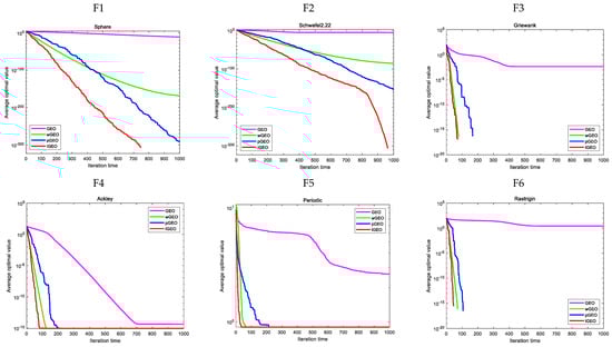
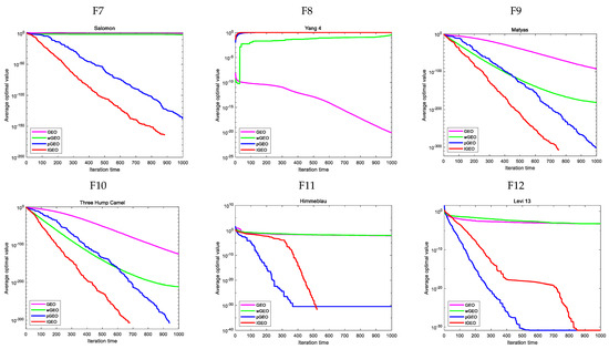
Figure 6.
IGEO and various single−strategy algorithms’ convergence curves on the benchmark functions.
Combining the exploration of the value of m described in Section 3.2 and the two numerical experiments reported in Section 4.1.2 and Section 4.1.3, it can be concluded that the nonlinear convex decreasing weight mainly affects the convergence speed of the algorithm, indicating the algorithm’s ability to perform exploration. Conversely, the global optimization strategy mainly affects the search accuracy of the algorithm, indicating the algorithm’s ability to perform exploitation. In this article, these two capacities are effectively balanced by combining these two strategies to improve GEO, leading to improved algorithm performance. The theoretical numerical experiment for the revised algorithm is presented in this section. In Section 4.2 and Section 4.3, specific application experiments are provided.
4.2. Cognitive Radio Application
4.2.1. IGEO Problem Solving Model
In the proposed model for solving the spectrum allocation problem, each golden eagle’s binary-coded position represents a feasible spectrum allocation strategy. To determine the optimal spectrum allocation scheme, it is necessary to solve the interference-free allocation matrix to maximize the total system benefit. Based on the status of the secondary user (SU) utilizing the channel in the idle matrix , SU n cannot utilize channel m. Consequently, matrix in the corresponding position must be zero. Conversely, if , then can be either 0 or 1. The processing strategy proposed in the literature [45] for the idle matrix involves exclusively numbering those elements for which the array is 1. Furthermore, the number of elements in matrix that equal 1, representing the coding length D of the golden eagle individuals, is recorded. The formula for calculating this is as follows:
Figure 7 illustrates the mapping relationship between the location encoding and the assignment matrix. In the current cognitive wireless network environment, assuming N = 6 cognitive users and M = 4 channels, the idle matrix is calculated based on the network topology. The locations of 1 in matrix are identified, and the location x of an individual golden eagle’s binary encoding is mapped to the allocation matrix in increasing order.
Figure 7.
Mapping association between position coding and allocation matrix.
The pseudo-code of the proposed IGEO solving CR when applying IGEO to the cognitive radio model is shown in Algorithm 2.
| Algorithm 2 Pseudo-Code of IGEO for Solving CR |
| 1 Initialize the idle matrix L, the benefit matrix B, the non-interference distribution matrix C |
| 2 Calculate the number of values in L, and then enter the appropriate values of n and m at the position of 1 in the idle matrix L. Find the dimensions D of the optimization problem, which corresponds to the number of unique golden eagle codes, by listing the position elements in an increasing order of n and m |
| 3 Set algorithm parameters N, t = 0, T = 1000 |
| 4 Initialize Arnold chaotic map |
| 5 According to the problem dimension D, the number N, and Arnold map, the individual position is initialized, and the golden eagles’ position is mapped to the allocation matrix A. |
| 6 If all n and k in the coherence matrix satisfy the condition , the values of and in the assignment matrix A are both 1. |
| 7 Set one of them to 0 and keep the other unchanged |
| 8 End If |
| 9 The binary coding corresponding to the golden eagle individual after processing the non-interference constraint matrix |
| 10 According to the distribution matrix A and the benefit matrix B, the individual fitness value is calculated. |
| 11 Initialize other parameters: , and golden eagle’s memory |
| 12 While t < T |
| 13 Update and based on Equation (9) |
| 14 For i = 1:N |
| 15 Calculate A(attack vector) based on Equation (1) |
| 16 If the length of A is not equal to zero |
| 17 Calculate C based on Equations (5) and (6) |
| 18 Calculate ω(t) based on Equation (12) |
| 19 Calculate based on Equation (7) |
| 20 Calculate the population fitness and selected fitness optimal individual xbest |
| 21 Update new position xt+1 based on Equation (14) and calculate its fitness |
| 22 Discretize the current position of the golden eagle individual based on Equation (7) binary |
| 15 If fitness(xt+1) is better than fitness of position in golden eagle’s memory |
| 16 Replace the new position with position in golden eagle’s memory |
| 17 End If |
| 18 End If |
| 19 End For |
| 20 End While |
4.2.2. The Solution Results of the Problem Model
In this experiment, the number of populations is set to 50, the number of iterations is set to 1000, and the number of primary users (number of spectrums) is set to M and N, respectively. After 30 experiments, the average of all outcomes is calculated. This investigation used the genetic algorithm (GA) [50], the particle swarm algorithm (PSO) [4], the butterfly optimization algorithm (BOA) [13], and the cat swarm optimization (CSO) [51] as comparison methods.
Figure 8 shows the system solution’s average maximum system benefit for N = 10 and M = 10. The figure indicates that GA exhibits the best system performance, followed by the IGEO algorithm, while the GEO algorithm exhibits the worst performance. This observation highlights the effectiveness of the improved strategy when utilized in the spectrum allocation model. Figure 9 presents the fairness of each algorithm in 30 distinct channel environments. The results demonstrate that the IGEO algorithm yields the highest user fairness, whereas the GA algorithm results in the worst user fairness. Overall, the IGEO algorithm achieves the best maximization of both system benefits and user fairness. These results suggest that IGEO can more effectively be used to resolve the spectrum allocation problem, compared to the other algorithms.
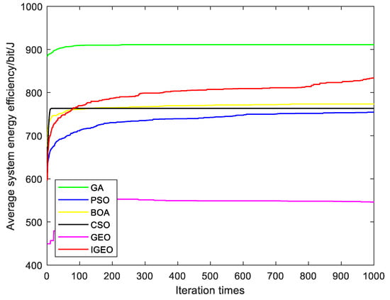
Figure 8.
Maximize the system benefit of the algorithms.
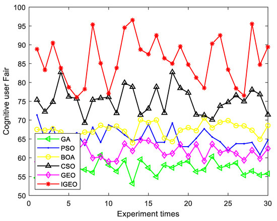
Figure 9.
Fairness under different parameter environments.
To investigate the impact of different numbers of users on the average system benefit, in this study, the number of available channels is maintained at a constant M = 10 in the environment, while increasing the number of SUs N from 10 to 30, with an increment of 2. The relationship between the number of users and the average benefit is analyzed, as shown in Figure 10. The results indicate that the average benefit of the cognitive radio system gradually decreases with increasing numbers of SUs. However, the IGEO algorithm outperforms the GA, PSO, BOA, CSA, and GEO algorithms in terms of the average system benefit value obtained.
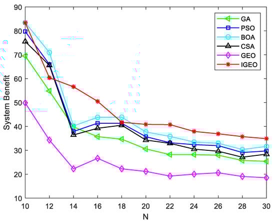
Figure 10.
The association between average benefit and user count.
On the other hand, this study looks into how different channel counts affect the overall value of the system. The average advantage of the system for different numbers of channels is obtained while increasing M from 10 to 30, with an increment of 2, as shown in Figure 11. Our results show that when the number of possible spectra in the region rises, the average benefit of the channel gradually increases. Notably, with the exception of BOA, the average benefit of the IGEO algorithm is higher than that of other methods. This underlines once more how well the improved algorithm allocates spectrum.
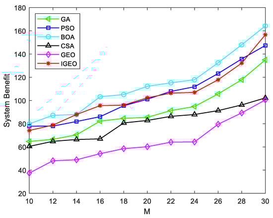
Figure 11.
The association between average benefit and frequency spectrum count.
4.3. Engineering Applications
To further validate the performance and practical effectiveness of the improved algorithm, in this article, five classic engineering problems were selected, and comparative experiments were conducted with other algorithms. All five engineering problems are static single-objective constrained optimization problems, which can be generally expressed as follows:
where represents the objective function, and and represent the constraint conditions.
To more effectively handle the constraint conditions, in this article, penalty functions are employed, which can be expressed as:
where represents the final objective function, and and represent the penalty coefficients. All algorithms are independently tested 30 times.
4.3.1. Piston Rod Design Problem
A rarely encountered static, single-objective constrained problem is the piston rod optimization problem. By maximizing the locations of the piston components H, B, D, and X as the piston rod advances from 0 degrees to 45 degrees, as indicated in Appendix A, its primary goal is to reduce fuel consumption. The basic model is expressed in Appendix B.
In the piston rod design problem, the IGEO algorithm is compared with GWO, PSO, SCA, SSA, WOA, GEO, and GEO_DLS. The minimum cost and corresponding optimal variable values obtained by the above algorithms can be found in Table 14. Among the algorithms, IGEO achieves the best performance in the piston rod design problem, with the lowest cost of 0.0003717.
Table 14.
Comparison of the best results and the statistical results obtained using different optimizers for the piston rod design problem.
4.3.2. I Beam Design Problem
The goal in the I beam structural design problem is to minimize vertical deflection by optimizing the length, height, and two thicknesses. Appendix A contains a structural schematic diagram, which depicts the left and major views of the I beam. For ease of computation, let . The mathematical model is expressed in Appendix B.
The performance of IGEO when designing I beams is compared to that of other algorithms, including GWO, PSO, SCA, SSA, WOA, GEO, and GEO_DLS. The comparison results are presented in Table 15, where it can be observed that both GEO and GEO_DLS yield an optimal value of 0.001644. However, the key difference lies in the very small standard deviation of IGEO, indicating its high stability in solving the problem.
Table 15.
Comparison of best results and the statistical results obtained using different optimizers for I beam design problem.
4.3.3. Car Side Impact Design Problem
The car side impact design problem is a static constrained optimization problem with a single objective and multiple variables. Its main objective is to minimize the total weight of the vehicle. The mathematical model is presented in Appendix B, and the meanings of the specific parameters can be found in [57].
The performances of different algorithms when designing car side collisions are compared in Table 16. Among the compared algorithms, which included GWO, PSO, SCA, SSA, WOA, GEO, and GEO_DLS, IGEO achieved the best result, with the minimum value of 21.8829.
Table 16.
Comparison of the best results and the statistical results obtained using different optimizers for the car side impact design problem.
4.3.4. Cantilever Beam Design Problem
The cantilever beam optimization problem involves five variables and a vertical displacement constraint, where each variable has a constant thickness, and the objective is to minimize the weight of the beam. A schematic diagram for this problem is presented in Appendix A. The mathematical model for this problem is given in Appendix B.
After applying various optimization algorithms such as GWO, PSO, SCA, SSA, WOA, GEO, and GEO_DLS, IGEO was used to optimize the cantilever beam design problem. The results obtained using these algorithms are presented in Table 17, where it can be observed that IGEO achieved the best result, with a value of 1.179635.
Table 17.
Comparison of the best results and the statistical results obtained using different optimizers for the cantilever beam design problem.
4.3.5. Three-Bar Truss Design Problem
In the classic three-bar truss engineering design problem, the aim is to minimize the weight of a symmetrical light bar structure that is subject to constraints on stress, deflection, and buckling. The mathematical model for this problem is presented in Appendix B, and the structural diagram can be found in Appendix A.
Table 18 presents the results of various optimization algorithms, including GWO, PSO, SCA, SSA, WOA, GEO, and GEO_DLS, as well as the comparison algorithm GEO_DLS, and IGEO for the three-bar truss design problem. The table indicates that IGEO achieved the best results, with a minimum value of 259.8111.
Table 18.
Comparison of the best results and the statistical results obtained using different optimizers for the three-bar truss design problem.
5. Conclusions
The principle and position update formula of the original golden eagle optimization method were explored, and a hybrid golden eagle optimization algorithm (IGEO) based on Arnold mapping and nonlinear convex decreasing weight was proposed. Using 12 benchmark functions, CEC2021, and the Wilcoxon, Friedman, and Holm tests, it was confirmed that the proposed IGEO has better search performance and stronger resilience. Additionally, the impact of the single-strategy method on the algorithm was also studied. After conducting simulation tests, the enhanced IGEO was applied to the model of the traditional cognitive radio spectrum allocation problem. It was discovered that IGEO had the best overall performance, and was able to allocate the spectrum well when compared to GA, PSO, and other methods. To test the proposed IGEO’s problem-solving abilities, five real-world technical design problems were also addressed, and the solutions were contrasted with other methods. The IGEO methodology is supported by all of the findings, feedback, and analyses as being a superior approach that can be used to tackle challenging engineering optimization problems. In future research, IGEO is expected to be applied to more practical spectrum allocation problems in order to investigate the algorithm’s additional capabilities.
Author Contributions
Conceptualization, J.D.; methodology, J.D.; software, J.D.; validation, J.D., D.Z. and Q.H.; formal analysis, J.D.; writing—original draft preparation, J.D.; writing—review and editing, J.D. and L.L.; resources, D.Z. and Q.H.; All authors have read and agreed to the published version of the manuscript.
Funding
This research and the APC were funded by National Natural Science Foundation of China, grant number No 62062021, 61872034, 62166006; Natural Science Foundation of Guizhou Province, grant number [2020]1Y254; Guizhou Provincial Science and Technology Projects, grant number Guizhou Science Foundation-ZK [2021] General 335.
Institutional Review Board Statement
Not applicable.
Informed Consent Statement
Not applicable.
Data Availability Statement
The study did not report any data.
Acknowledgments
The author is extremely thankful to anonymous referees and the editor for their valuable comments towards improving the manuscript.
Conflicts of Interest
The authors declare no conflict of interest.
Appendix A
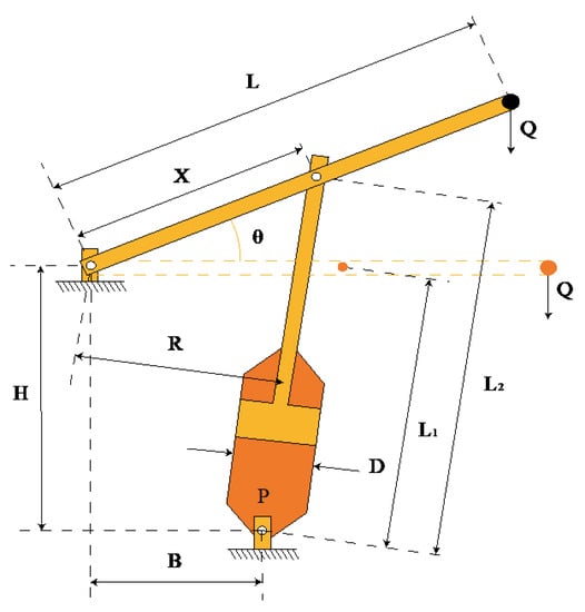
Figure A1.
Piston rod structure.
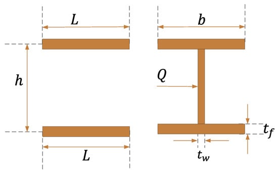
Figure A2.
I beam structure.
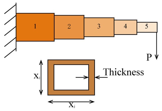
Figure A3.
Cantilever beam structure.
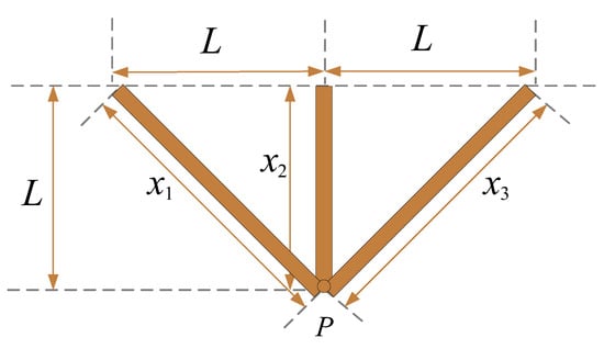
Figure A4.
Three-bar truss structure.
Appendix B
Appendix B.1. Piston Rod Design Problem
Minimize
Subject to
where .
Appendix B.2. I Beam Design Problem
Minimize
Subject to
where
Appendix B.3. Cantilever Beam Design Problem
Minimize
Subject to
where
Appendix B.4. Car Side Impact Design Problem
Minimize
Subject to
where
Appendix B.5. Three Bar Truss Design Problem
Minimize
Subject to
where
References
- Zervoudakis, K.; Tsafarakis, S. A mayfly optimization algorithm. Comput. Ind. Eng. 2020, 145, 106559. [Google Scholar] [CrossRef]
- Nematollahi, F.A.; Rahiminejad, A.; Vahidi, B. A novel physical based meta-heuristic optimization method known as Lightning Attachment Procedure Optimization. Appl. Soft Comput. 2017, 59, 596–621. [Google Scholar] [CrossRef]
- Haider, W.B.; Ur, N.R.; Asma, N.; Nisar, K.; Ibrahim, A.; Shakir, R.; Rawat, D.B. Constructing Domain Ontology for Alzheimer Disease Using Deep Learning Based Approach. Electronics 2022, 11, 1890. [Google Scholar]
- Ji, Z.; Chang, J.; Guo, X.; Wang, J.; Yang, H.; Wang, L.; Jiang, H. Ultrawide coverage receiver based on compound eye structure for free space optical communication. Opt. Commun. 2023, 545, 129740. [Google Scholar] [CrossRef]
- Zhu, C.; Ji, Q.; Guo, X.; Zhang, J. Mmwave massive MIMO: One joint beam selection combining cuckoo search and ant colony optimization. EURASIP J. Wirel. Commun. Netw. 2023, 2023, 65. [Google Scholar] [CrossRef]
- Yang, X.-S.; Deb, S. Engineering optimisation by cuckoo search. Int. J. Math. Model. Numer. Optim. 2010, 1, 330–343. [Google Scholar] [CrossRef]
- Majid, M.; Goel, L.; Saxena, A.; Srivastava, A.K.; Singh, G.K.; Verma, R.; Bhutto, J.K.; Hussein, H.S. Firefly Algorithm and Neural Network Employment for Dilution Analysis of Super Duplex Stainless Steel Clads over AISI 1020 Steel Using Gas Tungsten Arc Process. Coatings 2023, 13, 841. [Google Scholar] [CrossRef]
- Dervis, K.; Bahriye, B. A powerful and efficient algorithm for numerical function optimization: Artificial bee colony (ABC) algorithm. J. Glob. Optim. 2007, 39, 459–471. [Google Scholar]
- Seyedali, M.; Andrew, L. The Whale Optimization Algorithm. Adv. Eng. Softw. 2016, 95, 51–67. [Google Scholar]
- Mirjalili, S.; Mirjalili, S.M.; Lewis, A. Grey Wolf Optimizer. Adv. Eng. Softw. 2014, 69, 46–61. [Google Scholar] [CrossRef]
- Gaurav, D.; Vijay, K. Seagull optimization algorithm: Theory and its applications for large-scale industrial engineering problems. Knowl. Based Syst. 2018, 165, 169–196. [Google Scholar]
- Mirjalili, S.; Gandomi, A.H.; Mirjalili, S.Z.; Saremi, S.; Faris, H.; Mirjalili, S.M. Salp Swarm Algorithm: A bio-inspired optimizer for engineering design problems. Adv. Eng. Softw. 2017, 114, 163–191. [Google Scholar] [CrossRef]
- Arora, S.; Singh, S. Butterfly optimization algorithm: A novel approach for global optimization. Soft Comput. 2019, 23, 715–734. [Google Scholar] [CrossRef]
- Hassan, N.; Bangyal, W.H.; Khan, S.M.A.; Nisar, K.; Ibrahim, A.A.A.; Rawat, D.B. Improved Opposition-Based Particle Swarm Optimization Algorithm for Global Optimization. Symmetry 2021, 13, 2280. [Google Scholar] [CrossRef]
- Yang, L.; He, Q.; Yang, L.; Luo, S. A Fusion Multi-Strategy Marine Predator Algorithm for Mobile Robot Path Planning. Appl. Sci. 2022, 12, 9170. [Google Scholar] [CrossRef]
- Li, S.; He, Q. Improved Feature Selection for Marine Predator Algorithm. Comput. Eng. Appl. 2023, 59, 168–179. [Google Scholar]
- Xu, M.; Long, W.; Yang, Y. Planar-mirror reflection imaging learning based marine predators algorithm and feature selection. Comput. Appl. Res. 2023, 40, 394–398 + 444. [Google Scholar]
- Ma, C.; Zeng, G.; Huang, B.; Liu, J. Marine Predator Algorithm Based on Chaotic Opposition Learning and Group Learning. Comput. Eng. Appl. 2022, 58, 271–283. [Google Scholar]
- Xu, H.; Zhang, D.; Wang, Y.; Song, T.T. Application of Improved Whale Algorithm in Cognitive Radio Spectrum Allocation. Comput. Simul. 2021, 38, 431–436. [Google Scholar]
- Xu, H.; Zhang, D.; Wang, Y.; Song, T.T. Spectrum allocation based on improved binary grey wolf optimizer. Comput. Eng. Des. 2021, 42, 1353–1359. [Google Scholar]
- Yin, D.; Zhang, D.; Zhang, L.; Cai, P.; Qin, W. Spectrum Allocation Strategy Based on Sparrow Algorithm in Cognitive Industrial Internet of Things. Data Acquis. Process. 2022, 37, 371–382. [Google Scholar]
- Zhang, D.; Wang, Y.; Zou, C.; Zhao, P.; Zhang, L. Resource allocation strategies for improved mayfly algorithm in cognitive heterogeneous cellular network. J. Commun. 2022, 43, 156–167. [Google Scholar]
- Meng, K.O.; Pauline, O.; Kiong, C.S. A new flower pollination algorithm with improved convergence and its application to engineering optimization. Decis. Anal. J. 2022, 5, 100144. [Google Scholar]
- Yang, X.; Wang, R.; Zhao, D.; Yu, F.; Huang, C.; Heidari, A.A.; Chen, H. An adaptive quadratic interpolation and rounding mechanism sine cosine algorithm with application to constrained engineering optimization problems. Expert Syst. Appl. 2023, 213, 119041. [Google Scholar] [CrossRef]
- Sabry, A.E.; Muhammed, M.H.; Khalaf, W.A. Letter: Application of optimization algorithms to engineering design problems and discrepancies in mathematical formulas. Appl. Soft Comput. J. 2023, 140, 110252. [Google Scholar]
- Mohammadi-Balani, A.; Nayeri, M.D.; Azar, A.; Taghizadeh-Yazdi, M. Golden eagle optimizer: A nature-inspired metaheuristic algorithm. Comput. Ind. Eng. 2021, 152, 107050. [Google Scholar] [CrossRef]
- Aijaz, M.; Hussain, I.; Lone, S.A. Golden Eagle Optimized Control for a Dual Stage Photovoltaic Residential System with Electric Vehicle Charging Capability. Energy Sources Part A Recovery Util. Environ. Eff. 2022, 44, 4525–4545. [Google Scholar] [CrossRef]
- Magesh, T.; Devi, G.; Lakshmanan, T. Improving the performance of grid connected wind generator with a PI control scheme based on the metaheuristic golden eagle optimization algorithm. Electr. Power Syst. Res. 2023, 214, 108944. [Google Scholar] [CrossRef]
- Kumar, A.G.D.; Vengadachalam, N.; Madhavi, S.V. A Novel Optimized Golden Eagle Based Self-Evolving Intelligent Fuzzy Controller to Enhance Power System Performance. In Proceedings of the 2022 IEEE 2nd International Conference on Sustainable Energy and Future Electric Transportation (SeFeT), Hyderabad, India, 4–6 August 2022; pp. 1–6. [Google Scholar]
- Sun, H. An extreme learning machine model optimized based on improved golden eagle algorithm for wind power forecasting. In Proceedings of the 2022 37th Youth Academic Annual Conference of Chinese Association of Automation (YAC), Beijing, China, 19–20 November 2022; pp. 86–91. [Google Scholar]
- Boriratrit, S.; Chatthaworn, R. Golden Eagle Extreme Learning Machine for Hourly Solar Irradiance Forecasting. In Proceedings of the International Conference on Electrical, Computer, Communications and Mechatronics Engineering (ICECCME), Maldives, Maldives, 16–18 November 2022; p. 9988106. [Google Scholar]
- Bandahalli Mallappa, P.K.; Velasco Quesada, G.; Martínez García, H. Energy Management of Grid Connected Hybrid Solar/Wind/Battery System using Golden Eagle Optimization with Incremental Conductance. Renew. Energy Power Qual. J. 2022, 20, 342–347. [Google Scholar] [CrossRef]
- Zhang, Z.-K.; Li, P.-Q.; Zeng, J.-J. Capacity Optimization of Hybrid Energy Storage System Based on Improved Golden Eagle Optimization. J. Netw. Intell. 2022, 7, 943–959. [Google Scholar]
- Boriratrit, S.; Fuangfoo, P.; Srithapon, C.; Chatthaworn, R. Adaptive meta-learning extreme learning machine with golden eagle optimization and logistic map for forecasting the incomplete data of solar irradiance. Energy AI 2023, 13, 100243. [Google Scholar] [CrossRef]
- Guo, J.-F.; Zhang, Y.-Q.; Xu, S.-B.; Lin, J.-Y. A Power System Profitable Load Dispatch Based on Golden Eagle Optimizer. J. Comput. 2022, 33, 145–158. [Google Scholar]
- Al-Gburi, Z.D.S.; Kurnaz, S. Optical disk segmentation in human retina images with golden eagle optimizer. Optik 2022, 271, 170103. [Google Scholar] [CrossRef]
- Dwivedi, A.; Rai, V.; Amrita; Joshi, S.; Kumar, R.; Pippal, S.K. Peripheral blood cell classification using modified local-information weighted fuzzy C-means clustering-based golden eagle optimization model. Soft Comput. 2022, 26, 13829–13841. [Google Scholar] [CrossRef]
- Justus, J.J.; Anuradha, M. A golden eagle optimized hybrid multilayer perceptron convolutional neural network architecture-based three-stage mechanism for multiuser cognitive radio network. Int. J. Commun. Syst. 2021, 35, 5054. [Google Scholar] [CrossRef]
- Eluri, R.K.; Devarakonda, N. Binary Golden Eagle Optimizer with Time-Varying Flight Length for feature selection. Knowl.-Based Syst. 2022, 247, 108771. [Google Scholar] [CrossRef]
- Zarkandi, S. Dynamic modeling and power optimization of a 4RPSP+PS parallel flight simulator machine. Robotica 2021, 40, 646–671. [Google Scholar] [CrossRef]
- Lv, J.X.; Yan, L.J.; Chu, S.C.; Cai, Z.M.; Pan, J.S.; He, X.K. A new hybrid algorithm based on golden eagle optimizer and grey wolf optimizer for 3D path planning of multiple UAVs in power inspection. Neural Comput. Appl. 2022, 34, 11911–11936. [Google Scholar] [CrossRef]
- Pan, J.-S.; Lv, J.-X.; Yan, L.-J.; Weng, S.-W.; Chu, S.-C.; Xue, J.-K. Golden eagle optimizer with double learning strategies for 3D path planning of UAV in power inspection. Math. Comput. Simul. 2022, 193, 509–532. [Google Scholar] [CrossRef]
- Ilango, R.; Rajesh, P.; Shajin Francis, H. S2NA-GEO method–based charging strategy of electric vehicles to mitigate the volatility of renewable energy sources. Int. Trans. Electr. Energy Syst. 2021, 31, 13125. [Google Scholar] [CrossRef]
- Jagadish Kumar, N.; Balasubramanian, C. Hybrid Gradient Descent Golden Eagle Optimization (HGDGEO) Algorithm-Based Efficient Heterogeneous Resource Scheduling for Big Data Processing on Clouds. Wirel. Pers. Commun. 2023, 129, 1175–1195. [Google Scholar] [CrossRef]
- Ghasemi, A.; Sousa, E.S. Spectrum sensing in cognitive radio networks: Requirements, challenges and design trade-offs. IEEE Commun. Mag. 2008, 46, 32–39. [Google Scholar] [CrossRef]
- Peng, C.; Zheng, H.; Zhao, B.Y. Utilization and fairness in spectrum assignment for opportunism tic spectrum access. Mob. Netw. Appl. 2006, 11, 555–576. [Google Scholar] [CrossRef]
- Wang, W.; Liu, X. List-coloring based channel allocation for open spectrum wireless networks. In Proceedings of the IEEE Vehicular Technology Conference, Stockholm, Sweden, 30 May–1 June 2005; pp. 690–694. [Google Scholar]
- Gandhi, S.; Buragohain, C.; Cao, L.; Zheng, H.; Suri, S. Towards real time dynamic spectrum auctions. Comput. Netw. 2009, 52, 879–897. [Google Scholar] [CrossRef]
- Ji, Z.; Liu, K.J.R. Dynamic spectrum sharing: A game theoretical overview. IEEE Commun. Mag. 2007, 45, 88–94. [Google Scholar] [CrossRef]
- Liu, Q.; Wang, C.; Li, X.; Gao, L. An improved genetic algorithm with modified critical path-based searching for integrated process planning and scheduling problem considering automated guided vehicle transportation task. J. Manuf. Syst. 2023, 70, 127–136. [Google Scholar] [CrossRef]
- Ahmed, A.M.; Rashid, T.A.; Saeed, S.A.M. Cat Swarm Optimization Algorithm: A Survey and Performance Evaluation. Comput. Intell. Neurosci. 2020, 2020, 4854895. [Google Scholar] [CrossRef]
- Mirjalili, S. SCA: A Sine Cosine Algorithm for solving optimization problems. Knowl.-Based Syst. 2016, 96, 120–133. [Google Scholar] [CrossRef]
- Nabil, E. A Modified Flower Pollination Algorithm for Global Optimization. Expert Syst. Appl. 2016, 57, 192–203. [Google Scholar] [CrossRef]
- Dong, H.B.; Li, D.J.; Zhang, X.P. Particle Swarm Optimization Algorithm with Dynamically Adjusting Inertia Weight. Comput. Sci. 2018, 45, 98–102, 139. [Google Scholar]
- Caraffini, F.; Iacca, G.; Neri, F.; Picinali, L.; Mininno, E. A CMA-ES Super-fit Scheme for the Re-sampled Inheritance Search. In Proceedings of the 2013 IEEE Congress on Evolutionary Computation, Cancun, Mexico, 20–23 June 2013; pp. 1123–1130. [Google Scholar]
- Tanabe, R.; Fukunaga, A.S. Improving the Search Performance of SHADE Using Linear Population Size Reduction. In Proceedings of the 2014 IEEE Congress on Evolutionary Computation (CEC), Beijing, China, 6–11 July 2014; pp. 1658–1665. [Google Scholar]
- Kumar, S.A. Multi-population-based adaptive sine cosine algorithm with modified mutualism strategy for global optimization. Knowl. Based Syst. 2022, 251, 109326. [Google Scholar]
Disclaimer/Publisher’s Note: The statements, opinions and data contained in all publications are solely those of the individual author(s) and contributor(s) and not of MDPI and/or the editor(s). MDPI and/or the editor(s) disclaim responsibility for any injury to people or property resulting from any ideas, methods, instructions or products referred to in the content. |
© 2023 by the authors. Licensee MDPI, Basel, Switzerland. This article is an open access article distributed under the terms and conditions of the Creative Commons Attribution (CC BY) license (https://creativecommons.org/licenses/by/4.0/).