Article

Parameter Optimization for Low-Rank Matrix Recovery in Hyperspectral Imaging

by
Monika Wolfmayr
1,2
1
Institute of Information Technology, Jamk University of Applied Sciences, 40101 Jyväskylä, Finland
2
Faculty of Information Technology, University of Jyväskylä, 40014 Jyväskylä, Finland
Appl. Sci. 2023, 13(16), 9373; https://doi.org/10.3390/app13169373
Submission received: 14 May 2023 / Revised: 4 August 2023 / Accepted: 16 August 2023 / Published: 18 August 2023

Abstract

:
An approach to parameter optimization for the low-rank matrix recovery method in hyperspectral imaging is discussed. We formulate an optimization problem with respect to the initial parameters of the low-rank matrix recovery method. The performance for different parameter settings is compared in terms of computational times and memory. The results are evaluated by computing the peak signal-to-noise ratio as a quantitative measure. The potential improvement in the performance of the noise reduction method is discussed when optimizing the choice of the initial values. The optimization method is tested on standard and openly available hyperspectral data sets, including Indian Pines, Pavia Centre, and Pavia University.

1. Introduction

In hyperspectral imaging (HSI), spectral signatures of objects are recorded for each image pixel. The spectral signature of an object is the reflectance variation or function with respect to the wavelength. It is important for characterizing materials and their properties. In HSI, different types of noise appear due to environmental or instrumental influences. The noises include Gaussian noise [1], impulse noise [2], dead pixels or lines [3], and stripes [4]. This has been recently discussed, for instance, in [5] and in the overview articles [6,7]. HSI combines spatial and spectral information in a hyperspectral data cube, as displayed in Figure 1. Naturally, the amount of generated data is huge, and an efficient and reliable approach to noise reduction takes advantage of the internal dependencies between the wavebands. HSI precision and reliability are essential for many applications, including digitalization and robotization in Earth and space exploration. The applications include agricultural monitoring [8], atmospheric science [9], geology [10], and space exploration [11]. Efficient and reliable noise reduction techniques are essential for image processing in practice regarding real-time decision-making and automation. In [12], various noise reduction techniques have been compared for hyperspectral image data in asteroid imaging, including also low-rank matrix recovery (LRMR).
LRMR is a low-rank modeling approach [13] and has been discussed among other advanced image processing methods in more detail in [6,7]. We use here LRMR together with the Go Decomposition (GoDec) numerical optimization algorithm as presented in [14] in the inner iteration steps of the approach for solving the restoration model. Parameter optimization in advanced image processing can provide important indirect information for control and real-time decision-making. The main idea here is to optimize the choice of the algorithm’s initial values in order to improve the performance of the noise reduction. We analyze the parameter choices, including applying nonlinear optimization methods as derived in [15]. The open, available hyperspectral data sets Indian Pines [16], Pavia Centre [17], and Pavia University [17] are used for the computational tests.
This work is part of the coADDVA—ADDing VAlue by Computing in Manufacturing project funded by the Regional Council of Central Finland/Council of Tampere Region and European Regional Development Fund. It supports the project’s goals to improve the efficiency of robotics by developing optimal control methods leading to flexible imaging and automation in image processing.
The article is organized as follows: In Section 2, the methods are discussed, including LRMR and the optimization applied to its initial parameter settings. The used data sets are presented. Section 3 presents the computational results. Section 4 discusses the results according to the existing literature and possible future work. Finally, Section 5 presents the main contributions of this work.

2. Methods and Materials

2.1. Methods

The first LRMR model was proposed in [18] as a robust principle component analysis approach. It was further developed in [13] for hyperspectral image restoration by combining nonlinear optimization in the inner iteration loop in order to solve the restoration model. In this work, we apply optimization with respect to the initial parameters in terms of an outer iteration loop.
In the following, we present the LRMR model. Given the real matrix D of size m × n containing the observed data and assuming corruption by the sparse error matrix S and random Gaussian noise modeled by the matrix N, the goal is to recover the low-rank matrix L with D = L + S + N , which are all real-number matrices of the same size: m × n . The minimization problem
min L , S D L S F 2 s . t . rank ( L ) r , card ( S ) p
is solved, with r denoting the upper bound for the rank of L and p for the cardinality of S, which is related to the estimation of noise corruption. The norm · F denotes the Frobenius-norm. The formulation (1) of LRMR can be found in [13,14]. Redundancies between the wavebands yield the low-rank property required for LRMR. LRMR modeling is then applied together with the GoDec algorithm [14] in order to solve the subproblems exploiting the low-rank property of HSI. The subproblems are created by taking subcubes centered at a pixel in the spatial dimension. Thus, if the whole data cube is of size m × n × w , where w denotes the number of spectral reflectance bands, then the subcubes are of size b × b × w , with b < m and b < n . We define the entries of the subcube’s spectral band by the spectral band. The entries of each subcube band–by-band are then organized in lexicographical order to obtain two-dimensional matrices of size b 2 × w . The subcubes are then processed iteratively, providing local image restoration. We denote further the iteration stepsize by s. More details on the specific LRMR model can be found in [13] and on GoDec in [14].
The main focus of this work is the detailed investigation of the LRMR method with respect to the starting values for its main variable parameters, including rank r and blocksize of the subcubes b, estimation parameter for the percentage of noise corruption p, and stepsize s of the inner iteration. In the following, we denote by r, p, b, and s the initial settings. We apply nonlinear optimization in order to determine the best parameter values for the parameter settings with respect to the peak signal-to-noise ratio (PSNR). We choose the Nelder–Mead simplex algorithm as presented in [15] for the nonlinear optimization. The PSNR is computed by
PSNR = 10 log 10 max ( C ) 2 m n w C C ˜ 2 ,
where C and C ˜ denote the original and denoised data cube, respectively. The sizes of the spatial and spectral dimensions are denoted by m , n , and w. The performance of LRMR is analyzed in terms of computational efficiency and memory with regard to different parameter choices. The computational time taken by the algorithm in MATLAB and Python is compared in order to study the performance of LRMR and differences in the implementation between the two programming languages. The goal is to investigate possible difficulties with parameter optimization.

2.2. Materials

We present the data sets used in this work.

2.2.1. Indian Pines Data Set

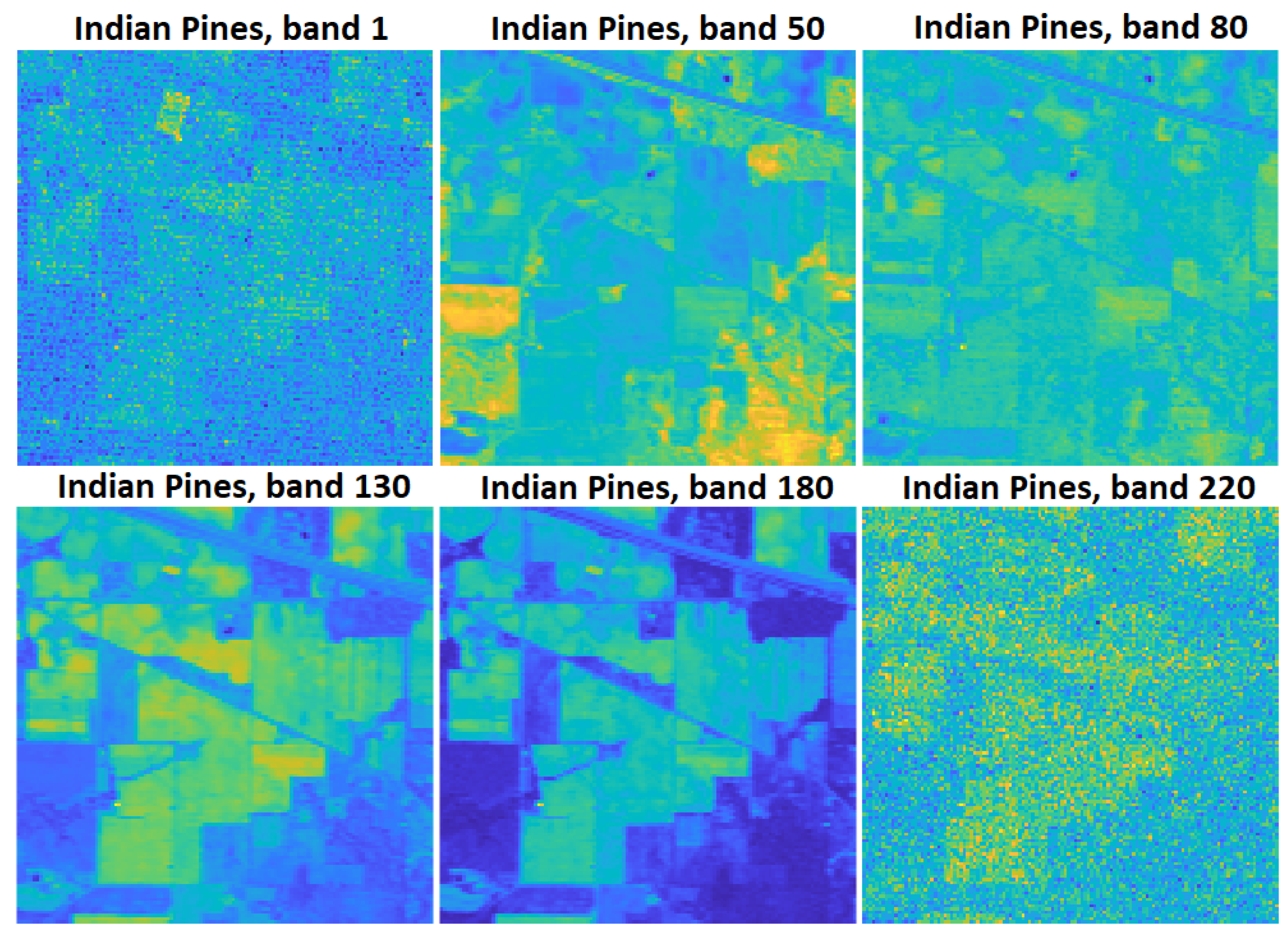
The Indian Pines data set covers the Indian Pines test site, which is located in northwestern Indiana. It shows mainly agriculture and forest. The data set consists of 224 spectral reflectance bands and is 145 × 145 pixels. The wavelength range lies between 0.4 and 2.5 × 10 6 m. The Indian Pines data set is openly available in [16].
Figure 2 shows the scene for six different spectral reflectance bands: 1, 50, 80, 130, 180, and 220. Different bands show different layers of materials’ spectral signatures.

2.2.2. Pavia Centre Data Set

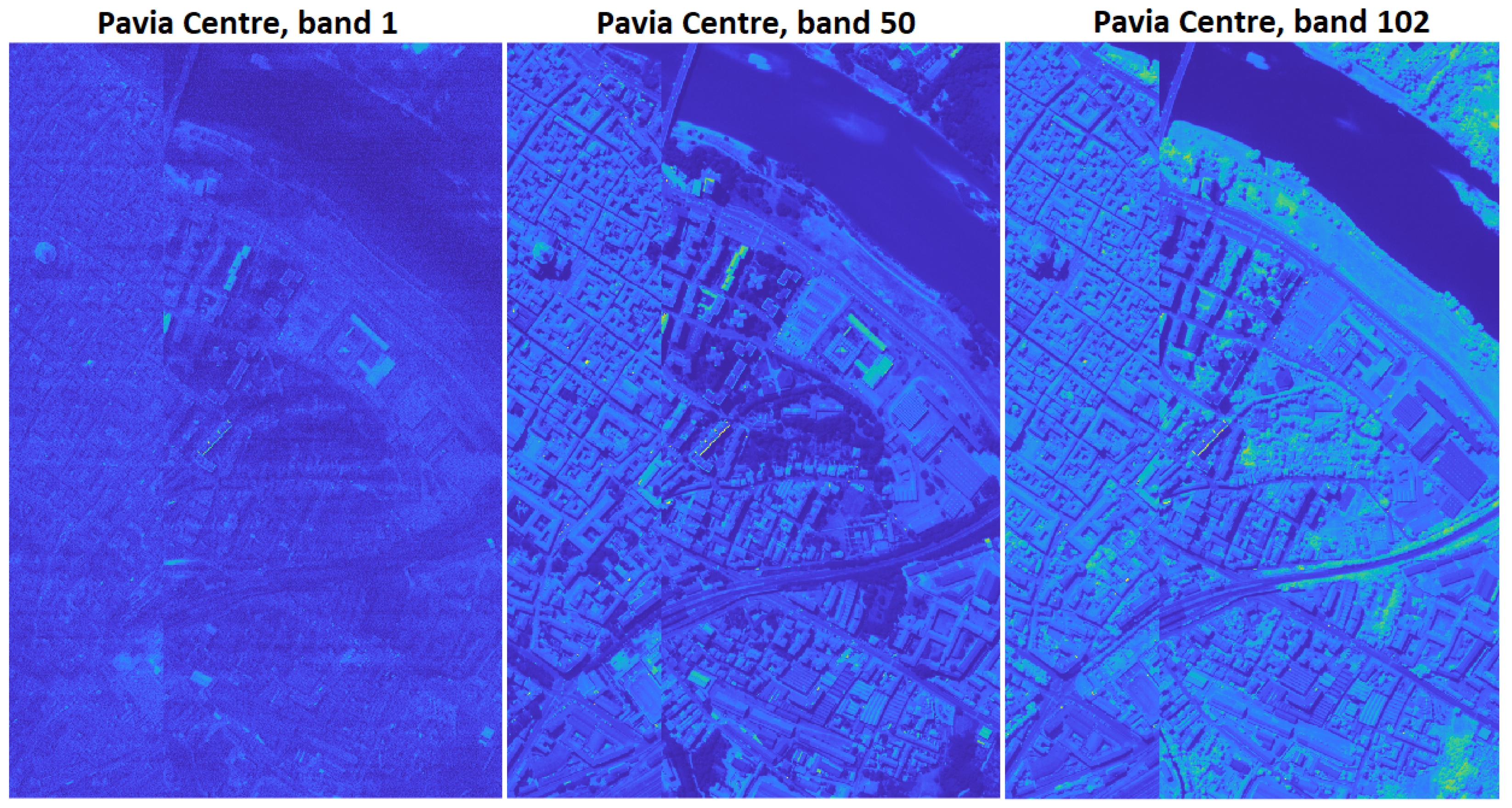
The data set contains scenes from the center of Pavia in northern Italy. It consists of 102 spectral reflectance bands and is 1096 × 1096 pixels. The set is openly available in [17].
Figure 3 shows the scene for three different spectral reflectance bands: 1, 50, and 102.

2.2.3. Pavia University Data Set

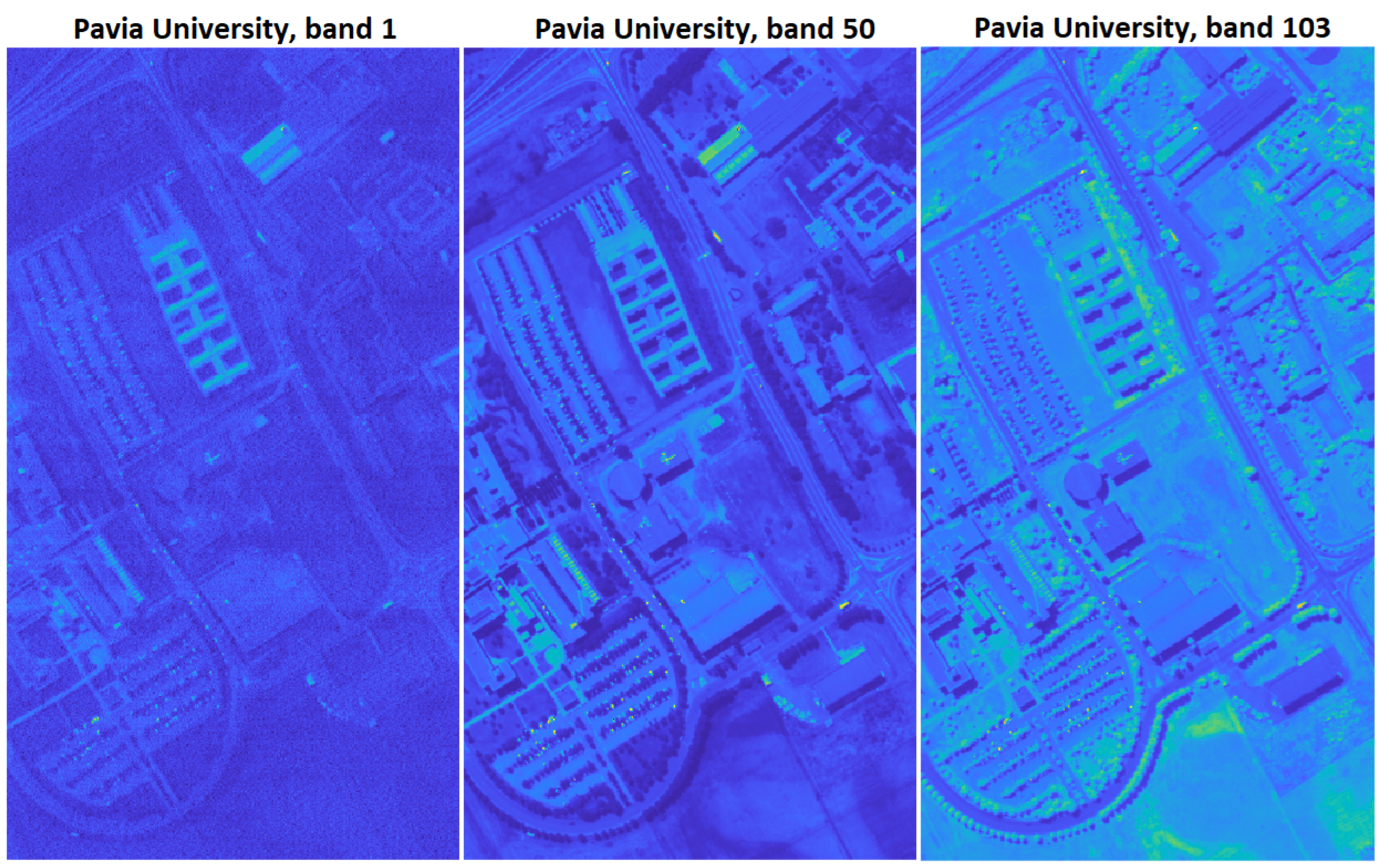
The data set contains scenes from the university in Pavia in northern Italy. It consists of 103 spectral reflectance bands and is 610 × 610 pixels. The set is openly available in [17].
Figure 4 shows the scene for three different spectral reflectance bands: 1, 50, and 103.

3. Results

We analyze how different parameter settings affect the PSNR and computational times. We are able to show that different parameter values and their combinations have an effect on the PSNRs and computational times of the LRMR method. The initial parameter values are optimized with respect to PSNR and CPU time. The parameter value combinations are studied in detail, and the results are presented visually.
We study the initial parameter value combinations for three integer-valued parameters—r, s, and b—and one real-valued parameter p. We apply nonlinear optimization with respect to the real-valued noise estimation parameter p, which results in an improvement in PSNR. The integer parameters are analyzed on a series of test sets. The optimized values are chosen according to their best PSNR performance. For all analyzed settings and resulting combinations, we show CPU times in MATLAB and Python. The computational experiments are performed on a laptop with an Intel(R) Core(TM) i5-8250U CPU @ 1.60 GHz 1.80 GHz processor and 16.0 GB RAM.
Figure 5 shows the performance of the method for a noise-corrupted waveband of the Indian Pines data set [16] for the parameter settings r = 7 , p = 0.15 , b = 20 , and s = 8 .

3.1. Parameter Analysis for r

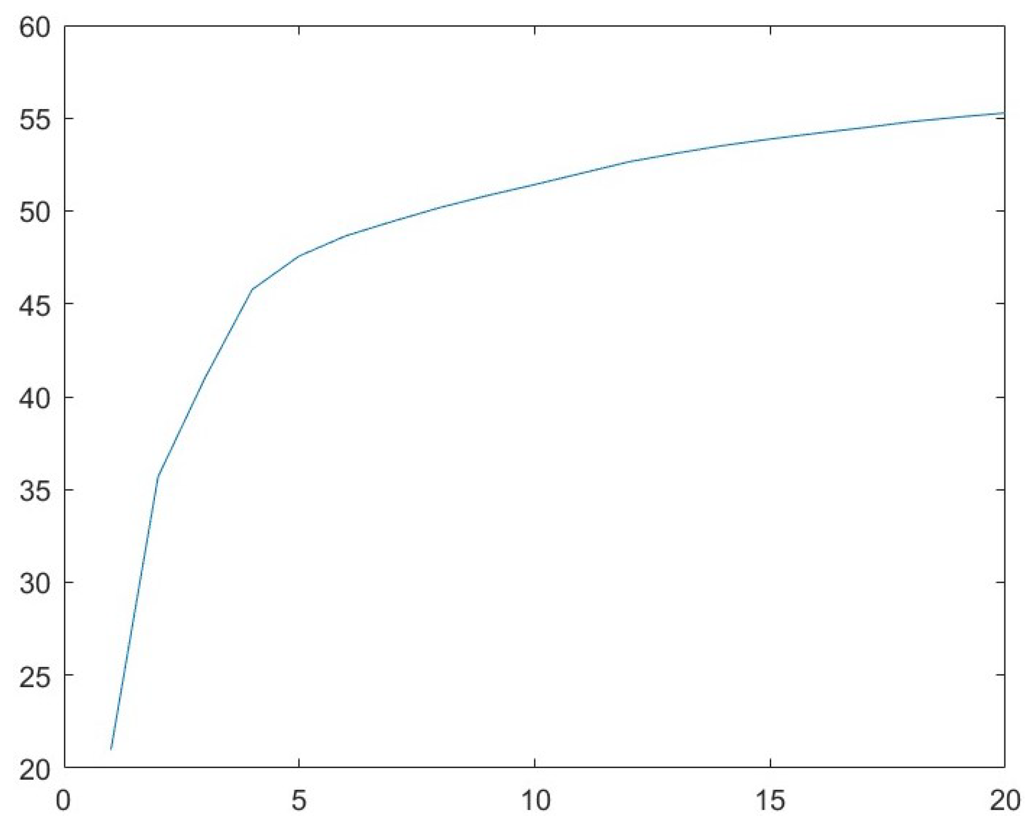
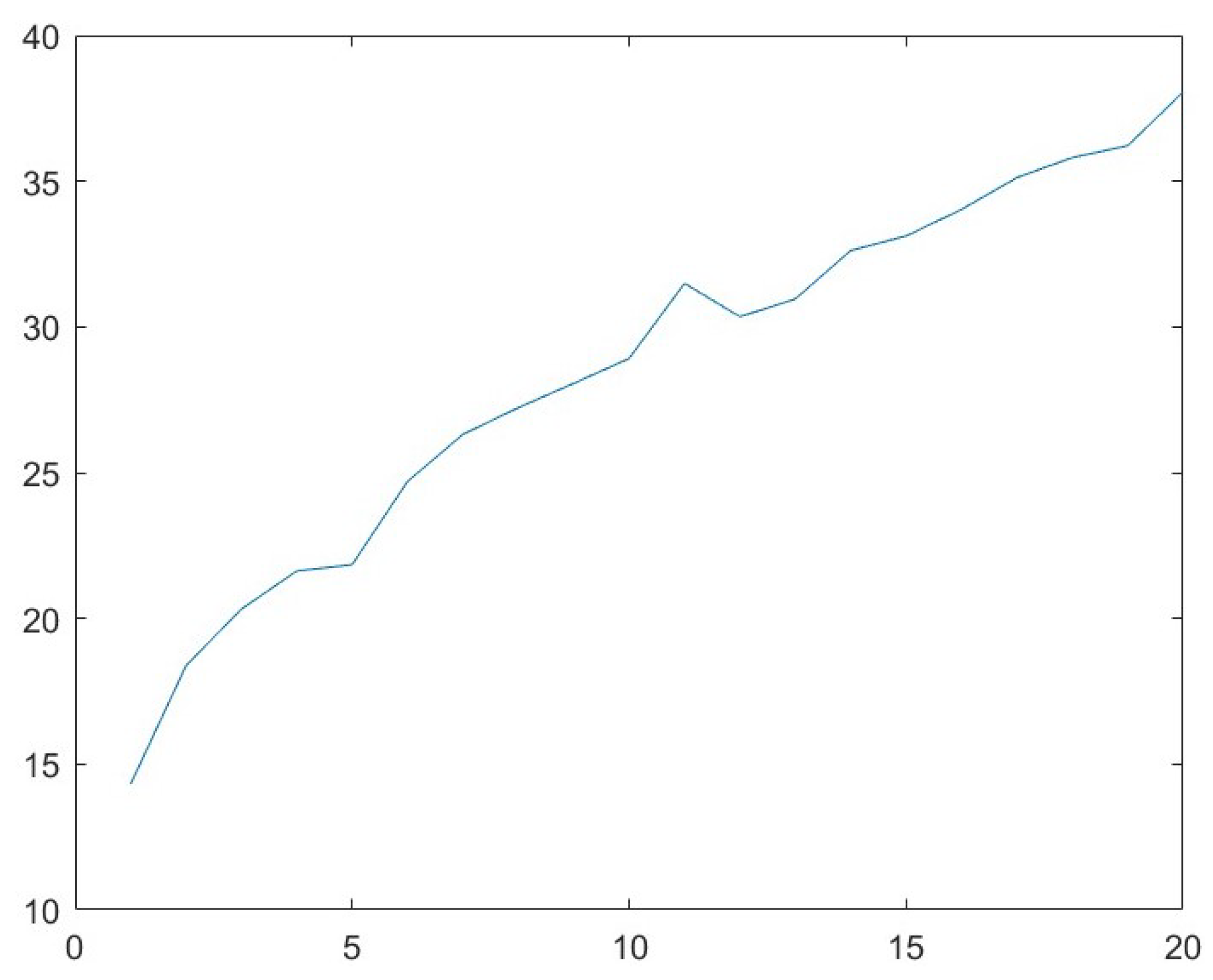
The rank parameter r describes the upper bound for the rank of the low-rank matrix describing the noise-free signal of the data cube. The value should be as small as possible while not underestimating the noise intensity of the image data. Small values provide shorter computational times, while larger values provide higher PSNR values. We vary the starting value for the rank parameter r between 1 and 20. The other parameters are kept at p = 0.15 , b = 20 , and s = 8 . Figure 6 shows the PSNR values for different values of r. In general, higher values of r provide larger PSNR values. The analysis shows that a value of r 4 is sufficient. The largest gradient step is already taken from r = 1 to r = 2 . The computational times in MATLAB are shown in Figure 7. A larger rank value r results in a larger computational time. The computational tests were computed on the Indian Pines data set.
In the following, we present the PSNR, the gradient of the PSNR denoted as ∇PSNR, and computational times in seconds in MATLAB and Python, denoted as t M a t l a b and t P y t h o n , respectively, in Table 1. Lower rank values are better in terms of computational effort.
The computational effort is significantly more efficient in MATLAB. The analysis for Indian Pines suggests choosing r = 5 . This parameter choice provides a sufficient balance between PSNR and computational time.

3.2. Parameter Analysis for s

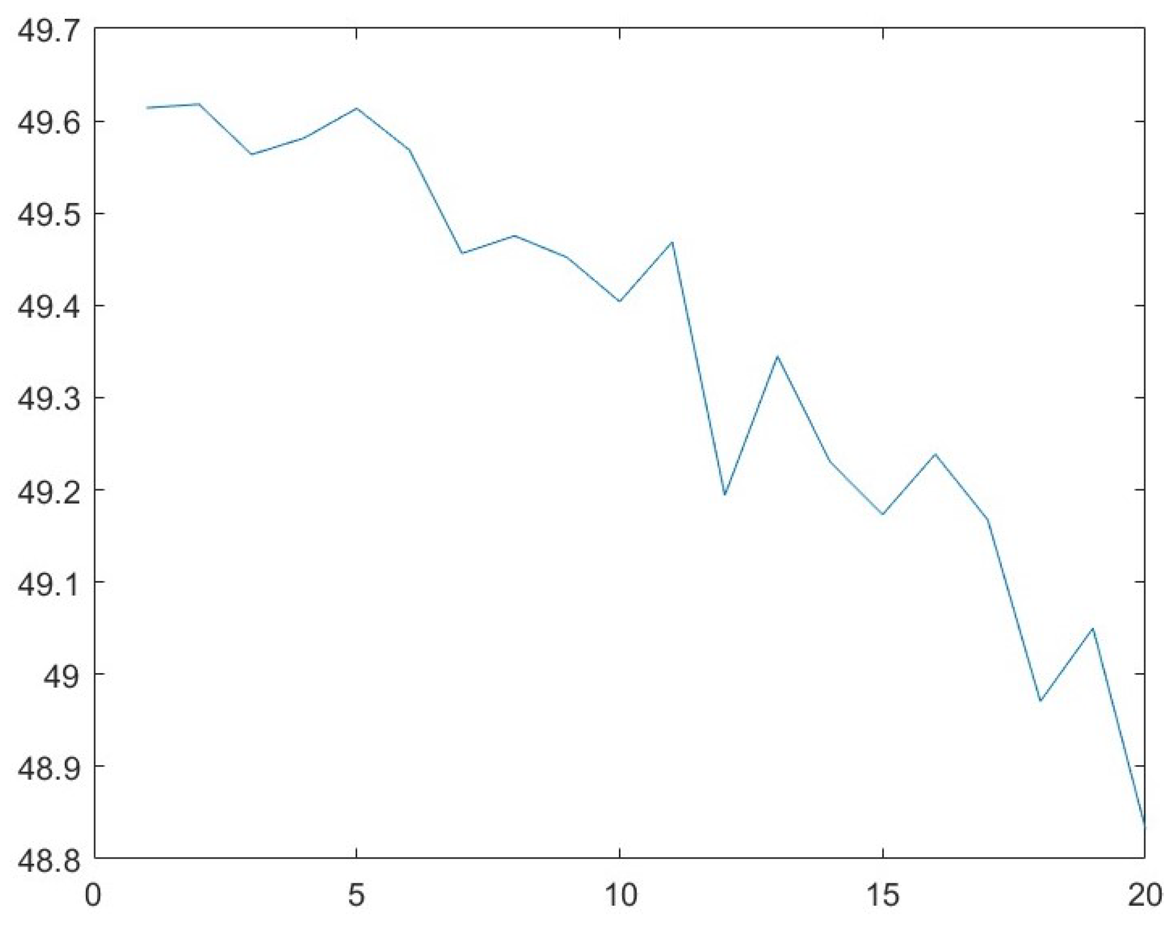
The parameter s describes the iteration stepsize for processing the subcubes of LRMR’s local image restoration. We vary the parameter value for the stepsize s between 1 and 20. The other parameter values are kept at r = 7 , p = 0.15 , and b = 20 . Figure 8 shows the PSNR values for different values of s. The trend shows that larger values for the stepsize s yield smaller PSNR values. Hence, smaller values for s are preferred, since we target a larger PSNR. The computational times in MATLAB are shown in Figure 9. The computational times are smaller for larger stepsizes s. However, the CPU times decrease significantly for stepsizes larger than 4. The computational tests were computed on the Indian Pines data set.
In the following, we present the computational times in seconds in MATLAB and Python in Table 2. Also, the gradient values for the computational times in MATLAB t M a t l a b are presented. The result is that a balance between smaller stepsizes that produce better PSNRs and larger stepsizes that are better in terms of computational time and effort has to be achieved. However, note that the difference in PSNR values is not significant, as Figure 8 shows. Figure 9 and the gradient values for the CPU times in Table 2 show clearly that a stepsize s 4 provides significant improvement regarding computational times.
As for the rank value r, the computational effort is significantly better in MATLAB than in Python.

3.3. Parameter Analysis for r and s

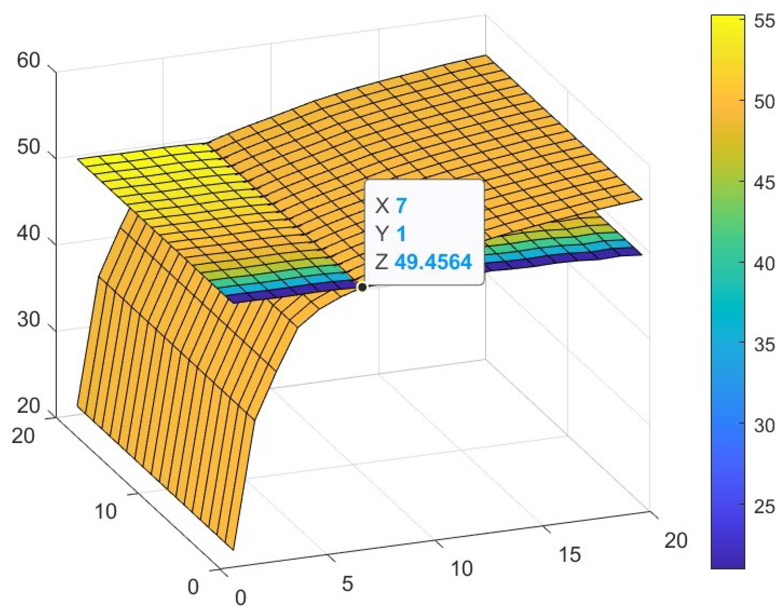
In this parameter analysis, we study how the parameter choices for r and s influence each other. Figure 10 shows the PSNRs for different rank r and stepsize s values, whereas the other parameter values b and p are set as b = 20 and p = 0.15 . The point of intersection is marked and corresponds to r = 7 and to values for s [ 1 , 20 ] . Again, r = 7 is shown to be the optimized parameter choice, whereas values for s show no significant difference in PSNRs. The tests were computed on the Indian Pines data set.

3.4. Parameter Analysis for b

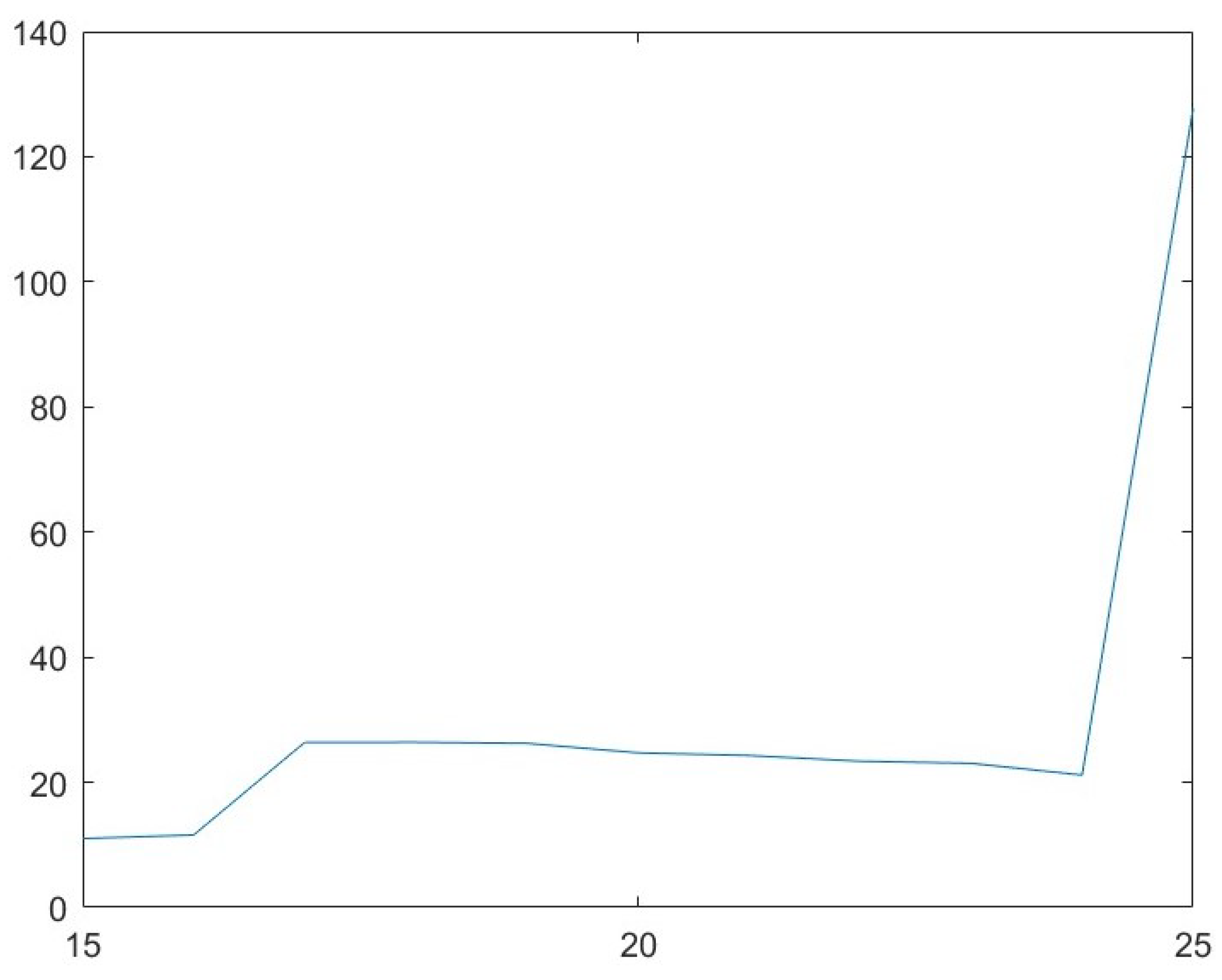
The blocksize of the subcubes for local restoration of LRMR is denoted by b. The parameter choice is significant, since naturally, the size of the subcubes provides accuracy and computational effort to the restoration. We vary the starting value for the blocksize parameter b between 15 and 25. Smaller values for b have not provided successful computations and errors in PSNR. The other parameters are kept as r = 7 , p = 0.15 , and s = 8 . Figure 11 shows the PSNR values for different values of b. The PSNR values are linearly decreasing with respect to increasing blocksize. Figure 12 shows the computational times in seconds in MATLAB. Apart from the large leap at the end and the smaller leap at the beginning, the computational time regarding the change in blocksize seems not to be affected significantly, although a weak trend towards increasing PSNR with increasing blocksize seems to be visible. We present the computational results for the Indian Pines data set.
In the following, we present the computational times in seconds in MATLAB and Python in Table 3.
Again, the computational effort is better in MATLAB R2022a.

3.5. Parameter Analysis for p

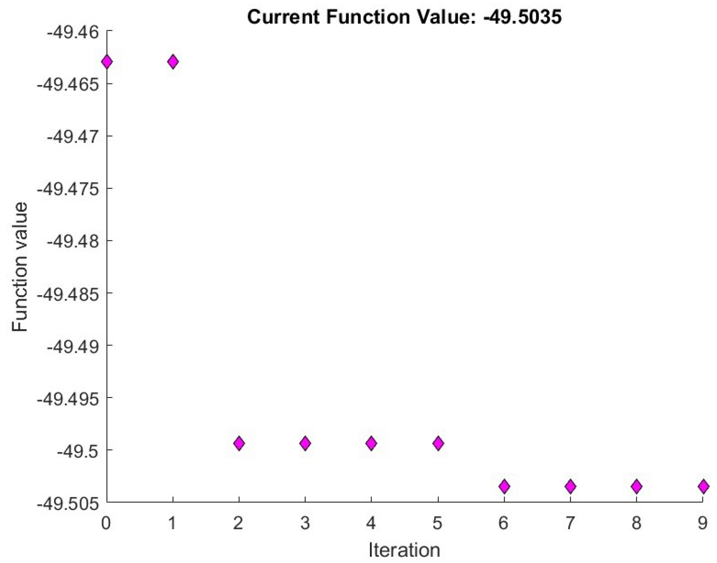
The parameter p describes an initial estimation of the amount of noise corruption in the data cube. It is the only real-valued parameter of LRMR’s initial parameters. Hence, nonlinear optimization can be applied to determine the optimal initial value for p. We present results for the nonlinear optimization method: the direct search method (i.e., the Nelder–Mead simplex algorithm [15]). We applied the method on the different test sets and varied the starting value for p. The other parameters were set as r = 7 , b = 20 , and s = 8 . We computed the optimization results of this section in MATLAB. In Figure 13, the negative PSNR values of the iteration steps of the nonlinear minimization method, the Nelder–Mead simplex algorithm, computed with respect to p are presented. We present the results for the Indian Pines data set. The starting value p = 0.15 was chosen.
The results in Figure 13 show convergence towards a local minimum. The value yields an improvement in PSNR. The computational tests show proper performance applying the Nelder–Mead simplex algorithm, including convergence and computational effort. However, the method is searching for a local optimum and, hence, has its limitations. The starting value is crucial. We include a table of final minimization function values and values for p for different starting values (Table 4). The stopping criteria were chosen as follows: the error in the function value is smaller than 10 15 , the error in the optimization parameter value is smaller than 10 9 , the maximum of function evaluations in one iteration step equals 20, and the overall maximum number of outer iteration steps equals 20.
We propose the choice of p = 0.15 for further computations on the data sets used in this work. It is numerically stable and provides sufficient PSNR values. Higher starting values than 1 e + 1 have not provided sufficient convergence.
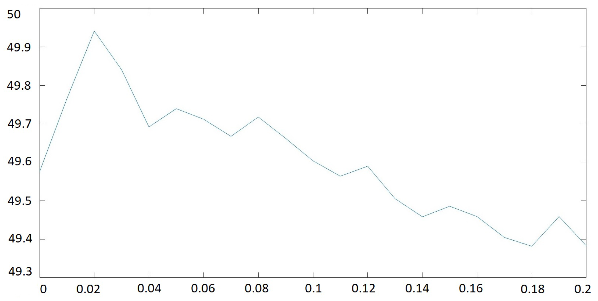
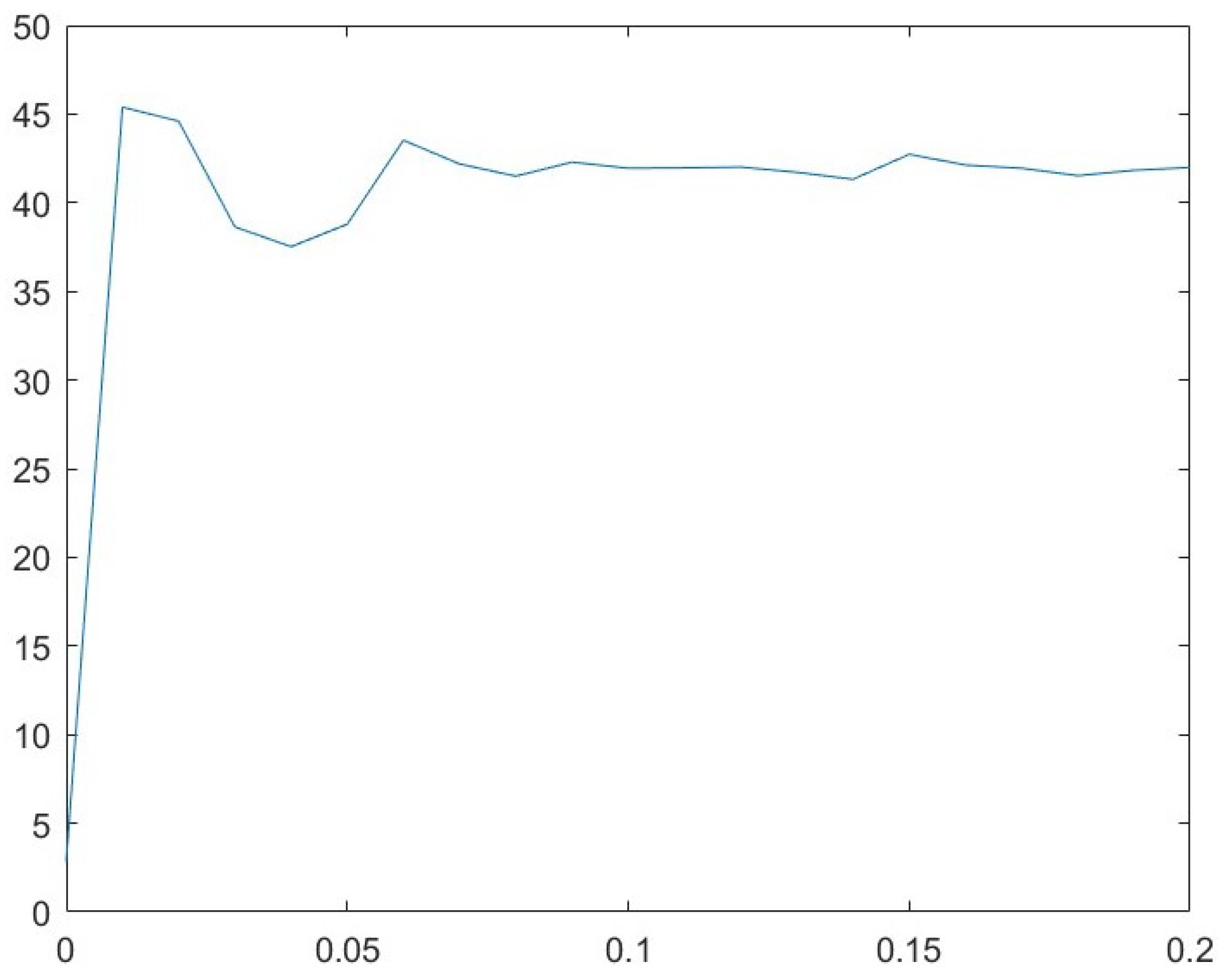
As a second test, we computed the PSNR and computational times for different values of p [ 0 , 0.2 ] to test different starting values. The Indian Pines test set was used again for a qualitative parameter analysis. Figure 14 shows the PSNR values for different p values. The figure suggests choosing a smaller starting value for p, which coincides with Table 4. Figure 15 shows the CPU times for different p values. The CPU times seem not to be significantly affected in this range of p.

3.6. Optimized Parameter Choice

Combining the results of the previous subsections, we present the resulting images for the optimized values. We propose the following settings: r = 7 , s = 8 , b = 20 , and p = 0.15 .

3.6.1. Indian Pines Data Set

The result of applying LRMR with the optimized parameter setting is shown in Figure 16.

3.6.2. Pavia Centre Data Set

The result of applying LRMR with the optimized parameter setting is shown in Figure 17.

3.6.3. Pavia University Data Set

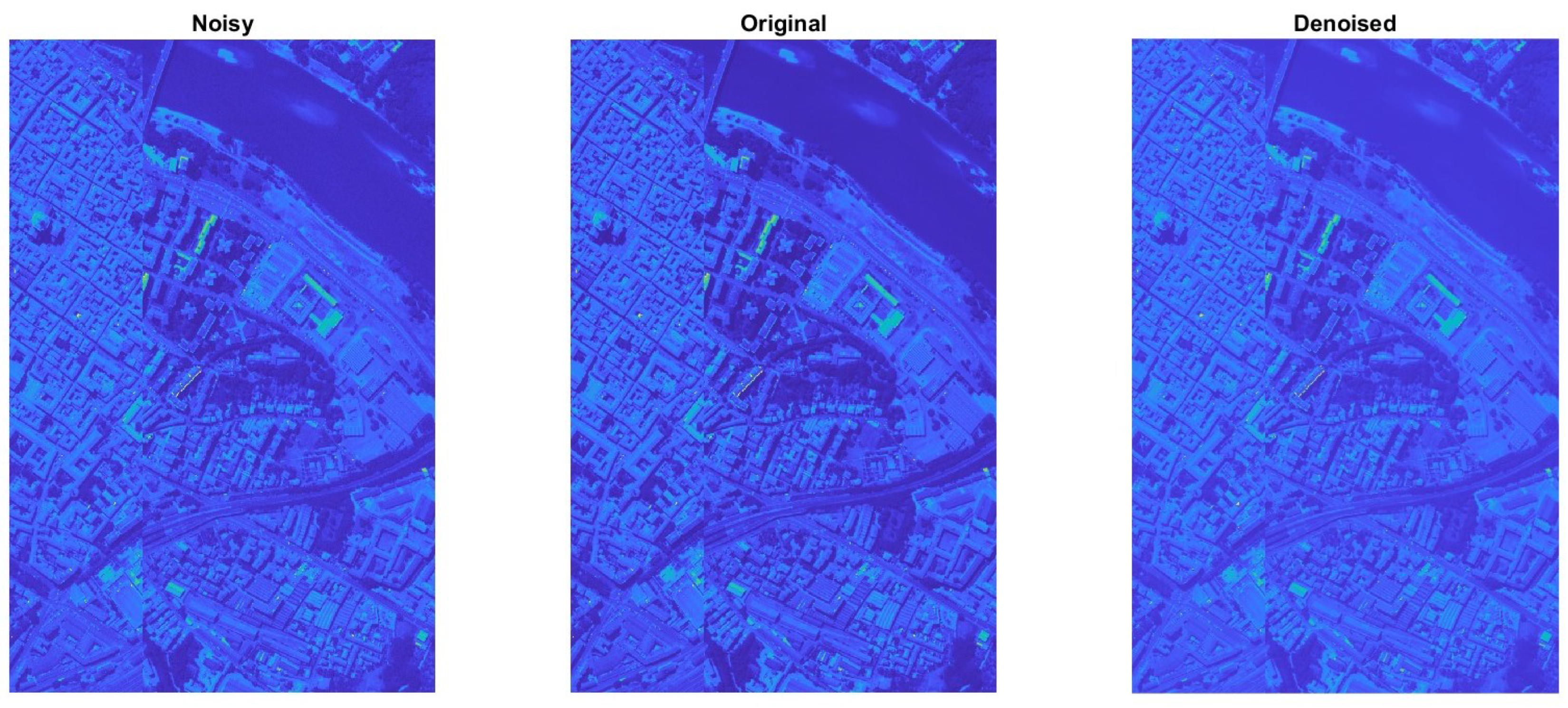
The result of applying LRMR with the optimized parameter setting is shown in Figure 18.

4. Discussion

We note that parameter tests on other different hyperspectral image data sets may provide different parameter settings. Hence, we advise researchers to perform a parameter study for the initial values in the LRMR method setup for a new test set. A problem-specific parameter configuration is suggested, and it was a goal of this work to highlight and provide a sample analysis as a model for other tests.
We computed the nonlinear optimization and the main analysis results in MATLAB. A comparison between the computational costs of MATLAB and Python was presented for the integer-valued parameters. The overall behavior of the algorithms is the same in MATLAB and Python. However, the computational times are significantly larger in Python. The reason is the efficient storing and processing of matrix–vector operations in MATLAB. The analysis of computational times is important for applications where the data budget is limited or where the data have to be processed in real-time (therefore, for real-time decision making). It was important to show the similar behavior in relative terms for both implementations—MATLAB and Python—and to discuss the implementation issues that may occur. We observed stable behavior for each implementation, and the relative behavior was the same.
Regarding future work, other optimization methods can be applied in order to select the optimized initial values for p. We have applied the Broyden–Fletcher–Goldfarb–Shanno (BFGS) quasi-Newton method [19,20,21,22] as an alternative to nonlinear optimization. However, the method always stopped after two iteration steps. Alternatively, the use of a machine learning approach might provide additional parameter optimization results and a more efficient optimization approach to choosing p. This would require access to or the creation of a large data set in order to secure efficient training and testing of the machine learning algorithm. However, this is beyond the scope of this article and is ongoing work of the author.

5. Conclusions

We address parameter analysis and optimization yield improvement of hyperspectral images with regard to the PSNR. We present a detailed analysis with respect to the initial parameters of the LRMR method for different data test sets; however, we focus on the Indian Pines data set. The approach of this work studying parameter optimization for LRMR’s initial parameters is new and has not been presented in this way earlier. The analysis provides new insights into the flexibility and boundaries of the method.

Funding

This research was funded by the Regional Council of Central Finland/Council of Tampere Region and European Regional Development Fund as part of the coADDVA—ADDing VAlue by Computing in Manufacturing projects of Jamk University of Applied Sciences.

Institutional Review Board Statement

Not applicable.

Informed Consent Statement

Not applicable.

Data Availability Statement

All data sets are openly available: Indian Pines [16], Pavia Centre [17], and Pavia University [17].

Conflicts of Interest

The author declares no conflict of interest.

Abbreviations

The following abbreviations are used in this manuscript:
HSIhyperspectral imaging
LRMRlow-rank matrix recovery
GoDecGo Decomposition
PSNRpeak signal-to-noise ratio
BFGSBroyden–Fletcher–Goldfarb–Shanno

References

  1. Mandelbrot, B.B. A fast fractional Gaussian noise generator. Water Resour. Res. 1971, 7, 543–553. [Google Scholar] [CrossRef]
  2. Majumdar, A.; Ansari, N.; Aggarwal, H.; Biyani, P. Impulse denoising for hyper-spectral images: A blind compressed sensing approach. Signal Process. 2016, 119, 136–141. [Google Scholar] [CrossRef]
  3. Shen, H.; Zhang, L. A MAP-based algorithm for destriping and inpainting of remotely sensed images. IEEE Trans. Geosci. Remote Sens. 2009, 47, 1492–1502. [Google Scholar] [CrossRef]
  4. Rogass, C.; Mielke, C.; Scheffler, D.; Boesche, N.K.; Lausch, A.; Lubitz, C.; Guanter, L. Reduction of uncorrelated striping noise—Applications for hyperspectral pushbroom acquisitions. Remote Sens. 2014, 6, 11082–11106. [Google Scholar] [CrossRef]
  5. Sun, L.; Cao, Q.; YChen, Y.; Zheng, Y.; Wu, Z. Mixed Noise Removal for Hyperspectral Images Based on Global Tensor Low-Rankness and Nonlocal SVD-Aided Group Sparsity. IEEE Trans. Geosci. Remote Sens. 2023, 61, 1–17. [Google Scholar] [CrossRef]
  6. Ghamisi, P.; Yokoya, N.; Li, J.; Liao, W.; Liu, S.; Plaza, J.; Rasti, B.; Plaza, A. Advances in hyperspectral image and signal processing: A comprehensive overview of the state of the art. IEEE Geosci. Remote Sens. Mag. 2017, 5, 37–78. [Google Scholar] [CrossRef]
  7. Rasti, B.; Scheunders, P.; Ghamisi, P.; Licciardi, G.; Chanussot, J. Noise reduction in hyperspectral imagery: Overview and application. Remote Sens. 2018, 10, 482. [Google Scholar] [CrossRef]
  8. Singh, S.; Suresh, B. Role of hyperspectral imaging for precision agriculture monitoring. ADBU J. Eng. Technol. 2022, 11, 1–5. [Google Scholar]
  9. Calin, M.A.; Calin, A.C.; Nicolae, D.N. Application of airborne and spaceborne hyperspectral imaging techniques for atmospheric research: Past, present, and future. Appl. Spectrosc. Rev. 2021, 56, 289–323. [Google Scholar] [CrossRef]
  10. Peyghambari, S.; Zhang, Y. Hyperspectral remote sensing in lithological mapping, mineral exploration, and environmental geology: An updated review. J. Appl. Remote Sens. 2021, 15, 031501. [Google Scholar] [CrossRef]
  11. Qian, S.E. Hyperspectral satellites, evolution, and development history. IEEE J. Sel. Top. Appl. Earth Obs. Remote Sens. 2021, 14, 7032–7056. [Google Scholar] [CrossRef]
  12. Wolfmayr, M.; Pölönen, I.; Lind, L.; Kašpárek, T.; Penttilä, A.; Kohout, T. Noise reduction in asteroid imaging using a miniaturized spectral imager. SPIE Sensors Syst. Next-Gener. Satell. XXV 2021, 11858, 121–133. [Google Scholar]
  13. Zhang, H.; He, W.; Zhang, L.; Shen, H.; Yuan, Q. Hyperspectral image restoration using low-rank matrix recovery. IEEE Trans. Geosci. Remote Sens. 2013, 52, 4729–4743. [Google Scholar] [CrossRef]
  14. Zhou, T.; Tao, D. Godec: Randomized low-rank & sparse matrix decomposition in noisy case. In Proceedings of the 28th International Conference on Machine Learning, ICML 2011, Bellevue, WA, USA, 28 June–2 July 2011; pp. 33–40. [Google Scholar]
  15. Lagarias, J.C.; Reeds, J.A.; Wright, M.H.; Wright, P.E. Convergence Properties of the Nelder-Mead Simplex Method in Low Dimensions. SIAM J. Optim. 1998, 9, 112–147. [Google Scholar] [CrossRef]
  16. Purdue University Research Repository. Indian Pines Data Set. Available online: https://purr.purdue.edu/publications/1947/1 (accessed on 12 December 2022).
  17. Pavia Centre and University Data Sets; Gamba, P. Telecommunications and Remote Sensing Laboratory, Pavia University. Available online: https://www.ehu.eus/ccwintco/index.php/Hyperspectral_Remote_Sensing_Scenes#Pavia_Centre_and_University (accessed on 12 December 2022).
  18. Wright, J.; Ganesh, A.; Rao, S.; Peng, Y.; Ma, Y. Robust principal component analysis: Exact recovery of corrupted low-rank matrices via convex optimization. In Proceedings of the Advances in Neural Information Processing Systems, Vancouver, BC, Canada, 7–10 December 2009; p. 22. [Google Scholar]
  19. Broyden, C.G. The Convergence of a Class of Double-Rank Minimization Algorithms. IMA J. Appl. Math. 1970, 6, 76–90. [Google Scholar] [CrossRef]
  20. Fletcher, R. A New Approach to Variable Metric Algorithms. Comput. J. 1970, 13, 317–322. [Google Scholar] [CrossRef]
  21. Goldfarb, D. A Family of Variable Metric Updates Derived by Variational Means. Math. Comput. 1970, 24, 23–26. [Google Scholar] [CrossRef]
  22. Shanno, D.F. Conditioning of Quasi-Newton Methods for Function Minimization. Math. Comput. 1970, 24, 647–656. [Google Scholar] [CrossRef]
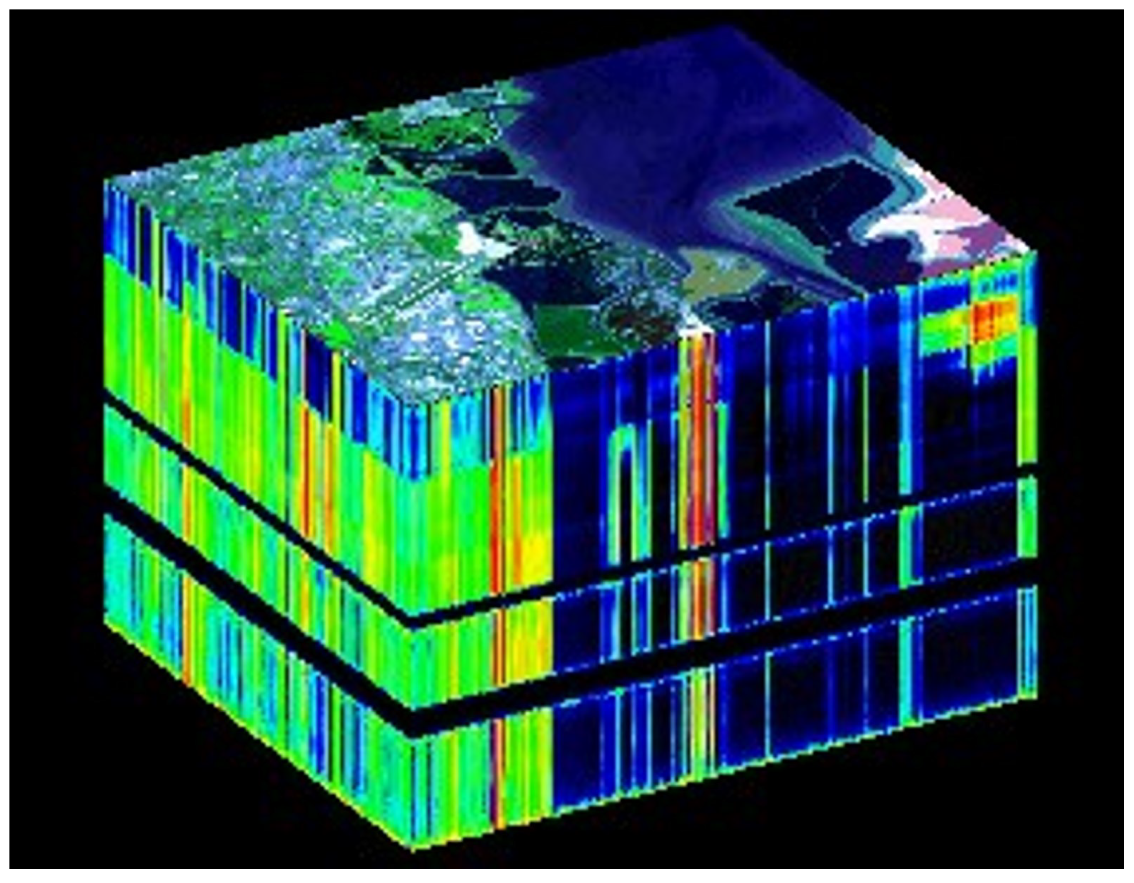
Figure 1. An example of a hyperspectral data cube (courtesy of NASA/JPL-Caltech).
Applsci 13 09373 g001
Figure 2. The Indian Pines data set displayed for six different spectral reflectance bands: 1, 50, 80, 130, 180, and 220.
Applsci 13 09373 g002
Figure 3. The Pavia Centre data set displayed for spectral reflectance bands 1, 50, and 102.
Applsci 13 09373 g003
Figure 4. The Pavia University data set displayed for spectral reflectance bands 1, 50, and 103.
Applsci 13 09373 g004
Figure 5. The noise removal performance of LRMR on a noise-corrupted spectral band for the Indian Pines data set. The image is restored efficiently.
Applsci 13 09373 g005
Figure 6. PSNR plot for different values of r.
Applsci 13 09373 g006
Figure 7. CPU time plot for different values of r.
Applsci 13 09373 g007
Figure 8. PSNR plot for different values of s.
Applsci 13 09373 g008
Figure 9. CPU time plot for different values of s.
Applsci 13 09373 g009
Figure 10. PSNR surface plots for different r and s intersects.
Applsci 13 09373 g010
Figure 11. PSNR plot for different values of b.
Applsci 13 09373 g011
Figure 12. CPU time plot for different values of b.
Applsci 13 09373 g012
Figure 13. The function values of the iteration steps of the nonlinear optimization Nelder–Mead simplex algorithm with respect to p for the Indian Pines data set and starting value p = 0.15 .
Applsci 13 09373 g013
Figure 14. PSNR plot for analyzing different starting values of p.
Applsci 13 09373 g014
Figure 15. CPU time plot for different values of p.
Applsci 13 09373 g015
Figure 16. LRMR result computed on the Indian Pines data set for the optimized parameter settings.
Applsci 13 09373 g016
Figure 17. LRMR result computed on the Pavia Centre data set for the optimized parameter settings.
Applsci 13 09373 g017
Figure 18. LRMR result computed on the Pavia University data set for the optimized parameter settings.
Applsci 13 09373 g018
Table 1. The PSNRs, gradients of PSNR, and the CPU times in seconds for computing the denoised cubes for different values of r in MATLAB t M a t l a b and Python t P y t h o n .
rPSNR∇PSNR t M a t l a b t P y t h o n
120.9914.7014.3195.15
235.6910.0218.3785.57
341.025.0420.32108.98
445.773.2821.63107.42
547.581.4521.84109.01
648.670.9424.70108.22
749.450.7626.32115.23
850.190.6927.23112.48
950.830.6128.06114.21
1051.420.6028.92116.79
1152.030.6131.49117.49
1252.650.5330.3599.18
1353.100.4430.96100.97
1453.520.3832.62103.88
1553.870.3333.1297.06
1654.190.3134.03111.33
1754.490.3135.12113.62
1854.810.2835.81104.27
1955.060.2436.22121.06
2055.280.2238.06125.18
Table 2. The PSNR, the CPU times in seconds, and the gradient of CPU times for computing the denoised cubes for different values of s in MATLAB t Matlab as well as the CPU times in Python t Python .
sPSNR t Matlab t Matlab t Python
149.61951.11−706.383793.27
249.62244.72−420.411007.87
349.56110.29−90.82481.01
449.5863.09−30.02301.01
549.6150.24−16.93193.88
649.5729.22−10.62178.32
749.4629.00−1.63114.31
849.4825.96−7.63100.41
949.4513.741.54139.66
1049.4029.047.71112.07
1149.4729.16−10.48111.66
1249.198.08−7.71137.42
1349.3413.749.0153.73
1449.2326.11−1.90100.47
1549.179.941.5338.31
1649.2429.181.85111.84
1749.1713.63−12.6052.35
1848.973.987.81178.98
1949.0529.255.95114.47
2048.8315.88−13.3660.94
Table 3. The CPU times in seconds for computing the denoised cubes for different values of b in MATLAB t Matlab and Python t Python .
bPSNR t Matlab t Python
1550.1411.0148.13
1649.9611.5883.56
1749.8726.39102.33
1849.7326.41124.62
1949.6226.23122.86
2049.4224.71127.33
2149.3624.2997.29
2249.2323.3792.63
2349.1623.04102.33
2449.0721.16179.84
2548.88127.72257.69
Table 4. The final function values for the minimization problem (the negative PSNR values) and the corresponding parameter value p final for different starting values p 0 . Clearly, local minima are approached. Based on the Indian Pines data set.
p 0 −PSNR p final
0.015−49.9902560.014977
0.05−49.8877820.047813
0.15−49.5034830.143438
0.5−49.4765120.596875
1.−49.6168820.975000
1.5−49.7507811.818750
Disclaimer/Publisher’s Note: The statements, opinions and data contained in all publications are solely those of the individual author(s) and contributor(s) and not of MDPI and/or the editor(s). MDPI and/or the editor(s) disclaim responsibility for any injury to people or property resulting from any ideas, methods, instructions or products referred to in the content.