NoisenseDB: An Urban Sound Event Database to Develop Neural Classification Systems for Noise-Monitoring Applications

Abstract

The use of continuous monitoring systems to control aspects such as noise pollution has grown in recent years. The commercial monitoring systems used to date only provide information on noise levels but do not identify the noise sources that generate them. The identification of noise sources is an important aspect in order to apply corrective measures to mitigate the noise levels. In this sense, new technological advances like machine listening can enable the addition of other capabilities to sound monitoring systems such as the detection and classification of noise sources. Despite the increasing development of these systems, researchers have to face some shortcomings. The most frequent ones are on the one hand, the lack of data recorded in real environments and on the other hand, the need for automatic labelling of large volumes of data collected by working monitoring systems. In order to address these needs, in this paper, we present our own sound database recorded in an urban environment. Some baseline results for the database are provided using two original convolutional neural network based sound events classification systems. Additionally, a state of the art transformer-based audio classification system (AST) has been applied to obtain some baseline results. Furthermore, the database has been used for evaluating a semi-supervised strategy to train a classifier for automatic labelling that can be refined by human labellers afterwards.

1. Introduction

Community noise (also called environmental, urban, or residential noise) is one of the main problems that cause a negative impact on health. Since the 1990s, the World Health Organization (WHO) has developed different guidelines to serve as a basis for the standards in the management of environmental noise. In the European Union, since the publication of the Environmental Noise Directive 2002/49/EC (END) [1], the European Member States have developed their own legislation to reduce the noise levels to which their populations are exposed. Although considerable efforts have been made to reduce noise levels, the latest report published by the European Environmental Agency [2] indicates that this has not been accomplished. This concern to control and manage noise pollution in general, has resulted in the advent of smart cities, which have boosted the deployment of monitoring systems.

Monitoring systems are effective tools for the evaluation and management of acoustic pollution, which complement noise strategic maps, the main tool currently in use. Noise maps have certain limitations for noise-source assessment: only a few noise sources are taken into account and they use averaged data over long periods for calculating the acoustic emission of the sources. The use of monitoring systems would overcome those limitations and contribute to obtain a more realistic approximation of noise levels, especially in cities. The data provided using real-time monitoring systems allow other types of analysis, such as the characterization of behavioural patterns and detection of high-level short-duration noise events that can cause annoyance and negative health effects.

However, current monitoring systems have the downside of not identifying the sound sources that generate the noises, making it difficult to take corrective actions. This problem arosed in one of the earliest research projects on the use of sensors in a continuous monitoring system for evaluating noise pollution, conducted in Palma de Mallorca [3]. This project’s objective was to assess how sound pressure levels (SPL) and particulate matter (PM10) particles produced by port activity were related to one another. They were unable to establish a clear connection between the noise levels recorded and the noise sources responsible for them. Sound-classification techniques can be used to solve this issue, making it possible to identify the noise source responsible for a specific sound event.

New approaches to age-old problems in the analysis and processing of sound signals, like speech recognition and sound categorization, have been made possible by the application of machine learning techniques. Machine learning is a set of techniques that allow computer programs to automatically improve doing a task through experience. These systems are able to extract and identify complex patterns in the data (in our case sound) that could not be processed using traditional processing and handcrafted features. More specifically, the term Machine Listening or Machine Audition [4], encompasses the study of techniques and systems that allow computers to automatically identify sounds as humans do. There are many uses for machine listening, but two of the most important ones are the sound event detection [5], which identifies the beginning and end of a sound event in a recording, and audio classification which aims to categorize or label a recording. There are many application fields for audio classification, including the categorization of environmental sounds (both urban and nature) [6], bioacoustics signal classification and detection [7,8] and the classification of urban sound events in noise monitoring systems [9,10,11], our research topic.

A lot of the research in this area has been promoted by the Detection and Classification of Acoustic Scenes and Events (DCASE) community, which has been organising challenges and workshops for the last years. The aim of the DCASE community is the support development of computational scene and event analysis methods by providing public datasets [12,13], and giving researches the opportunity to continuously compare different approaches on the same datasets, using consistent performance measures. The challenges “Urban Sound Tagging with Spatiotemporal context”, organized in 2020, and “Acoustic Scene Classification”, organized in 2021 [14], had important contributions in the sound-classification area.

For these classification tasks, the majority of researchers use deep neural network (DNN) architectures that perform rather well as they have the ability to extract discriminative feature representations. The most popular architectures are based in Convolutional Neural Networks (CNN) [6,15,16]. Some other researches, motivated by the fact that the CNNs do not learn long-term dependencies, propose solutions based on CNNs combined with Recurrent Neural Networks (RNN) [17,18,19]. However, the RNNs suffer from the vanishing gradient problem. To overcome this problem the ResNets [20,21,22] were introduced, as they use residual blocks that enable training a large number of layers. More recently, transformer architectures purely based on attention mechanisms [23,24,25] and hybrid architectures combining transformers with RNNs [26] and ResNets [27], have been proposed. Most of the systems apply data augmentation and transfer learning techniques. Some other systems propose the fusion of different classifiers [28,29,30,31] and features [32,33].

Good outcomes depend on the network architecture selected, which is influenced by the problem to be solved, the quantity and quality of the data available and other factors. Despite the widespread use of DNNs, researchers are still facing some challenges as the lack of annotated data for certain tasks, especially for real-world applications. The ESC dataset [34], UrbanSound8k [35], AudioSet [36], and the more recently released SONYC-UST [13] and SONYC-USTv2 [37] datasets are the most popular and openly accessible datasets that are frequently utilized in the development and evaluation of urban sound classification systems. The ESC dataset consists of three parts. Two of them, ESC-10 and ESC-50, comprise a labelled set of 10 and 50 classes of different environmental sounds while the third part, ESC-US, is a set of non-labelled data. All clips were extracted from the public field recordings available in the Freesound project [38]. UrbanSound8k contains labelled recordings for 10 classes of urban sounds, also extracted from the Freesound project. In turn, AudioSet corpus consists of labelled sounds from different sources (domestic, environmental, nature, music, ...) drawn from YouTube.

The majority of the aforementioned datasets have the drawback of not having been recorded for monitoring urban noise. SONYC project [9], addresses this problem, deploying a number of noise monitoring sensors for collecting data. The aim of collecting the data was to develop a classification system for a specific task, namely to confirm that the complaints made by residents about violations of the noise code of New York City were true. SONYC-UST and SONYC-USTv2 are multi-label datasets for urban sound tagging that comprise a fine labelled set of 23 classes that are grouped into 8 coarse classes with more general descriptors. The main difference between them is that the latter includes spatio-temporal context information about the recording event. More recently, the so called SINGA-PURA database has been published [39] following the structure of SONYC-UST V2 taxonomy and expanding some classes in more detail.

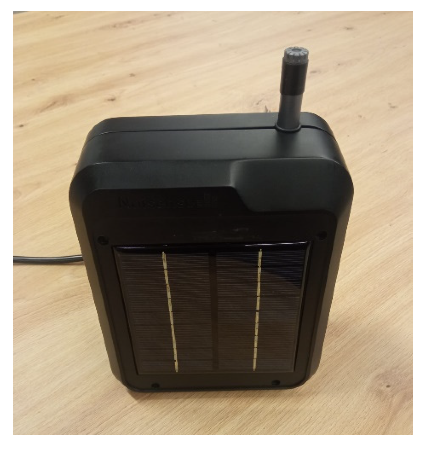
In any case, more datasets with samples from real application scenarios are still needed in this area. In this line, we present a novel audio database, the so called NoisenseDB, with real urban sound events intended to be used in sound-classification tasks. The recording of this database was performed by deploying a continuous monitoring system developed by the company NOISMART in real urban locations.

Another problem that researchers have to face is how to label the great amount of acquired material generated by a sensor recording continuously. Manual identification of sound sources in large audio files takes up a significant amount of research time. Some projects have used crowdsourcing [40], where volunteers tagged the audio files using internet platforms like Zooniverse. Since this method of labelling often produces low-quality results, other approaches, such as Active Learning [41] or Semi Supervised Learning [42] are very interesting. These methods are grounded on the idea that by means of actively choosing the most accurately predicted data, algorithms can increase their performance while utilizing less training data. Pseudo-labelling [43], also called self-training [44] is one of the techniques that has garnered the greatest interest in recent years. This method, involves training a classifier on labelled data, predicting the labels for the unlabelled data and retraining the model adding confident predicted data to the training data.

In this paper, besides presenting the new NoisenseDB, we propose several state-of-the art urban sound events classification systems. We also analyse the feasibility of a semi-supervised training approach to cope with the labelling of the large amounts of data produced by such continuous monitoring systems.

This paper is organized as follows: Section 2 describes the data-acquisition device and recording locations; Section 3 explains the creation of the NoisenseDB database, its taxonomy and structure; Section 4 introduces the tested sound event classification systems; Section 5 shows the experimental results using these systems with NoisenseDB. Finally, some conclusions are presented in Section 6.

2. Audio Data Acquisition

2.1. Recording Device

The audio of the database was recorded using a noise-monitoring sensor developed by NOISMART, which includes a recording module (Figure 1). The noise-measuring sensor registers the ambient sound pressure level (SPL) and can also record audio clips. It is based on a commercial printed circuit board (PCB) and includes an omnidirectional pattern microphone with a frequency response of 20 Hz–20 kHz that replaces the standard micro-electro-mechanical (MEM) microphone on the PCB. The microphone is externally mounted.

Each audio file was recorded in wav format with constant gain settings, mono configuration, and a sampling rate of 48 kHz and 16-bit coding.

2.2. Recording Locations

The recording of the database was carried out placing the device at two different locations in order to capture different sound sources. In both locations, the device was mounted on the façade of a building at an approximate height of 4 m over the street level.

The first location was in the city centre of Algorta (Biscay). It was chosen with the aim of collecting sounds related to traffic, street works and usual sounds of an urban area. The equipment was in use during 31 days between May and June of 2021, recording 600 h of data.

The second location was in Portugalete (Biscay), and it was intended to record urban sounds related to leisure. Between the end of June and the beginning of August 2021, the device was deployed for 31 days, capturing 687 h in total. NoisenseDB was built from selected audio segments from this large set of recordings, as it is explained in the next section.

3. NoisenseDB

3.1. Sound Event Extraction

Obviously, not all the recorded data (more than 1200 h) contained meaningful and identifiable sound events, and thus, we had to establish an efficient way to extract these interesting sound events for the creation of the database. The criteria was to use the SPL measures to determine where these sound events were, assuming that sounds with higher SPL will be easier to identify and also easier for an automatic classification system to learn.

From the total of the recorded hours, we extracted a set of variable-length audio clips corresponding to the sound events that registered a peak level equal or greater than 71 dB(A) and kept above 60 dB(A) during at least 3 consecutive seconds.

The segmentation of the audio clips with sound events in the original recordings was done taking 3 s before the SPL threshold was surpassed. This criterion was applied because for some events the onset of the noise gives important information about its source. The downside is that this additional period can introduce noise into the system since other unlabelled sound events may appear.

The resulting audio clips have variable length depending of the sound event and make a total of 692 sound clips. A single trained person labelled all the audio clips, assigning one single label to the entire audio clip. This is known as monophonic labelling, and implies the assumption that each audio clip included just one type of sound. Thus, sometimes we will use event as synonym for audio clip in the following sections. Actually, sometimes two different audio events occur within the same clip. This happened in the 20% of the clips, especially when mixing “Music” and “Voice” categories. In these cases, the clip is labelled with the most prominent of both events. The criterion is to use first the length of each event and, if their length is similar, their intensity.

Exceptionally, in the case of very scarce sound events (dog barking and impact sounds), the annotation criteria has been to prioritise these events for labelling, even though other possible sounds in the clip can even last longer. Thus if any of these events appear in the clip the whole clip is assigned to that event.

3.2. NoisenseDB Taxonomy

In order to define our taxonomy, we analysed the semantic classification of sounds carried out by J. Salomon et al. [35]. They created an extensive taxonomy, with more than 50 sound events, distributed in different levels with four higher-level categories. The SONYC project defined a simpler taxonomy with just two levels [13]. Both these taxonomies have more types of events than our recorded data, so we defined a simpler taxonomy.

NoisenseDB taxonomy can be seen in

Table 1. NoisenseDB Taxonomy.

Coarse Categories	Fine Categories
traffic	car
	motorbike
	cleaning truck
human	voice
	music
nature	dog
	storm
mechanical	impact
	machinery

. It consists of nine different (fine) categories gathered in four higher-level (coarse) categories, grouping those sound events with similar origin. This taxonomy was used for labelling the NoisenseDB.

3.3. Database Structure

NoisenseDB is divided into two datasets, using the peak SPL of the event as criterion. The main one is called supervised dataset (SD) and it is designed for supervised learning. It is composed of the audio clips of sound events with highest SPLs, namely greater than or equal to 72 dB(A). Its 432 audio clips are distributed in 5 folds that can be used as training, validation and evaluation partitions in cross validation experiments. The audio clips, and consequently the sound events, are never divided into different folds. The audio clips have been distributed in folds trying to keep a balance in the total duration of the audio samples for each class. For the class “Machinery” this approach was not possible due to the small number of events and their different duration, and in this case, the distribution was done keeping the number of events balanced in each fold independently of their duration.

The second dataset, the so-called unsupervised dataset (UD), is intended to be used as evaluation set for unsupervised learning. It included 260 audio clips of sound events with the highest SPL values equal or greater than 71 dB(A) and less than 72 dB(A).

The distribution of sound events per class is shown in

Table 2. SD and UD events length and distribution by class. Length in seconds.

Supervised Dataset (SD)						Unsupervised Dataset (UD)
Categories	Total	Min	Max	Average	Total	Total	Min	Max	Average	Total
	Length	Length	Length	Length (±σ)	Events	Length	Length	Length	Length (±σ)	Events
car	1795	6	123	17.1 ± 17.4	105	918	6	56	14.8 ± 8.4	62
motorbike	2240	6	123	21.5 ± 20.1	104	511	8	39	14.6 ± 5.9	35
cleaning-truck	1164	20	123	77.6 ± 38.6	15	441	6	123	55.1 ± 39.7	8
voice	7004	6	123	71.4 ± 49	98	11420	7	123	88.5 ± 43.5	129
music	4813	6	123	104.6 ± 34	46	21	6	15	10.5 ± 4.5	2
dog	183	7	29	13. ± 7.1	14	128	6	24	12.8 ± 6.1	10
storm	831	6	123	51.9 ± 48.8	16	11	11	11	11 ± 0	1
impact	184	6	26	12.3 ± 6.2	15	79	6	20	11.3 ± 4.3	7
machinery	501	6	123	26.4 ± 35.4	19	232	6	123	38.6 ± 39.3	6

along with some statistics related to their length. The minimum possible length is 6 s corresponding to 3 s over the SPL threshold limit plus the previous 3 s. The maximum length is also bounded to 3 + 120 s.

Table 2 shows that the classes are heavily unbalanced both in the SD and UD sets. In the SD part, five categories have less than 20 events, while the others have more than 40. The length of the events is also very different. The categories of “Impact” and “Dog” are really scarce both in terms of number of events and length of the samples. In the UD part the imbalance is still worse but in this case the less represented ones are “Storm” and “Music”. We have not taken any measure to reduce the original imbalance of the database, because the aim of this work was to obtain a database representing the real-world difficulties of the urban sound events classification task. Thus, the database contains all the sound events that have been registered during the two months of the monitoring period.

4. Sound Event Classification Systems

We have tested three different DNN architectures to provide some baseline classification results for the database. Two of them are novel systems proposed by us, which are based on convolutional neural networks (CNNs). The third one is a transformer based neural network, the so called, Audio Spectrogram Transformer, proposed in [23] and it is included to provide a reference to allow comparison with a state of the art system. They are briefly described below.

4.1. CNN-Based Models

The first two systems that we propose are based on a classifier fed by the combination of audio features extracted using CNNs and embeddings of the audio segments obtained using OpenL3, an embedding model trained using the environmental subset of AudioSet video database [45]. Two systems with different CNN architectures have been tested, one based on convolutional blocks and the other one based on ResNets [21]. Each system will be described with more detail in the following subsections. Figure 2 shows a diagram of both systems.

4.1.1. Audio Processing and Data Augmentation

Due to the varying length of each sound clip in the database, the audio files have been cut into fixed length analysis fragments of 1 s, with 0.5 s hop size. The original sampling frequency of 48 kHz has been kept. All the fragments from the same audio clip inherit the label of the whole clip, so all of them have the same label. All the programming for processing and implementing the classifiers has been done using Python as programming language.

To feed the CNN branch, the log-Mel spectrogram of each fragment is calculated using the Librosa [46] library, with 128 Mel filters and a window length of 21 ms and a frame shift 10.5 ms (resulting in 94 frames). These log-Mel spectrograms are used as input to the convolutional layers.

The other branch uses OpenL3 embeddings. These embeddings are obtained using Mel-spectrograms calculated as explained before as an input for the embedding model which returns an embedding vector of 512 values.

Mixup is used as an augmentation technique for the training data. This technique [47] generates a weighted combination of random pairs of vectors from the training data with their corresponding labels. The input vector pairs (both log-Mel spectrograms and embeddings) are combined with a weighting value within the [0, 1] range, sampled from a Beta distribution with α = 0.4, and the one-hot encoded labels are also combined applying the same weight.

4.1.2. Architecture of the Classifiers

Both proposed novel systems take the input data described before, but the difference between them is the CNN branch that processes the log-Mel spectrogram part. The first architecture, Figure 2a, uses three blocks of convolutional layers (ConvBlock), while the second one, Figure 2b, uses a ResNet. They are described in detail in the following subsections.

For both systems, the output of the CNN branch was concatenated with the OpenL3 embeddings. The resulting combined parameter vector was used as input for a fully connected layer with 128 neurons with 50% dropout. Finally, a softmax layer was used to produce the classification scores. The systems were implemented using the Keras API.

ConvBlock Branch

The first of the systems used a CNN branch based on three convolutional blocks. Each convolutional block (Figure 3) consisted of a 2D convolutional layer with a kernel size of (3 × 3), and a (2,2) stride. After each convolutional layer, we applied batch normalization, ReLU activation and max pooling with a pool size of (3 × 2) and a stride of (1,2). Each of the blocks had a decreasing number of convolutional filters (f): 256, 128 and 64.

ResNet Branch

The CNN branch of the second system was based on a ResNet. We developed this architecture based on ResNet50 [21] with some design and implementation details inspired by [48].

The ResNet branch (shadowed in grey in Figure 2b) consisted of an input stage, 10 groups of convolutional and identity blocks (CBIB) and a MaxPooling layer. The input stage Figure 2b consisted of a 2D convolutional layer with 256 filters, a kernel size of (3 × 3) and a stride of (1,1). After the convolutional layer, we used batch normalization, ReLU activation and a MaxPooling layer with a pool size of (2,2) and the same stride size.

After the input stage, 10 CBIB blocks were stacked. Each CBIB block consisted of a Convolutional Block (CB) followed by an Identity Block (IB). The number of blocks, the number of layers and their respective number of filters were chosen after carrying out different tests in which we modified these hyperparameters. Those experiments were performed in previous works with other datasets and in this paper, we presented the architectures that obtained the best results. The CB block, Figure 4, consisted of three 2D convolutional layers on the main branch and a shortcut with one 2D convolutional layer. The Conv2D layers of the main branch had a decreasing number of filters (f1, f2, f3) with (256, 128, 64) values. The first Conv2D layer and the shortcut had a different stride (s,s) depending on the position of the CBIB block in the stack, while the rest of the layers had a fixed value of (1,1). The stride (s) values assigned to the CB blocks were (2,2) for the 3rd, 6th and 9th CBIB blocks and (1,1) for the rest of them. The stride values followed the original ResNet50 [21], but without downsampling on the 2nd, 5th and 8th CBIB blocks. The shortcut consisted of a Conv2D with the same number of filters as the third Conv2D (64), a kernel size of (1 × 1) and a stride of (s,s), which was 1 or 2 depending on the number of blocks, as explained before. The outputs of the CB blocks and the shortcut branch were added to use them as the input of the identity block, as shown in Figure 4.

The configuration of the identity block is similar to the convolutional block, except for the stride value, which is 1 for all layers; and the shortcut, where there is no Conv2D layer.

4.2. Audio Spectrogram Transformer

We have also tested the Audio Spectrogram Transformer (AST) architecture proposed in [23], a state of the art architecture that provides an independent baseline to compare with our proposed convolutional architectures. This system uses a transformer-based architecture to classify audio signals. Transformers require a great amount of training data, much more than the amount required by CNNs. That is why the AST uses pretrained models. Moreover, since spectrograms can be considered as images, the AST employs cross-modality transfer learning training an initial model using the Vision Transformer (ViT) [49] architecture trained with the ImageNet [50] database. This initial model was retrained with spectrograms from the AudioSet database. This results in the AST-P public model [51] that we have used as pretrained initialization for the training of the network with our database.

The preprocessing of the sound event recordings for the AST was similar to that of the convolutional systems (see Section 4.1.1): the audio files were cut into fixed-length analysis fragments of 1 s, with a 0.5 s hop size, but in this case, as the AST uses pretrained models, the audio files had to be downsampled to 16 kHz. Each fragment was converted into a log-Mel-spectrogram using a Mel filter bank of 128 filters, with a framerate of 10 ms and a window of 25 ms. The outcome was next divided into a set of 16 × 16 patches, which were then linearly projected onto a set of 1D embeddings. Each patch embedding was added to a learnable positional embedding. An additional classification token was appended to the sequence. The resulting sequence was then used as an input to the transformer. Since the AST is designed for classification tasks, it only uses the encoder part of the original transformer architecture [52]. AST uses an encoder that has an embedding dimension of 768, 12 layers, and 12 heads. The output of the encoder of the transformer serves as the audio spectrogram representation. A linear layer with sigmoid activation maps the audio spectrogram representation to a label for classification.

5. Classification Experiments

We used the different parts of the NoisenseDB for two different objectives. First, we used the SD to obtain baseline results for the three DNN classifiers presented in Section 4. Second, we also used the UD of the NoisenseDB to evaluate the feasibility of a semi-supervised learning strategy using convolutional classification systems.

5.1. Evaluation Metrics

Although accuracy is one of the most frequently used metrics to assess the performance of a classification system, it is not suitable if the test database is unbalanced. In those cases, the use of another metric such as recall is recommended. We have used the macro-average recall [53] as main assessment metric. For calculating the macro-average recall, first, the recall is computed for each class (1), and then we average all the recall values of the n (number of classes) to get the macro-average recall (2).

$$Recall\left(R\right)=\frac{True Positives}{True Positives+False Negatives}$$

(1)

$$macro-average recall=\frac{{{\displaystyle \sum }}_{i=1}^{i=n}Ri}{n}$$

(2)

For each of the evaluated architectures, we presented the baseline results in two different ways. The first one calculated the macro average recall at the fragment level, while the second one calculated the metric for the entire sound clip, which was composed of several fragments. For calculating the metrics for the entire audio clip, we used a modified majority voting method.

Normally, in the majority voting method, the predicted output class for the whole audio clip would be the class that has a greater number of predictions for the fragments of that audio. Taking into account the criteria that we used during the labelling phase, especially for “Dog” and “Impact” categories, we made some modifications on the majority voting method. This modification consisted on assigning “Dog” or “Impact” category to the whole audio clip if just one frame is classified as ”Dog” or “Impact”.

5.2. Classification of the Supervised Dataset

For the SD classification, we used five-fold cross validation using the distribution of the database shown in Table 2. For each iteration, we used one fold for validation and the remaining folds for training (approx. 80–20%). The convolutional classification systems (ConvBlock and ResNet) were trained using an Adam optimizer with a learning rate of 1 × 10⁻⁴. L2 regularization with a factor of 1 × 10⁻⁵ was also used. We also applied a learning rate reduction of 0.5 if the validation loss metric did not improve after 4 epochs. The values of the aforementioned parameters were chosen from previous experiments carried out with different databases. The AST model was trained using the Adam optimizer for 25 epochs with an initial learning rate of 1 × 10⁻⁵ and decreasing it with a factor of 0.85 every epoch after the 5th one. These are the recommended parameters of the original architecture.

5.2.1. Baseline Results for Coarse Classification

We computed the metrics to evaluate the performance for the four-category taxonomy. We have calculated the results both at fragment level and for the entire audio clip. We applied majority voting without modification as “Dog” and “Impact” labels are not present in the four-category taxonomy.

Table 3. Recall values (mean and standard deviation) at fragment level classification averaged through the cross-validation iterations. Data in %.

Category	ConvBlock (m ± σ)	ResNet (m ± σ)	AST (m ± σ)
traffic	94.2 ± 1.9	95.7 ± 2.5	94.7 ± 1.8
human	97.7 ± 0.4	97.9 ± 0.5	97.4 ± 0.8
nature	84.2 ± 4.3	84.7 ± 0.4	86.1 ± 3.4
mechanical	53.9 ± 18.3	53.2 ± 18.4	51.5 ± 11.3
Macro recall	82.5 ± 5.7	82.9 ± 5.6	82.4 ± 2.4

shows the mean and standard deviation of the cross-validation iterations of the recall values (per class and macro-averaged) for each system at fragment level.

Although the differences between the models are not statistically significant (confidence intervals for p > 0.95: ConvBlock 4.9, ResNet 4.9, AST 2.1), ResNet achieves the best overall result.

The results for all the most represented categories are very good for the three systems, but the performance decays for the mechanical sounds category due to the scarcity of training material for this category and the different kind of sounds that are included in it.

Table 4. Recall values (mean and standard deviation) for the entire audio clip classification averaged through the cross-validation iterations. Data in %.

Category	ConvBlock (m ± σ)	ResNet (m ± σ)	AST (m ± σ)
Traffic	97.3 ± 1.7	98.3 ± 0.9	98.6 ± 1.9
Human	83.5 ± 3.1	87.0 ± 4.4	84.9 ± 5.3
Nature	63.3 ± 12.5	60.0 ± 17.0	70.0 ± 12.5
Mechanical	41.4 ± 11.4	29.5 ± 9.2	41.8 ± 15.1
Macro recall	71.4 ± 4.9	68.7 ± 4.4	73.8 ± 5.4

shows the metrics for the entire audio classification. In this task, the overall performance of the systems is worse compared to the fragment classification scores. This is due to several factors: first, the number of audio clips is smaller than the number of frames and this produces greater variability in the results for each iteration. Second, in the classes where frame classification accuracy is worse (e.g., in short, punctual events) the frames correctly classified can be easily outnumbered by frames wrongly classified in other classes. This is the case for “Mechanical” and to a lesser extent for “Nature”. It would be worth evaluating other methods apart from majority voting to see if this performance can be improved. Conversely the classes that have higher accuracy at fragment level are boosted because the majority voting filters out the sporadic fragment-level classification errors.

The results were similar for both ConvBlock and AST in most of the categories, but for ResNet, the performance reduced more due to the fall in the most difficult classes (“Nature” and “Mechanical”). Nevertheless, regarding the macro recall, the difference between the models was not statistically significant (confidence intervals for p > 0.95: ConvBlock 4.3, ResNet 4.3, AST 4.7).

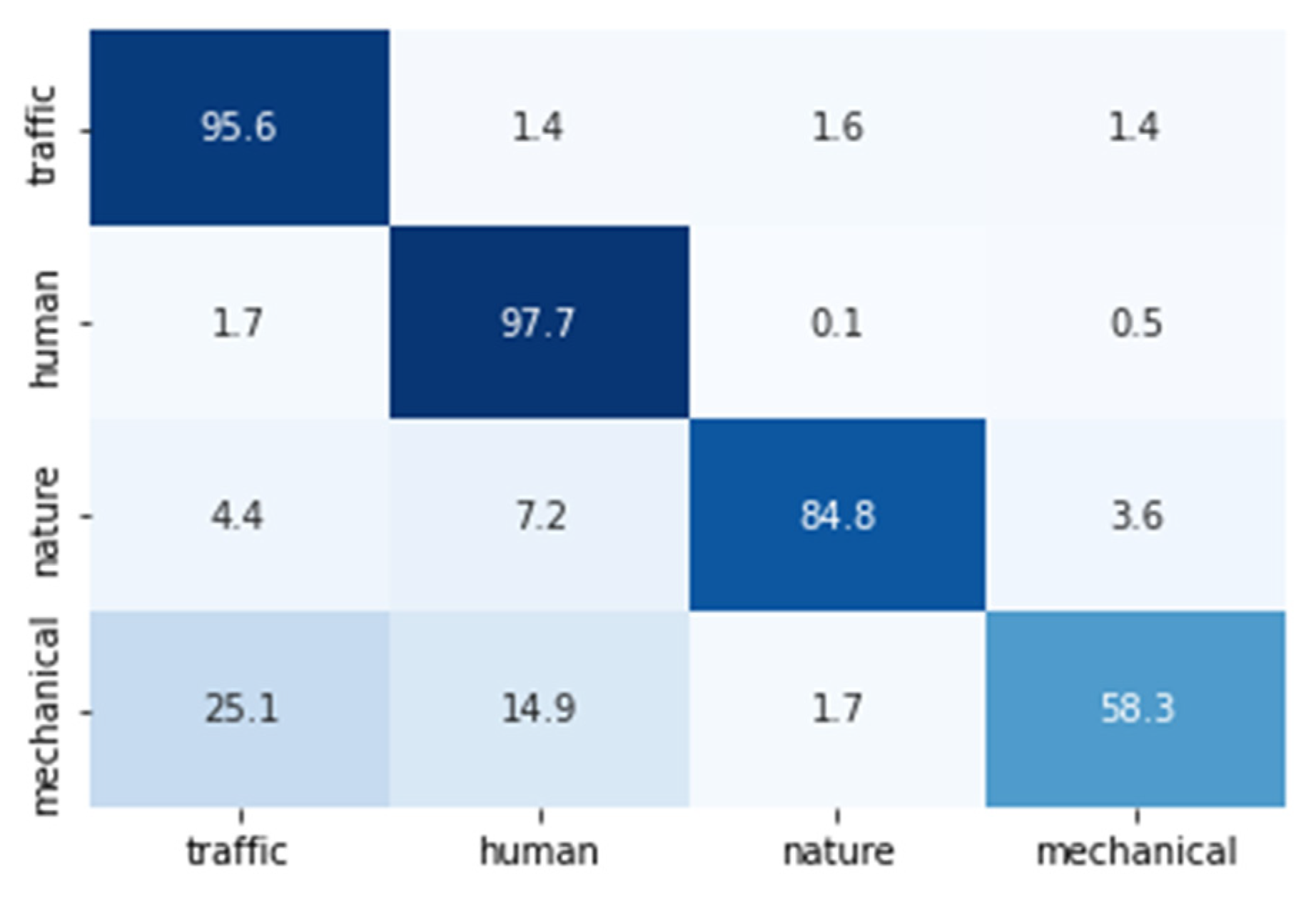
Figure 5 shows the confusion matrix of the ResNet architecture for which we achieved the best results at the fragment level. The rows represent the true labels while the columns represent the predicted ones. The global confusion matrix was calculated considering the classifications obtained in all the iterations by each class and divided by the total number of elements in that class. Darker colors represent the highest scores.

The results were good for all the categories except for the “Mechanical” one, for which 25.1% and 14.9% of the fragments were erroneously classified as “Traffic” and “Human”, respectively. The differences between the values of the diagonal of the confusion matrix (Figure 5) and the values of Table 3, corresponding to the ResNet, were due to the fact that the former was calculated by adding all the classification results for the frames of every iteration, whereas the latter was calculated averaging the recalls of each iteration.

5.2.2. Baseline Results for Fine Label Classification

We also trained the classifiers with the nine-category taxonomy, making decisions both at fragment level and for the entire audio clip. In this last case, we used the modified majority voting for “Dog” and “Impact” categories.

Table 5. Recall values (mean and standard deviation) for fragment-level classification averaged through the cross-validation iterations. Data is in %.

Categories	ConvBlock (m ± σ)	ResNet (m ± σ)	AST (m ± σ)
car	67.0 ± 10.5	64.0 ± 10.2	64.4 ± 8.3
motorbike	75.3 ± 6.8	79.4 ± 4.8	76.8 ± 9.5
cleaning-truck	78.5 ± 5.2	76.7 ± 5.6	77.1 ± 8.7
voice	87.3 ± 1.6	89.4 ± 3.2	87.5 ± 4.0
music	68.4 ± 8.1	64.8 ± 5.1	70.1 ± 3.8
dog	37.5 ± 13.8	40.4 ± 15.5	48.0 ± 9.4
storm	97.7 ± 3.1	97.5 ± 2.2	92.5 ± 8.8
impact	7.6 ± 8.6	3.6 ± 5.1	15.8 ± 9.5
machinery	63.8 ± 16.4	64.4 ± 18.5	64.2 ± 1.8
Macro recall	64.8 ± 4.3	64.4 ± 5.1	66.3 ± 3.7

shows the mean and standard deviation for all the iterations of the recall values (per class and macro-averaged) at the fragment level. Once again, the difference between the models was not statistically significant (confidence intervals for p > 0.95, ConvBlock 3.9, ResNet 4.4, AST 3.2) but the best macro-average recall was obtained for the AST system.

In general, the performance was good for most of the classes. The main exceptions were the “Dog” and especially the “Impact” classes, which had a very bad recall. This is due to the scarcity of samples of this class and to the different kind of events (beats, firecrackers, etc.) grouped under this label. The AST architecture performed better in these categories, probably because it benefited from the transfer learning to compensate the lack of training material. It is worth noting that if we exclude the “Impact” category from the calculus of the global recalls, the results are very similar for all the systems: ConvBlock 71.9, ResNet 71.1 and AST 72.5.

Table 6. Recall values (mean and standard deviation) for entire audio clip classification averaged through the cross validation iterations. Data is in %.

Categories	ConvBlock (m ± σ)	ResNet (m ± σ)	AST (m ± σ)
car	75.1 ± 9.1	71.0 ± 14.9	68.2 ± 7.0
motorbike	81.4 ± 7.7	87.1 ± 8.8	70.1 ± 5.3
cleaning-truck	66.7 ± 0.0	86.7 ± 16.3	60.0± 13
voice	74.8 ± 5.4	73.6 ± 4.5	71.5 ± 3.9
music	67.6 ± 10.5	61.2 ± 6.1	58.2 ± 9.7
dog	45.0 ± 34.8	21.7 ± 19.4	100.0 ± 0.0
storm	93.3 ± 13.3	88.3 ± 14.5	88.3 ± 14.5
impact	51.7 ± 17.0	20.0 ± 24.5	21.6 ± 19.5
machinery	33.3 ± 16.7	20.0 ± 18.7	21.6 ± 11.3
Macro recall	65.4 ± 5.1	58.9 ± 8.0	62.2 ± 3.6

shows the metrics for the entire audio clip classification. The performance in this case improves slightly for the ConvBlock compared to the fragment-by-fragment classification, but decays for the others. The effects explained in the four-category case for the entire audio clip classification, namely the small number of events of some classes and the dispersion of results depending of the accuracy level of the class, apply also here. It is worth mentioning the effect of the modified majority voting in the “Dog” and “Impact” categories which boosts their accuracy in some cases.

Overall, ConvBlock was the best performing system, although the difference between the models was not statistically significant (confidence intervals for p > 0.95, ConvBlock 4.4, ResNet 6.3, AST 3.1).

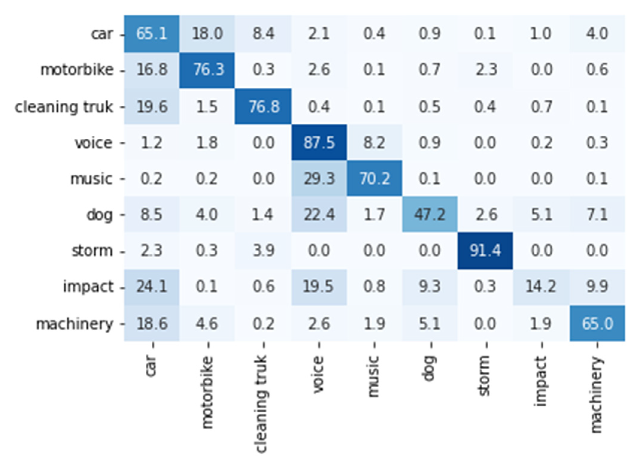
Finally, in Figure 6, we present the overall confusion matrix at fragment level for the best system, i.e., the AST architecture. The rows of the matrix represent the true labels while the columns show the predictions. Darker colors represent the highest scores. It can be said that the system classifies well the “Storm”, “Voice”, “Cleaning-truck” and “Motorbike” categories. On the contrary, the “Impact” category presents the worst classification rate with 14.2% of correct answers. Among the categories belonging to the traffic group (car, motorbike and cleaning truck), it is observed that the fragments that have not been correctly classified are confused with the other categories of the same group. “Voice” and “Music” categories are also mixed to some extent. This is probably due to the fact that many of the occurrences of music are sung songs.

5.3. Semi-Supervised Strategy for Automatic Labelling

As we have mentioned before, one of the issues of obtaining datasets to train urban-sound-event classifying systems is the initial labelling of the sound events that are registered by the monitoring devices. In this work, for the supervised part (SD) of the database, we used the 72 dB(A) threshold to obtain a manageable set of clips that could be labelled manually. However, we wanted to tackle the problem of automating the labelling for larger datasets. With this objective, a new set of events, with SPLs between 71 and 72 dB(A)s, was extracted from the recordings and manually labelled. This dataset was used to experiment with unsupervised training and, thus, was called the unsupervised dataset (UD). We presented a novel semi-supervised strategy to train a classifier for automatic labelling. Such a strategy can be applied to create the final classifier directly, but also as a way of obtaining an initial labelling that can be refined by human labellers afterwards. In order to evaluate the proposed strategy, we carried out an experiment using the convolutional architectures.

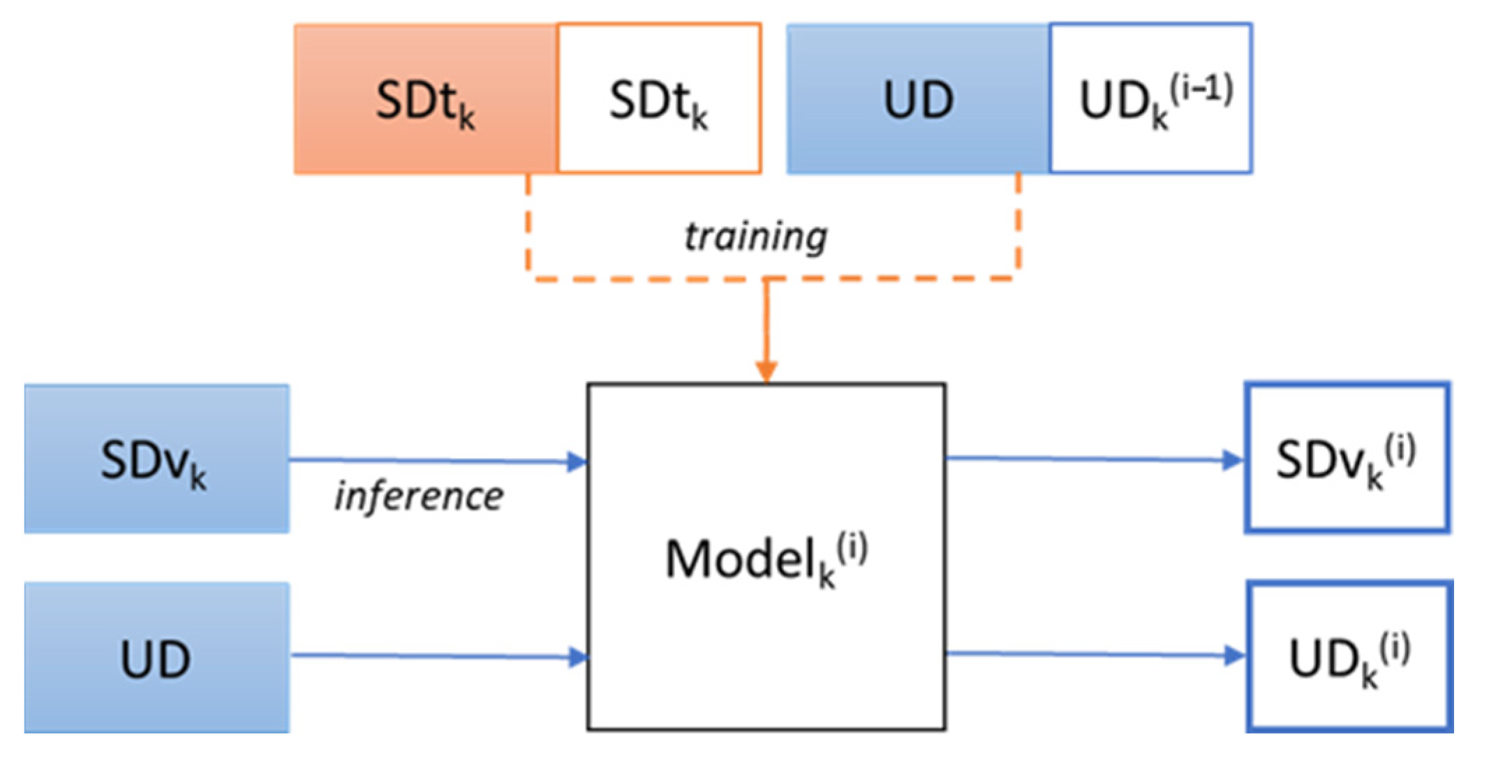
The proposed semi-supervised training method consists of several training and labelling iterations using labelled data (SD part) and unlabelled one (UD part). In the process the unlabelled data is automatically labelled and the accuracy of this labelling is refined iteratively. We have applied cross-validation for the evaluation of the method and thus the semi-supervised training iterative process that we describe bellow have been repeated 5 times using different folds of the SD part as train and validation data. The process is depicted in Figure 7.

For a particular cross-validation iteration (k), we reserve one of the folds of the SD part of the dataset for validation SDv_k and the rest 4 folders are the labelled part for training (SDt_k). On the first iteration of the semi-supervised labelling process (iter0 or i = 0), we train the system using the labelled part, SDt_k. UD_k⁽⁻¹⁾ is not used in this initial training because it has no labels, i.e., UD_k⁽⁻¹⁾ is empty. Once the training is finished, we obtain the labels for two different groups of data. The first group is the unlabelled part (getting the predicted labels UD_k⁽⁰⁾), and the second one is the reserved validation fold of SDv_k data, getting the corresponding SDv_k⁽⁰⁾ labels. In the second iteration (i = 1), the model is trained again but in this case the UD dataset with the new labels automatically predicted in the previous iteration UD_k⁽⁰⁾, is added to the initial training set (the SDt_k part). The resulting model, Model_k⁽¹⁾ is used to relabel the UD getting UD_k⁽¹⁾ and the validation SDv_k, getting a new set of labels, SDv_k⁽¹⁾. We repeat the process for four more iterations and analyse the recall of the labelling obtained in each iteration for the UD part, for the SDv_k part and the combination of both (SDv_k&UD) in order to see the overall effect in the classification performance. The idea is to check if the system is able to improve using its own predictions of the unsupervised data in a self-convergence iteration sequence. As we have mentioned before, in the following experiments this process has been performed 5 times using 4 different folds to compose the training dataset SDt_k and the remaining fold as validation dataset SDv_k. The UD part is used entirely in every cross-validation iteration, without dividing it in folds. We have decided to do so because its labelling ground truth information is never used in the training process, and because the amount of samples of this part was not very big. Note that although the UD audios are the same for each of the k folds of the cross-validation, the labels predicted are different because the training material for the Model_k has been different, that is why it is denoted by the subscript k in UD_k⁽ⁱ⁾.

5.3.1. Results for Four-Class Taxonomy

Table 7. Recall results (mean and standard deviation) in the semi-supervised experiment at the fragment level, coarse classes. Data in %.

ConvBlock				ResNet
Iterations	UD (m ± σ)	SDv (m ± σ)	SDv&UD (m ± σ)	UD (m ± σ)	SDv (m ± σ)	SDv&UD (m ± σ)
Iter0	66.6 ± 3.3	82.4 ± 5.7	75.5 ± 2.5	68.6 ± 1.9	82.9 ± 5.0	77.0 ± 2.2
Iter1	67.6 ± 2.8	82.2 ± 6.5	76.0 ± 3.1	69.0 ± 3.3	83.0 ± 4.5	77.3 ± 2.6
Iter2	68.2 ± 1.8	82.2 ± 5.6	76.7 ± 1.9	70.3 ± 2.9	81.8 ± 5.8	77.6 ± 2.7
Iter3	68.4 ± 3.4	82.3 ± 5.6	76.8 ± 2.6	69.8 ± 3.1	82.4 ± 3.5	77.4 ± 2.4
Iter4	69.4 ± 2.2	82.8 ± 4.4	77.5 ± 1.5	69.7 ± 2.9	82.4 ± 4.8	77.4 ± 2.0

shows how the macro-average recall evolves with each iteration of the method for each dataset. This value is actually the mean recall averaged for the k = 5 cross-validation iterations.

The results show an improvement in both data sets and in both classifiers. If we look to the ConvBlock results, the UD part improved by 2.8 points and the SDv&UD part by 2 points. It has to be noticed that this improvement did not impair the classification of the SD part, which indeed improved by 0.4. If we take a look at the ResNet results, the UD part was the one that improved most, by 1.7 points, followed by the SDv&UD part, which only improved 0.6 points. In this case, this improvement was achieved at the expense of a slight reduction (0.5 points) in the SDv part.

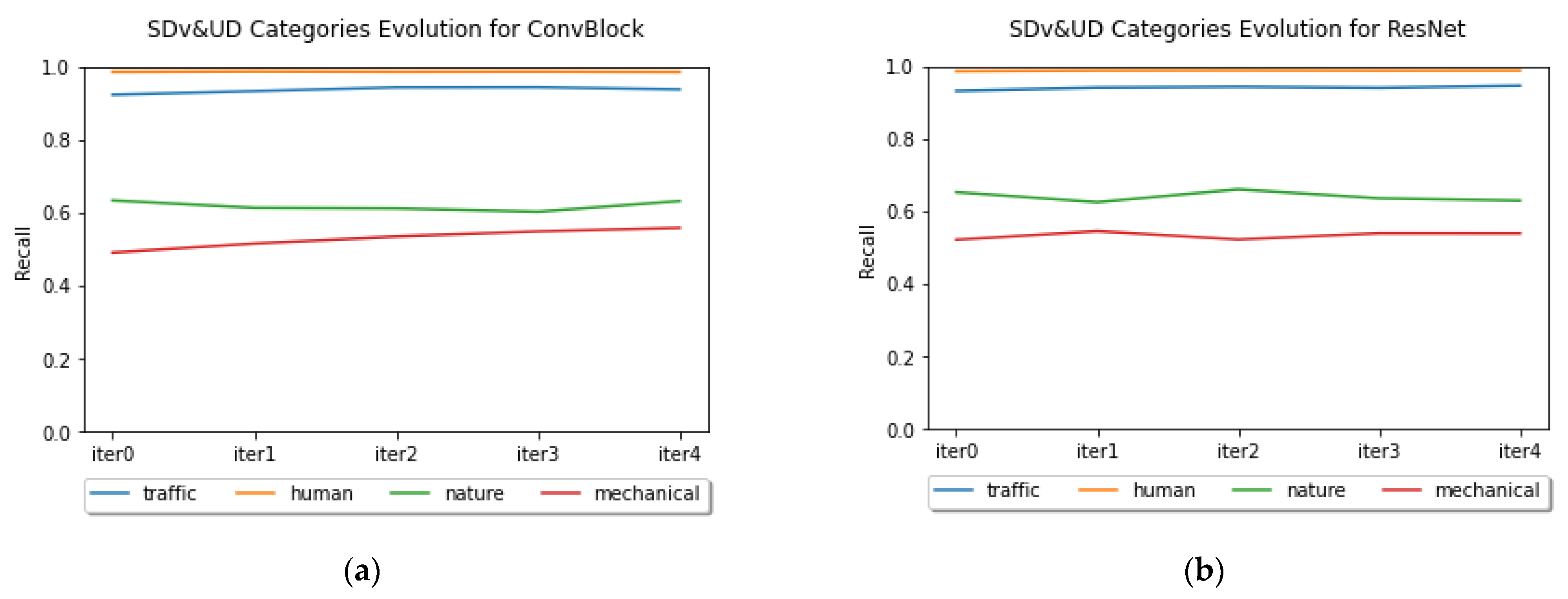
In Figure 8, we can see the evolution of the recall values of the four categories through the different iterations, considering the whole datasets (SDv&UD). The best performing classes had slight improvements during the process while the worse ones behaved irregularly.

5.3.2. Results for Nine-Class Taxonomy

Table 8. Recall results (mean and standard deviation) of the semi-supervised experiment at fragment-level fine classes. Data in %.

ConvBlock				ResNet
Iterations	UD (m ± σ)	SDv (m ± σ)	SDv&UD (m ± σ)	UD (m ± σ)	SDv (m ± σ)	SDv&UD (m ± σ)
iter0	56.5 ± 4.2	64.7 ± 4.3	59.2 ± 2.0	56.3 ± 1.8	64.4 ± 5.1	58.9 ± 3.2
iter1	61.2 ± 1.3	63.0 ± 2.7	60.5 ± 1.2	59.8 ± 1.5	64.5 ± 2.8	59.8 ± 2.1
iter2	61.3 ± 1.3	62.5 ± 2.5	60.1 ± 2.0	59.8 ± 1.8	62.2 ± 2.4	59.2 ± 1.7
iter3	62.6 ± 1.0	62.9 ± 3.5	61.0 ± 2.1	60.4 ± 2.7	62.3 ± 3.0	59.7 ± 2.5
iter4	62.7 ± 4.8	62.1 ± 5.2	61.0 ± 1.8	60.2 ± 1.7	60.2 ± 3.7	58.6 ± 1.5

shows the recall results of each of the iterations for each of the datasets. We calculated the metrics as described in Section 5.3.1.

For the ConvBlock system, an improvement was observed up to iter4 for the UD part and up to iter 3 for the SDv&UD part. In the case of the ResNet, an improvement was observed up to iter3 for the UD part and up to iter2 for the SDv&UD part.

The improvement rate is different for both system. For the ConvBlock system, the UD part improves 6.2 points and the SDv&UD improves 1.8 points. While, for the ResNet the UD part improves 4.1 and the SDv&UD part improves nearly 1 point. The SDv part only improves in the first iteration and then loses recall. The improvement in the UD part compensates the loss of accuracy of the SDv part on the SDv&UD result.

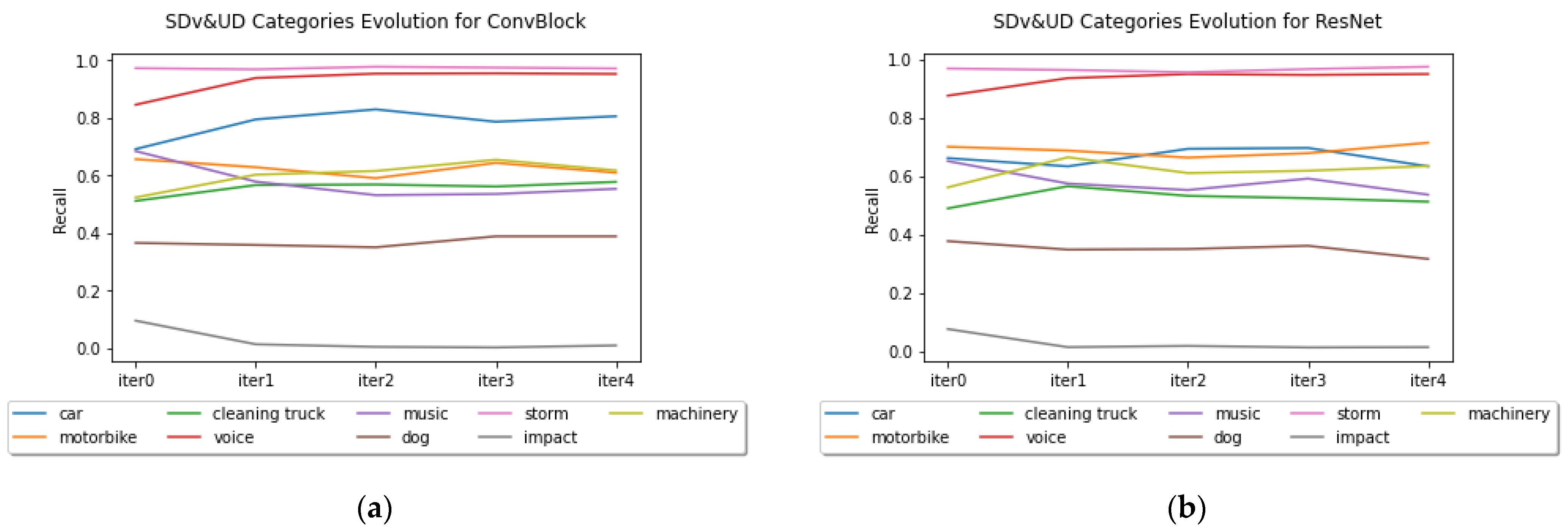
Figure 9 shows the evolution of the recall results for the different categories during the different iterations for both architectures. We present the results for the SDv&UD dataset. In both cases it can be seen that the good performing classes tend to improve with the through the iteration whereas the worse performing class “Impact” degrades. The classes with intermediate recalls vary in an unpredictable way.

6. Conclusions

In this paper, we described a new sound-classification database, NoisenseDB. The database was recorded in an urban environment and high-SPL events were extracted and labelled by a single supervisor following a two-level taxonomy. The database is publicly available for research upon request.

The database was used to evaluate and obtain baseline results for three different types of neural network-based architectures, two of them developed expressly for this work, and the third a state-of-the-art system (AST). Data-augmentation and transfer learning techniques were applied in these systems. We tested the three architectures for the defined taxonomy, both for the coarse and fine categories.

The results of the evaluation using the coarse level of the taxonomy (4 categories) gave an overall performance around 82% for fragment level classification and 70% for entire sound clip classification, with the two original neural architectures proposed by the authors performing at the same level as the AST. For the fine level of the taxonomy, the results are around 64% for all the systems.

The classifiers tended to confuse the categories belonging to the traffic group (“Car”, “Motorbike” and “Cleaning truck”) and also “Voice” and “Music”. The databases were very unbalanced and the categories with few samples (“Impact”, “Dog”) were very hard to classify.

Trying to tackle the problem of the human labelling of the large amounts of audio produced by a continuous monitoring system, we explored the possibility of a semi-supervised procedure. This experiment has shown that the initial labelling of part of the database can be used to effectively label other audio segments, and that this automated labelled part can be used to retrain the system for two or more iterations so as the automated labelling is refined. Including this new material in the training iterations does not impair the performance of the system. Actually, it can slightly improve the overall performance of the system in the first iterations.

The proposed semi-supervised labelling procedure can be used to obtain new automatically labelled data that can be used for the refinement of the models in continuous training applications. These preliminary experiments will be enhanced with more data to better understand the behaviour of the procedure.

References

1. Directive 2002/49/EC of the European Parliament and of the Council of 25 June 2002 Relating to the Assessment and Management of Environmental Noise—Declaration by the Commission in the Conciliation Committee on the Directive Relating to the Assessment and Management of Environmental Noise. Official Journal L 189, 18/07/2002 P. 0012–0026. Available online: https://eur-lex.europa.eu/eli/dir/2002/49/oj (accessed on 5 May 2019).
2. European Environment Agency. Environmental Noise in Europe—2020. EEA Report No. 22/2019. Available online: https://www.eea.europa.eu/publications/environmental-noise-in-europe (accessed on 5 March 2020).
3. Homar Santaner, V.; Ruíz Pérez, M.; Alorda Ladaria, B. Informe Técnico Para la Implantación y Explotación de la red de Sensores. SmartSensPORT-PALMA. Available online: https://www.portsdebalears.com/sites/default/files/REDsensPORTPALMAp.pdf (accessed on 5 May 2019).
4. Wang, W. (Ed.) Preface of Machine Audition Principles, Algorithms and Systems; IGI Global: Guildford, UK, 2011. [Google Scholar] [CrossRef]
5. Mesaros, A.; Heittola, T.; Virtanen, T.; Plumbley, M.D. Sound event detection: A tutorial. IEEE Signal Process. Mag. 2021, 38, 67–83. [Google Scholar] [CrossRef]
6. Piczak, K.J. Environmental sound classification with convolutional neural networks. In Proceedings of the IEEE 25th International Workshop on Machine Learning for Signal Processing (MLSP), Boston, MA, USA, 17–20 September 2015. [Google Scholar] [CrossRef]
7. Incze, Á.; Jancsó, H.B.; Szilagyi, Z.; Farkas, A.; Sulyok, C. Bird sound recognition using a convolutional neural network. In Proceedings of the IEEE 16th International Symposium on Intelligent Systems and Informatics, Subotica, Serbia, 13–15 September 2018; pp. 295–300. [Google Scholar] [CrossRef]
8. Mehyadin, A.E.; Abdulazeez, A.M.; Hasan, D.A.; Saeed, J.N. Birds sound classification based on machine learning algorithms. Asian J. Res. Comput. Sci. 2021, 9, 1–11. [Google Scholar] [CrossRef]
9. Bello, J.P.; Silva, C.; Nov, O.; Luke Dubois, R.; Arora, A.; Salamon, J.; Doraiswamy, H. SonyC: A System for monitoring, analyzing, and mitigating urban noise pollution. Commun. ACM 2019, 62, 68–77. [Google Scholar] [CrossRef]
10. Tsalera, E.; Papadakis, A.; Samarakou, M. Monitoring, profiling and classification of urban environmental noise using sound characteristics and the KNN algorithm. Energy Rep. 2020, 6, 223–230. [Google Scholar] [CrossRef]
11. Shah, S.K.; Tariq, Z.; Lee, Y. IoT based Urban Noise Monitoring in Deep Learning using Historical Reports. In Proceedings of the IEEE International Conference on Big Data, Los Angeles, CA, USA, 9–12 December 2019; pp. 4179–4184. [Google Scholar] [CrossRef]
12. Wang, S.; Mesaros, A.; Heittola, T.; Virtanen, T. A curated dataset of urban scenes for audio -visual scene analysis. In Proceedings of the ICASSP 2021 IEEE International Conference on Acoustics, Speech and Signal Processing (ICASSP), Toronto, ON, Canada, 6–11 June 2021; pp. 626–630. [Google Scholar] [CrossRef]
13. Cartwright, M.; Elisa, A.; Mendez, M.; Cramer, J.; Lostanlen, V.; Dove, G.; Bello, J.P. SONYC Urban Sound Tagging (SONYC-UST): A multilabel dataset from an urban acoustic sensor network. In Proceedings of the Detection and Classification of Acoustics Scenes and Events Workshop, New York, NY, USA, 25–26 October 2019; pp. 35–39. Available online: https://dcase.community/documents/workshop2019/proceedings/DCASE2019Workshop_Cartwright_4.pdf (accessed on 10 January 2020).
14. Martín-Morató, I.; Paissan, F.; Ancilotto, A.; Heittola, T.; Mesaros, A.; Farella, E.; Virtanen, T. Low-Complexity Acoustic Scene Classification in DCASE 2022 Challenge. In Proceedings of the Detection and Classification of Acoustics Scenes and Events Workshop, Nantes, France, 3–4 November 2022; pp. 3–7. Available online: https://dcase.community/documents/workshop2022/proceedings/DCASE2022Workshop_Martin-Morato_32.pdf (accessed on 8 November 2022).
15. Cai, Y.; Tang, H.; Zhu, C.; Li, S.; Shao, X. DCASE 2022 Submission: Low-Complexity Model Based on Depthwise Separable CNN for Acoustic Scene Classification. Technical Report in the Detection and Classification of Acoustic Scenes and Events Challenge (DCASE). 2022. Available online: https://dcase.community/documents/challenge2022/technical_reports/DCASE2022_Cai_111_t1.pdf (accessed on 20 July 2022).
16. Tsalera, E.; Papadakis, A.; Samarakou, M. Comparison of Pre-Trained CNNs for Audio Classification Using Transfer Learning. J. Sens. Actuator Netw. 2021, 10, 72. [Google Scholar] [CrossRef]
17. Arnault, A.; Riche, N. CRNNs for Urban Sound Tagging with Spatiotemporal Context. Technical Report in the Detection and Classification of Acoustic Scenes and Events Challenge (DCASE). 2020. Available online: https://dcase.community/documents/challenge2020/technical_reports/DCASE2020_Arnault_70_t5.pdf (accessed on 16 July 2020).
18. Bahmei, B.; Birmingham, E.; Arzanpour, S. CNN-RNN and data augmentation using deep convolutional generative adversarial network for environmental sound classification. IEEE Signal Process. Lett. 2022, 29, 682–686. [Google Scholar] [CrossRef]
19. Bai, J.; Chen, C.; Wang, M.; Chen, J.; Zhang, X.; Yan, Q. Data Augmentation Based System for Urban Sound Tagging. Technical Report in the Detection and Classification of Acoustic Scenes and Events Challenge (DCASE) 2020. Available online: https://dcase.community/documents/challenge2020/technical_reports/DCASE2020_Bai_127_t5.pdf (accessed on 16 July 2020).
20. Liang, J.; Zeng, C.; Shi, C.; Zhang, L.; Zhou, Y.; Li, Y.; Zhou, Y.; Tan, T. Low-Complexity Acoustic Scene Classification Based on Residual Net. Technical Report in the Detection and Classification of Acoustic Scenes and Events Challenge (DCASE). 2022. Available online: https://dcase.community/documents/challenge2022/technical_reports/DCASE2022_Liang_64_t1.pdf (accessed on 16 July 2022).
21. He, K.; Zhang, X.; Ren, S.; Sun, J. Deep residual learning for image recognition. In Proceedings of the IEEE Computer Society Conference on Computer Vision and Pattern Recognition, Las Vegas, NV, USA, 27–30 June 2016; pp. 770–778. [Google Scholar] [CrossRef]
22. Palanisamy, K.; Singhania, D.; Yao, A. Rethinking CNN models for audio classification. arXiv 2020, arXiv:2007.11154. [Google Scholar]
23. Gong, Y.; Chung, Y.-A.; Glass, J. AST: Audio Spectrogram Transformer. In Proceedings of the Annual Conference of the International Speech Communication Association, ISCA, Brno, Czchec Republic, 30 August–3 September 2021. [Google Scholar] [CrossRef]
24. Koutini, K.; Schl, J.; Eghbal-zadeh, H.; Widmer, G. Efficient training of audio transformers with patchout. In Proceedings of the 23rd Annual Conference of the International Speech Communication Association, Interspeech, Incheon, Republic of Korea, 18–22 September 2022. [Google Scholar] [CrossRef]
25. Sooyoung, P.; Youngho, J.; Taejin, L. Many-to-many audio spectrogram transformer: Transformer for sound event localization and detection. In Proceedings of the Detection and Classification of Acoustics Scenes Workshop (DCASE), Online, 15–19 November 2021. [Google Scholar]
26. Zhang, Z.; Xu, S.; Zhang, S.; Qiao, T.; Cao, S. Attention based convolutional recurrent neural network for environmental sound classification. Neurocomputing 2020, 453, 896–903. [Google Scholar] [CrossRef]
27. Tripathi, A.M.; Mishra, A. Environment sound classification using an attention-based residual neural network. Neurocomputing 2021, 460, 409–423. [Google Scholar] [CrossRef]
28. Hou, Y.; Tan, Y.; Chang, Y.; Huang, T.; Li, S.; Shao, X.; Botteldooren, D. CNN-Based Dual-Stream Network for Audio-Visual Scene Classification. Technical Report in the Detection and Classification of Acoustic Scenes Challenge 2021. Available online: https://dcase.community/documents/challenge2021/technical_reports/DCASE2021_Hou_89_t1.pdf (accessed on 21 July 2021).
29. Wang, Q.; Zheng, S.; Li, Y.; Wang, Y.; Wu, Y.; Hu, H. A Model Ensemble Approach for Audio-Visual Scene Classification. Technical Report in the Detection and Classification of Acoustic Scenes and Events Challenge (DCASE) 2021. Available online: https://dcase.community/documents/challenge2021/technical_reports/DCASE2021_Du_124_t1.pdf (accessed on 21 July 2021).
30. Liu, Z.; Fang, J.; Hong, X.; Liu, G. Multisystem Fusion Model Based on Tag Relationship. Technical Report in the Detection and Classification of Acoustic Scenes and Events Challenge (DCASE) 2020. Available online: https://dcase.community/documents/challenge2020/technical_reports/DCASE2020_Liu_54_t5.pdf (accessed on 16 July 2020).
31. Wang, M.; Chen, C.; Xie, Y.; Chen, H.; Liu, Y.; Zhang, P. Audio-Visual Scene Classification Using Transfer Learning and Hybrid Fusion Strategy. Technical Report in Detection and Classification of Acoustic Scenes and Events Challenge (DCASE) 2021. Available online: https://dcase.community/documents/challenge2021/technical_reports/DCASE2021_Zhang_109 (accessed on 21 July 2021).
32. Xu, L.; Wang, J.; Wang, L.; Bi, S.; Zhang, J.; Ma, Q. Human Sound Classification based on Feature Fusion Method with Air and Bone Conducted Signal. In Proceedings of the 23rd Annual Conference of the International Speech Communication Association (Interspeech), Incheon, Republic of Korea, 18–20 September 2022; pp. 1506–1510. [Google Scholar]
33. Fedorishin, D.; Sankaran, N.; Mohan, D.; Birgiolas, J.; Schneider, P.; Setlur, S.; Govindaraju, V. Investigating Waveform Spectrogram Feature Fusion for Acoustic Scene Classification. Technical Report in the Detection and Classification of Acoustic Scenes and Events Challenge 2021 (DCASE). Available online: https://dcase.community/documents/challenge2021/technical_reports/DCASE2021_Fedorishin_97_t1.pdf (accessed on 21 July 2021).
34. Piczak, K.J. ESC: Dataset for environmental sound classification. In Proceedings of the 23rd ACM International Conference on Multimedia (MM ′15), Brisbane, Australia, 26–30 October 2015; Association for Computing Machinery: New York, NY, USA, 2015; pp. 1015–1018. [Google Scholar] [CrossRef]
35. Salamon, J.; Jacoby, C.; Bello, J.P. A dataset and taxonomy for urban sound research. In Proceedings of the 22nd ACM International Conference on Multimedia, Orlando, FL, USA, 3–7 November 2014; pp. 1041–1044. [Google Scholar] [CrossRef]
36. Gemmeke, J.F.; Ellis, D.P.; Freedman, D.; Jansen, A.; Lawrence, W.; Moore, R.C.; Plakal, M.; Ritter, M. AudioSet: Antology and human-labeled dataset for audio events. In Proceedings of the International Conference on Acoustics, Speech and Signal Processing (ICASSP), New Orleans, LA, USA, 5–9 March 2017; pp. 776–780. [Google Scholar] [CrossRef]
37. Cartwright, M.; Cramer, J.; Mendez, A.E.; Wang, Y.; Wu, H.H.; Lostanlen, V.; Fuentes, M.; Dove, G.; Mydlarz, C.; Salamon, J.; et al. SONYC-UST-V2: An urban sound tagging dataset with spatiotemporal context. In Proceedings of the 5th Workshop on Detection and Classification of Acoustic Scenes and Events (DCASE 2020), Glasgow, UK, 4–9 May 2019. [Google Scholar]
38. Font, F.; Roma, G.; Serra, X. Freesound Technical Demo. In Proceedings of the 21st ACM International Conference on Multimedia, Barcelona, Spain, 21–25 October 2013. [Google Scholar] [CrossRef]
39. Ooi, K.; Watcharasupat, K.N.; Peksi, S.; Karnapi, F.; ONg, Z.T.; Chua, D.; Gan, W.S. A strongly labelled polyphonic dataset of urban sounds with spatiotemporal context. In Proceedings of the Asia-Pacific Signal and Information Processing Association Annual Summit and Conference (APSIP AASC), Tokyo, Japan, 14–17 December 2021; pp. 982–988. [Google Scholar]
40. Cartwright, M.; Dove, G.; Méndez, A.E.M.; Bello, J.P.; Nov, O. Crowdsourcing multi-label audio annotation tasks with citizen Scientists. In Proceedings of the 2019 CHI Conference on Human Factors in Computing Systems, Glasgow, UK, 4–9 May 2019. [Google Scholar] [CrossRef]
41. Hantke, S.; Abstreiter, A.; Cummins, N.; Schuller, B. Trustability-Based dynamic active learning for crowdsourced labelling of emotional audio data. IEEE Access 2018, 6, 42142–42155. [Google Scholar] [CrossRef]
42. Gururani, S.; Lerch, A. Semi-Supervised audio classification with partially labeled data. In Proceedings of the 23rd IEEE International Symposium on Multimedia (ISM), Naple, Italy, 29 November–1 December 2021. [Google Scholar] [CrossRef]
43. Lee, D.-H. Pseudo-label: The simple and efficient semi-supervised learning method for deep neural networks. In Proceedings of the International Conference of Machine Learning (ICML), Atlanta, GA, USA, 16–21 June 2013; Available online: https://www.researchgate.net/publication/280581078_Pseudo-Label_The_Simple_and_Efficient_Semi-Supervised_Learning_Method_for_Deep_Neural_Networks (accessed on 1 November 2021).
44. Amini, M.; Feofanov, V.; Pauletto, L.; Devijver, E.; Maximov, Y. Self-Training A Survey. arXiv. Available online: http://arxiv.org/abs/2202.12040 (accessed on 15 February 2023).
45. Cramer, J.; Wu, H.H.; Salamon, J.; Bello, J.P. Look, Listen, and Learn More: Design choices for deep audio embeddings. In Proceedings of the IEEE International Conference on Acoustics, Speech and Signal (ICASSP), Brighton, UK, 12–17 May 2019. [Google Scholar] [CrossRef]
46. McFee, B.; Raffel, C.; Liang, D.; Ellis, D.; McVicar, M.; Battenberg, E.; Nieto, O. Librosa: Audio and music signal analysis in python. In Proceedings of the 14th Python in Science Conference, Austin, TX, USA, 6–12 July 2014; Volume 8, pp. 18–25. [Google Scholar] [CrossRef]
47. Zhang, H.; Cisse, M.; Dauphin, Y.N.; Lopez-Paz, D. MixUp: Beyond Empirical Risk Minimization. In Proceedings of the 6th International Conference on Learning Representations, ICLR, Vancouver, BC, Canada, 30 April–3 May 2018. [Google Scholar]
48. Dwivedi, P. Deep Learning-Resnet Keras. Github. Available online: https://github.com/priya-dwivedi/Deep-learning/blob/master/resnet_keras/ResidualNetworks_yourself.ipynb (accessed on 4 January 2019).
49. Touvron, H.; Cord, M.; Douze, M.; Massa, F.; Sablayrolles, A.; Jégou, H.; Ai, F. Training data-efficient image transformers distillation through attention. In Proceedings of the 38th International Conference on Machine Learning, PMLR, Online, 18–24 July 2021; pp. 10347–10357. Available online: https://proceedings.mlr.press/v139/touvron21a.html (accessed on 13 November 2021).
50. Deng, J.; Dong, W.; Socher, R.; Li, L.-J.; Li, K.; Li, F.-F. ImageNet: A large-scale hierarchical image database. In Proceedings of the IEEE Conference on Computer Vision and Pattern Recognition, Miami, FL, USA, 20–25 June 2009; pp. 248–255. [Google Scholar] [CrossRef]
51. Gong, Y. AST: Audio Spectrogram Transformer. Github. Available online: https://github.com/YuanGongND/ast (accessed on 15 May 2021).
52. Vaswani, A.; Shazeer, N.; Parmar, N.; Uszkoreit, J.; Jones, L.; Gómez, A.N.; Kaiser, L.; Polosukhin, I. Attention is all you need. In Proceedings of the 1st Conference on Advances in Neural Information Processing Systems (NIPS), Long Beach, CA, USA, 4–9 December 2017; Available online: https://papers.nips.cc/paper_files/paper/2017/file/3f5ee243547dee91fbd053c1c4a845aa-Paper.pdf (accessed on 15 May 2021).
53. Sokolova, M.; Lapalme, G. A systematic analysis of performance measures for classification tasks. Inf. Process. Manag. 2009, 45, 427–437. [Google Scholar] [CrossRef]
Figure 1. Noise-monitoring device.
Applsci 13 09358 g001
Figure 2. Developed architectures, (a) Sound event classification system based on ConvBlock, and (b) sound event classification system based on ResNet.
Applsci 13 09358 g002
Figure 3. Convolutional block.
Applsci 13 09358 g003
Figure 4. A CBIB block of the ResNet showing the Convolutional block (CB), and the Identity Block (IB).
Applsci 13 09358 g004
Figure 5. Overall confusion matrix for ResNet at the fragment level. Data in %.
Applsci 13 09358 g005
Figure 6. Overall confusion matrix for the AST at the fragment level. Data in %.
Applsci 13 09358 g006
Figure 7. Diagram representing the i-th iteration of the semi-supervised labelling process for the k-th cross-validation fold. Filled boxes represent the audio of the datasets and unfilled boxes represent the labels.
Applsci 13 09358 g007
Figure 8. Evolution of recall results by category for the SDv&UD data: (a) ConvBlock, and (b) ResNet.
Applsci 13 09358 g008
Figure 9. SDv&UD category evolution: (a) ConvBlock, and (b) ResNet.
Applsci 13 09358 g009