Enhancing Lane-Tracking Performance in Challenging Driving Environments through Parameter Optimization and a Restriction System

Abstract

The autonomous driving market has experienced rapid growth in recent times. From systems that assist drivers in keeping within their lanes to systems that recognize obstacles using sensors and then handle those obstacles, there are various types of systems in autonomous driving. The sensors used in autonomous driving systems include infrared detection devices, lidar, ultrasonic sensors, and cameras. Among these sensors, cameras are widely used. This paper proposes a method for stable lane detection from images captured by camera sensors in diverse environments. First, the system utilizes a bilateral filter and multiscale retinex (MSR) with experimentally optimized set parameters to suppress image noise while increasing contrast. Subsequently, the Canny edge detector is employed to detect the edges of the lane candidates, followed by utilizing the Hough transform to make straight lines from the land candidate images. Then, using a proposed restriction system, only the two lines that the current vehicle is actively driving within are detected from the candidate lines. Furthermore, the lane position information from the previous frame is combined with the lane information from the current frame to correct the current lane position. The Kalman filter is then used to predict the lane position in the next frame. The proposed lane-detection method was evaluated in various scenarios, including rainy conditions, low-light nighttime environments with minimal street lighting, scenarios with interfering guidelines within the lane area, and scenarios with significant noise caused by water droplets on the camera. Both qualitative and quantitative experimental results demonstrate that the lane-detection method presented in this paper effectively suppresses noise and accurately detects the two active lanes during driving.

1. Introduction

Recently, extensive research has been conducted on autonomous driving systems, which encompass a variety of types. For instance, the lane-change assist system utilizes cameras for improved visibility, while the lane-departure warning system detects the changes and alerts the driver, employing audible signals and steering wheel correction when there is a risk of departing from the lane while driving. Furthermore, the lane-keeping assist system (LKAS) helps maintain the vehicle within the lane during operation. Effectively to assist the driver, these systems rely on accurate lane detection and identification to determine the shape and position of the lanes.

Advanced driver-assistance systems technologies employ a range of sensors, including cameras, ultrasonic sensors, and radars. Among these, cameras offer a cost-effective solution while providing a substantial amount of information. Additionally, when combined with ultrasonic or radar sensors, cameras can serve as auxiliary sensors. Consequently, cameras are extensively utilized in these systems. Lane detection from camera-captured images can be achieved through two methods: the model-based method, which utilizes mathematical models to detect and predict lane structures, and the feature-based method, which identifies lanes by analyzing pixel information such as patterns, colors, or gradients. However, the emergence and widespread use of deep learning methods employing neural networks has led to an increasing adoption of such techniques for lane detection across various domains. Accordingly, this paper classifies the pre-deep learning methods as tool-based methods, while methods employing neural networks are referred to as deep learning methods, and appropriate explanations are provided accordingly.

One prominent method in the tool-based approach involves leveraging lane edges. This method utilizes Canny edge detection to identify edges, followed by the application of the Hough transform on the resulting edge image to detect straight lines. Another approach involves utilizing random sample consensus (RANSAC) to eliminate outliers or employing density-based spatial clustering of application with noise (DBSCAN) for clustering on the edge image. Another avenue is the utilization of color for lane detection. Several methods employ the RGB color space or employ color segmentation in color space models such as HSV and Lab to differentiate pixels and classify them into respective classes. The previously discussed methods primarily focus on lane detection and information about other vehicles during driving. However, for autonomous driving, a comprehensive approach is required, which encompasses not only lanes and other vehicles but also road network topology, signal locations, signage, and buildings. A digital map system called high-definition map (HD map) contains such detailed road information. HD maps are created based on various sensor data, including cameras, lidar, and GPS. On the other hand, in the deep learning-based approach, the U-Net ConvLSTM, a variation of U-Net with skip connections, can be employed for pixel-level segmentation. Additionally, some methods utilize generative adversarial network (GAN) models to generate lane-detection images based on input frames.

As the interest in autonomous driving systems continues to increase, numerous companies and countries are actively conducting research and pursuing commercialization in this field. Given the variations in geography, laws, and regulations, road and natural environments differ across different countries. Consequently, autonomous driving systems must adapt and operate reliably in diverse environments. This paper presents a method for robust lane detection in challenging environments where lane detection using cameras becomes difficult. The proposed method involves several steps. First, the brightness of the input image is analyzed to differentiate between day and night conditions. Next, noise is suppressed, and contrast is optimized using carefully tuned parameters specific to each time period. The Canny edge detector is then employed to detect lane candidates, and the Hough transform is utilized to identify all lines present in the resulting lane-candidate image. Subsequently, the proposed restriction system is employed to identify the two lines with the highest probability of being lane lines. Finally, the positions of these two lines are estimated and updated using the Kalman filter, enabling the final detection of the lane lines.

2. Related Works

2.1. Tone Correction

Tone correction is a widely employed method for adapting the brightness of an image to make it suitable for lane detection, achieved by adjusting the tone of the image [1,2]. Several approaches can be used to adjust the tone, including increasing the intensity value of each pixel to brighten the image or stretching the dynamic range by creating a histogram of the intensity values of all pixels in the image. Numerous techniques for tone control are available, and the selection of a specific method depends on the unique characteristics of the image and the requirements of the lane-detection algorithm.

Human vision is sensitive to the ratio of ambient brightness, which refers to the light reflected by the surrounding environment rather than the actual brightness emitted by a light source. To account for these characteristics, techniques such as histogram stretching and histogram equalization are employed to enhance the input image. Histogram stretching is a method that linearly expands the narrow dynamic range of the original image’s histogram. On the other hand, histogram equalization utilizes the cumulative density function to achieve a uniform distribution across the entire image area [3]. The distinction between these two methods can be observed in Figure 1. However, it is important to note that these tone correction methods have limited effectiveness when the image contains both dark and bright areas simultaneously. In environments where lanes are illuminated by headlights in darkness, these tone correction methods may not be suitable for improving image quality.

The single-scale retinex method is employed to enhance the contrast or sharpness of an image by eliminating background components present in the input image [4]. This is achieved by applying a Gaussian filter of a single scale to remove the background component. However, instead of using a single-scale Gaussian filter, the background component can be effectively eliminated by employing a Gaussian filter with multiple scales. This approach, known as the multiscale retinex (MSR) algorithm, generates an output image by assigning appropriate weights to the filtered results [5].

2.2. Lane Detection

2.2.1. Tool-Based Methods

Vehicle-installed cameras often exhibit poor image quality due to cost constraints and spatial environmental limitations. Consequently, the acquired images for lane detection often contain various elements that interfere with accurate detection, such as noise in low-luminance regions. To address this, a smoothing filter is applied to suppress noise and enhance edge sharpness prior to optimal edge detection. Specifically, a bilateral filter is commonly used, which reduces noise while preserving the lane edges [6]. The bilateral filter employs two parameters, intensity sigma and space sigma, which can be adjusted to control the level of edge preservation and smoothing based on the environmental information in the image.

The Canny edge detector is a powerful method for edge detection, typically involving four stages: noise reduction, edge gradient computation, nonmaximum suppression, and double thresholding and edge tracking through hysteresis [7]. These four stages can be observed in Figure 2. Although the Canny edge detector offers high detection performance, its processing speed is relatively slow due to the division into multiple stages. As a result, in cases where most lanes appear vertical in vehicle-installed cameras, an alternative approach is to utilize the faster calculation of the Sobel operator [8,9].

The Hough transform is a highly effective method for detecting approximate straight lines in edge images. It represents a straight line as a point in the domain of gradient and y-intercept. In this representation, all possible straight lines that can pass through a point are transformed into a single line in the gradient–y-intercept plane [10]. Due to this property, the Hough transform is widely utilized in lane detection. Additionally, another approach for detecting estimated lane lines in edge images involves using the RANSAC algorithm [11,12]. RANSAC is commonly employed in regression problems and consists of two steps: the hypothesis step and the verification step. The process is iterated a specified number of times set by the user. In the hypothesis step, a set of n sample data points is randomly selected from the entire dataset, and a model is predicted based on these samples. In the verification step, the number of data points that match the predicted model are counted, and the model with the maximum number of matches is saved. Through this iterative process, a lane model can be identified in the edge image, enabling lane estimation detection. Furthermore, the edge pixels in an edge image form a point cloud, and DBSCAN can be utilized to group the points based on their density in the point cloud image [13]. Several methods employ DBSCAN for lane detection in edge images [12,14]. During the density-based grouping process, there is an approach that incorporates directional information, known as directional DBSCAN (D-DBSCAN). This technique is particularly useful for detecting parking slot lines [15]. Moreover, lane detection can be performed by converting the input image into a bird’s-eye view after acquiring the camera’s internal and external parameters through camera calibration [16,17]. This method is commonly used for detecting curved lanes that are relatively distant from the camera. Autonomous driving systems not only rely on cameras but also actively involve research utilizing distance-detection sensors such as lidar. Three-dimensional lidar enables more precise distance measurements in three-dimensional space compared to lidar, but it may encounter challenges such as occlusion and out-of-range issues when reaching the sensing-range limitations of connected automated vehicles (CAV). To address these problems, HYDRO-3D combines object detection and object tracking information to infer objects, and employs a novel spatial–temporal 3D neural network to enhance the features of object detection [18]. There have been studies that contribute to the extraction, reconstruction, and evaluation of vehicle trajectories based on the cooperative perception of connected autonomous vehicles (CAV) by presenting data acquisition and analytics platforms utilizing not only cameras but also LiDAR sensors, GPS, and communication systems in autonomous driving systems [19].

The Kalman filter is a commonly employed technique for tracking lanes in successive frames after lane detection in an initial frame. It utilizes the newly obtained lane information in the current frame to correct and update the accumulated lane information from the previous frames. By leveraging this information, the Kalman filter estimates the position of the lane in the next frame [20]. Another approach for lane tracking is to utilize a particle filter [21]. This method employs a set of particles to represent the possible positions and characteristics of the continuous lanes. By iteratively updating and resampling the particles based on the observed lane information, the particle filter can track the lane across multiple frames. Furthermore, there exists a fusion method that combines both the Kalman filter and the particle filter for lane tracking [22]. This hybrid approach leverages the strengths of both filters to improve the accuracy and robustness of the lane tracking process. Kalman filters can be utilized not only for lane tracking in video but also for estimating errors in a reduced inertial navigation system (R-INS) by incorporating information from an inertial measurement unit (IMU). The IMU provides acceleration and angular rate measurements, which can be used to estimate velocity and heading errors in the R-INS. By combining these IMU measurements with velocity error measurements between R-INS and the global navigation satellite system (GNSS), a velocity-based Kalman filter can accurately estimate the errors in R-INS, including velocity and heading. This integrated approach, leveraging both visual data and GNSS measurements, enhances the accuracy of position and heading estimation in autonomous driving systems. Therefore, Kalman filters not only facilitate lane tracking but also enable the estimation of velocity and heading errors, improving the overall navigation and perception capabilities in autonomous driving systems [23,24,25].

2.2.2. Deep Learning-Based Methods

Deep learning has gained significant traction across various fields, including lane detection. Recent advancements in deep learning-based lane-detection methods can be systematically classified and presented based on different criteria. Here are two main categories:

(1)

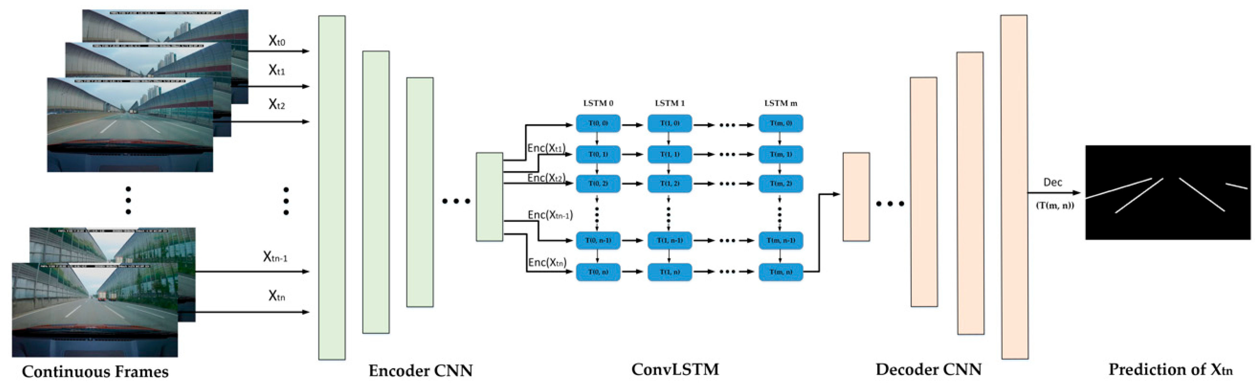
Encoder–decoder segmentation: In this approach, encoder–decoder convolutional neural networks (CNNs) are commonly used for pixelwise segmentation. SegNet is a deep fully convolutional neural network architecture specifically designed for semantic pixelwise segmentation [26,27]. LaneNet is another model that focuses on end-to-end lane detection and consists of two decoders: a segmentation branch for lane detection in a binary mask and an embedding branch for road segmentation [28]. Another variant replaces the skip connection in U-Net with a long short-term memory (LSTM) layer, shown in Figure 3 [29]. LSTM is a type of recurrent neural network (RNN) that addresses the challenge of modeling long dependencies in sequential data [30,31]. By incorporating an LSTM layer, this method effectively preserves high-dimensional information from the encoder and transmits it to the decoder. Also, there is a method to replace the standard convolution layer in the traditional U-Net with depthwise and pointwise convolutions to reduce computational complexity while maintaining the detection rate. This U-Net structure is referred to as DSUNet (depthwise and pointwise U-Net) [32].

(2)

GAN model: The GAN is composed of a generator and a discriminator [33]. Lane detection can be performed using GAN-based models [34]. One specific method proposed the embedding-loss GAN (EL-GAN) for semantic segmentation. The generator predicts lanes based on input images, while the discriminator determines the quality of the predicted lane using shared weights. This approach produces thinner lane predictions compared to regular CNN results, allowing for more accurate lane observation. It also performs well in scenarios where lanes are obscured by obstacles such as vehicles.

Figure 3. Architecture of U-Net ConvLSTM.

Figure 3. Architecture of U-Net ConvLSTM.

3. Proposed Method

The proposed lane-detection system as shown in Figure 4 consists of three stages: noise-reduction processing, lane-candidate grouping, and optimal lane detection and tracking. In the noise-reduction processing stage, techniques such as discrimination between day and night, region of interest (ROI), and a surround-dependent bilateral filter are used to reduce noise according to the input image. The lane-candidate grouping stage includes the adjusted MSR representation to optimize the tone mapping for easier lane detection. Additionally, Canny edge detection is utilized to identify edges, and the Hough transform is employed to group potential lane candidates. Finally, in the optimal lane detection and tracking stage, a restriction system is proposed to identify the actual lane within the candidate group. The Kalman filter is used to track the lane detected in the previous frame, ensuring consistent lane tracking. By following these three stages, the proposed lane-detection system aims to environment-adaptively reduce noise, group lane candidates, and accurately detect and track the optimal lane under varying driving conditions.

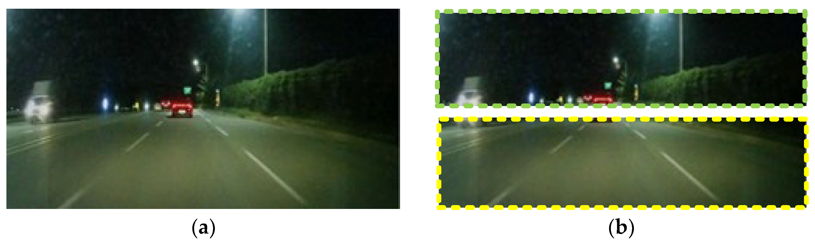
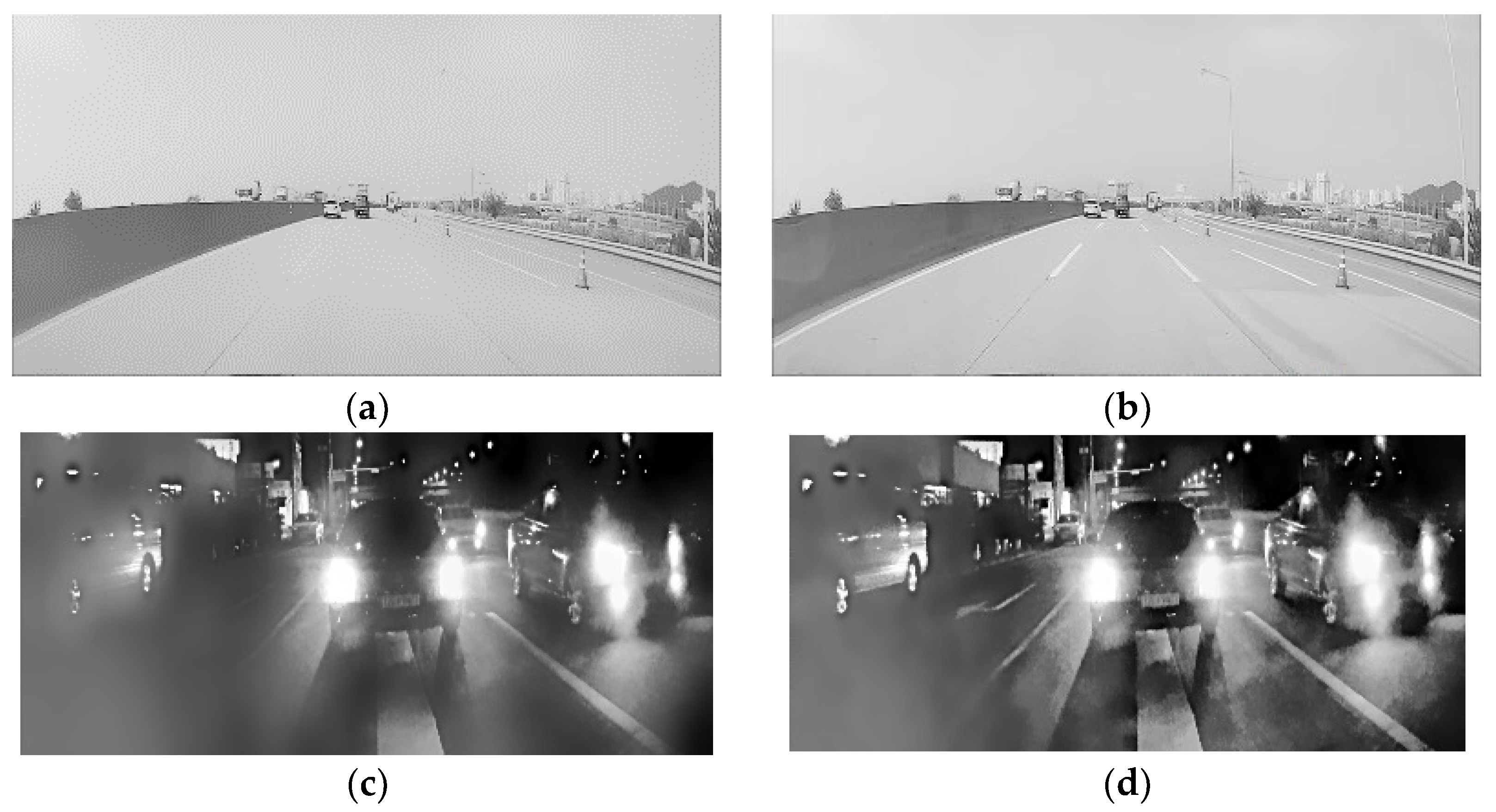
3.1. Noise-Reduction Processing

The objective of this part is to reduce noise and enhance contrast in the input image. The process begins by dividing the image into two regions: an upper region used to determine the time period of the image, and a lower region where the actual lane detection takes place. Specific parameters corresponding to the time period are applied to process the images. This differentiation between daytime and nighttime enables noise suppression and contrast enhancement tailored to each specific time period.

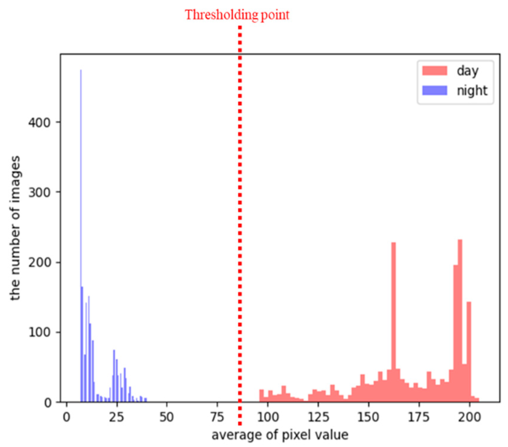
3.1.1. Discrimination between Day and Night

The input image is divided into two regions, the upper area and the lower area, known as the ROI, illustrated in Figure 5. The upper area is utilized to determine the time period of the input image, while the lower area is dedicated to lane detection.

Lane detection can be challenging due to variations in lighting conditions particular to day and to night. At night, factors such as dark surroundings, vehicle headlights, and backlights of cars ahead can hinder lane detection. During the day, lanes are generally easier to detect, but excessive sunlight can lead to blurred lane markings. Figure 6a,c demonstrate the disappearance of lanes due to inappropriate parameters, while Figure 6b,d show the benefits of using appropriate parameters for lane detection. Increasing contrast is advantageous for lane detection, especially in bright daytime conditions. However, in low-light conditions at night, the presence of oversaturated areas caused by vehicle headlights can obscure lane markings. Therefore, increasing contrast can sometimes eliminate lanes in these oversaturated regions. The parameters used in the system are specifically designed to preserve detailed edge information, which is crucial for accurate lane detection.

To distinguish between daytime and nighttime in the upper area of the image, a criterion was established based on experimentation. A total of 1800 daytime images and 1740 nighttime images were used in this experiment. The goal was to determine an appropriate threshold that can effectively differentiate between the two conditions. In order to measure brightness in the area on the road, there are numerous variables that can affect the measurement. To mitigate this, we calculated the average pixel value in the sky area of the image, as this region tends to have fewer variables. Figure 7 depicts a histogram showing the average brightness values in the sky area of each grayscale image. By cropping the sky area of the input image and calculating the average brightness, this paper determined that a value over 80 indicates a daytime condition, while a value below 80 suggests a nighttime condition. This threshold value serves as the criterion for distinguishing between day and night in the upper area of the image.

3.1.2. Suppression of Noise and Contrast Enhancement

The bilateral filter is usually used to address the concern of amplifying severe noise in the low-intensity region when applying gamma modulation for brightness improvement [6]. This part aims to environment-adaptively preserve the edge of the lane while suppressing noise before enhancing brightness. To optimize the parameters of the bilateral filter, such as the spatial sigma (${\sigma }_s$) and intensity sigma (${\sigma }_i$) in Equation (1), the line profile information in Figure 8 is utilized. By analyzing the line profile, the optimal values of ${\sigma }_s$ and ${\sigma }_i$ can be determined, ensuring a balance between noise suppression and edge preservation for accurate lane detection.

$$I^{\prime }\left(x, y\right)={{\displaystyle \sum }}_{y\in N\left(x\right)}{e}^{\frac{-\Vert y-{x\Vert }^2}{2{\sigma }_s^2}}{e}^{\frac{-\Vert I\left(y\right)-I{\left(x\right)\Vert }^2}{2{\sigma }_i^2}}I\left(x,y\right)$$

(1)

where ${\sigma }_s$ and ${\sigma }_i$ are the parameters controlling the fall-off of weights in spatial and intensity domains, respectively. $N\left(x\right)$ is a spatial neighborhood of pixel $I\left(x\right)$. ${\sigma }_s$ is the geometric spread parameter that is to be chosen based on the extent of low-pass filtering required. A large value of ${\sigma }_s$ implies a combination of values from farther distances in the image. Similarly, ${\sigma }_i$ is the parametric spread that is set to achieve the desired amount of the combination of pixel values.

This study sets the parameters of the bilateral filter according to the time of the input image. For daytime, the focus was on enhancing the edges and improving the details of the image, as the image already included sufficient illumination components due to sunlight. The images shown in Figure 9a,c have been passed through a bilateral filter with different parameters. Figure 9a is the image obtained by setting ${\sigma }_s$ and ${\sigma }_i$ to 15/255 and 2, respectively, as expressed in Equation (1). Furthermore, the image shown in Figure 9c was obtained by setting the values of ${\sigma }_s$ and ${\sigma }_i$ to 3/255 and 12, respectively. Figure 9b,d are the line profiles of the lanes in each image of Figure 9a,c, respectively. By comparing the edge gap between Figure 9c,d, the edge gap in Figure 9d is confirmed to be larger. Based on this, the parameters of the bilateral filter were set to high values for images acquired during the day.

In contrast to daytime images, nighttime images present different challenges, including the absence of sunlight and the presence of severe noise caused by headlights from other vehicles and streetlights. Therefore, the focus in nighttime image processing is on suppressing noise around the lane. In Figure 10, different bilateral filter parameters are applied to the images shown in Figure 10a,c. The images shown in Figure 10b,d represent the line profiles corresponding to Figure 10a,c respectively. By comparing the two profiles, it can be observed that the noise is effectively suppressed and the edge gaps are preserved in Figure 10b. This demonstrates the effectiveness of the chosen bilateral filter parameters in suppressing noise while maintaining edge information in nighttime images.

In this study, the MSR algorithm is adjusted to optimize the tone mapping for the enhanced lane detection in challenging harsh environments where lane identification is difficult. This processing is applied prior to the edge-detection step. Retinex image processing assumes that an image consists of a background illumination component and a reflection component. By using a Gaussian filter, the algorithm separates the illumination component from the original image and subtracts it, thus enhancing the reflection component. This can be expressed as Equation (2). To perform retinex at multiple scales, the sigma value of the Gaussian filter is varied. By selecting and combining appropriate sigma values based on the image environment, the edge components of the lanes can be effectively emphasized. Mathematically, this can be represented by Equation (3). To improve processing speed, the convolution operation of the Gaussian filter with each frame and sigma is replaced with a multiplication process in the fast Fourier transform (FFT) domain. Overall, the application of the MSR algorithm with multiple scales and the use of FFT-based processing contribute to enhancing lane edge components and improving the efficiency of lane detection in challenging dark environments.

$$SS{R}_i\left(x,y\right)=\log \left(I_i\left(x,y\right)\right)-\log \left(I_i\left(x,y\right)\ast G_{{\sigma }_i}\left(x,y\right)\right),$$

(2)

$$MSR\left(x,y\right)={{\displaystyle \sum }}_{i=1}^n{\omega }_{i}SS{R}_i\left(x,y\right),$$

(3)

where $I_i\left(x,y\right)$ is the input image, $G_{{\sigma }_i}\left(x,y\right)$ is a Gaussian filter, and ${\sigma }_i$ is the $i{ }_{th}$ sigma; convolution $I_i\left(x,y\right)$ and $G_{{\sigma }_i}(x,y$) background components can be obtained, and the background components can be subtracted from the original image.

We can obtain an image in which the reflection component is emphasized. This process is performed at multiple scales $n$ with the weight of each scale; finally, we sum them together. In this experiment, uniform weight is ensured. The lane in Figure 11 is emphasized to facilitate detection of the line profile.

In the experimental determination of the MSR parameters, the focus was on enhancing the edge gap in daytime images where there is sufficient lighting and less noise. Figure 12 illustrates the results of this experiment. The experiment involved setting each single-scale sigma value in Equation (2) to different values: 10, 90, and 200. The resulting images shown in Figure 12a,c,e were created by assigning equal weight to each ${\omega }_i$ in Equation (3), with higher weights given to lower sigma values and lower weights given to higher sigma values. By analyzing the line profiles shown in Figure 12b,d,f, it can be observed that the line profile of Figure 12f exhibits the largest edge gap. This indicates that by assigning higher weights to lower sigma values, the MSR algorithm effectively enhances the edge gap in daytime images. Through these experimental results, the optimal parameters for the MSR algorithm in daytime images were determined, enabling the enhancement of lane edge gaps for improved lane detection.

In nighttime images, where illumination is lower and noise is more pronounced, this paper aims to maintain the maximum edge gap while suppressing noise. Figure 13a,c,d illustrate the experimental results obtained by setting different weights for each single-scale sigma value (10, 90, and 200). Figure 13a represents the result obtained using the MSR algorithm with uniform sigma values for the parameters of the bilateral filter. Figure 13c shows the result when a higher weight is assigned to the lower sigma value of 10, while Figure 13e displays the result when a higher weight is assigned to the larger sigma value of 200. By analyzing the line profiles shown in Figure 13d, it can be observed that the profile with a higher weight on the lower sigma value exhibits the best noise suppression while maintaining the edge gap. This indicates that by assigning higher weights to lower sigma values, the MSR algorithm effectively suppresses noise in nighttime images, contributing to improved lane detection. Through these experimental results, the optimal weights for different sigma values in the MSR algorithm were determined, enabling effective noise suppression while preserving the maximum edge gap in nighttime images.

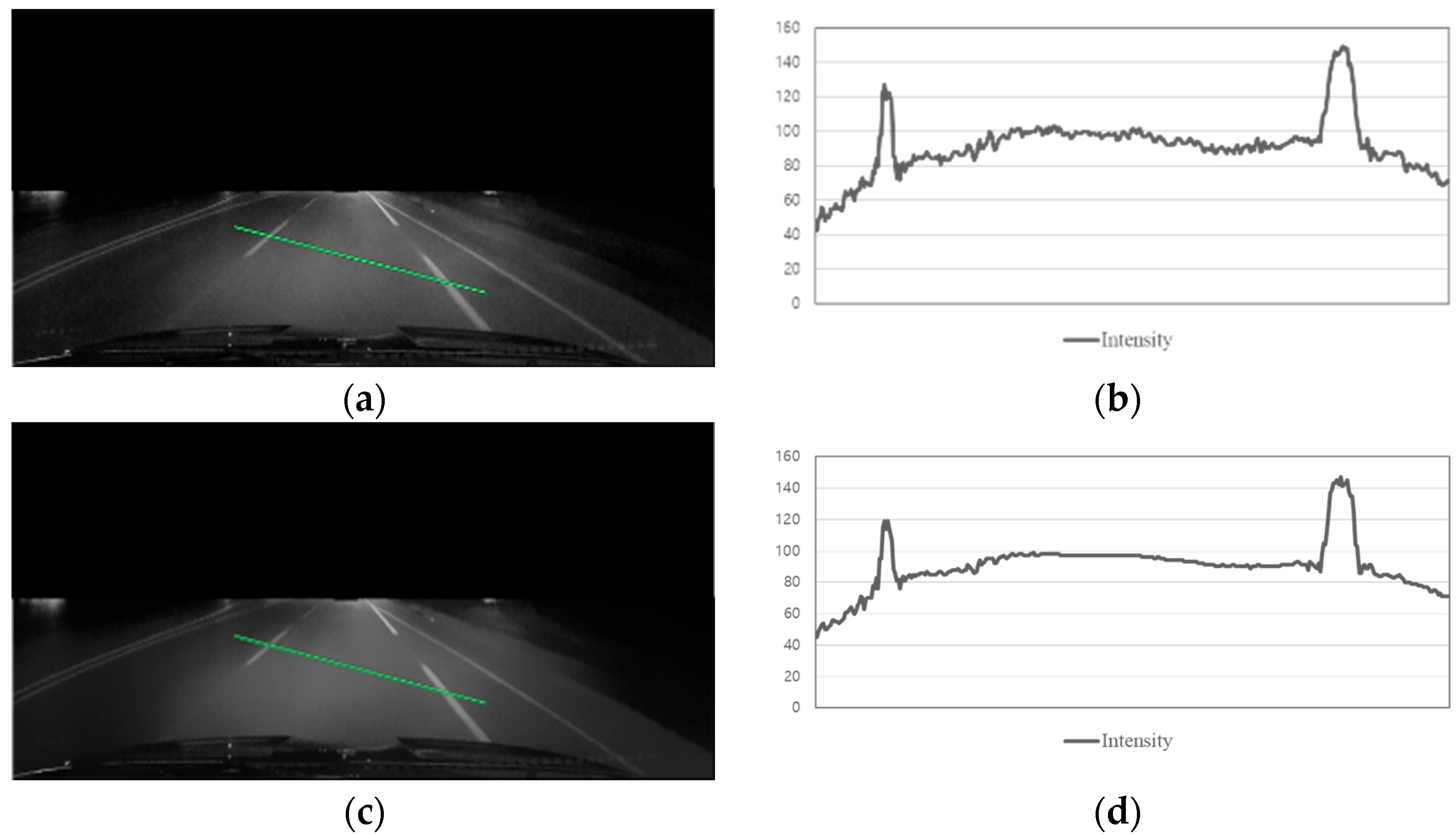
3.2. Lane-Candidate Grouping and Optimal Lane Detection and Tracking

3.2.1. Determination of the Edge and Straight Line

In the preprocessed image with noise suppression and enhanced contrast, the Canny edge detector is employed to detect the edges [7]. As the Gaussian blur step of the Canny edge detection has already been replaced during the noise-reduction process, it is omitted. In the hysteresis thresholding stage, the high thresholding is set to a low value, while the low thresholding is set to a high value, aiming to detect a maximum number of edges while eliminating small ones. These threshold values were determined through experimental analysis. Subsequently, the Hough transform is applied to detect candidate lines from the edge image, as illustrated in Figure 14 [10].

3.2.2. Restriction System and Lane Tracking

As the subsequent step, the final lane is determined through the process depicted in Figure 15, starting from the lane-candidate group obtained using the Hough transform.

The angle and distance restrictions in this paper are determined based on the experimental results shown in Figure 16. The experiment involved analyzing 1000 images. Figure 16 displays the outcome of applying k-means clustering to the point cloud representing the detected lanes. The scattered points represent the angles and distances of the lanes detected by this method without the restriction system. The angle (θ) and distance (D_dist) are calculated using Equations (4) and (5), respectively.

$$\theta ={\Vert \tan }^{-1}\frac{y_{line}}{x_{line}}\Vert ,$$

(4)

$$D_{dist}=\Vert \frac{C_{line}-C_{img}}{W_{img}}\Vert ,$$

(5)

where $y_{lane}$ is the line height, $x_{line}$ is the line width, $C_{line}$ is the coordinate of the line’s center point, $C_{img}$ is the coordinate of the image’s center point, $w_{img}$ is the image’s width length, and $D_{dist}$ indicates the distance of the lane from the center of the image.

The k-means clustering algorithm is used in this study to group the data into k clusters based on minimizing the variance of the distance between each cluster [35]. The light-green cluster in the k-means clustering result is considered as the lane distribution. To improve the lane-detection rate, the angle ($\theta$) and distance (D_dist) are restricted to a range of 0.4 to 0.8 and 0.06 to 0.4, respectively. These constraints increase the probability of detecting the actual lanes among the detected lines. While these restrictions are stringent, it is possible that a lane may not be detected in a single frame. However, the Kalman filter is used to estimate the lane based on the information from previous frames.

In the previous step, two lanes are obtained and updated using the Kalman filter. This lane information is used for the Kalman prediction in the next frame. The lane information also corrects the estimated lane from the previous frame using the currently observed information [11]. In cases where an appropriate lane is not detected in the current frame due to strong external light interference, the Kalman tracking result from the previous frame is used. When the Kalman filter is updated and lane information is not detected in the current frame, the lane of the current frame is estimated using only the previous data without a correction value. However, due to the robustness of the Kalman filter, stable detection and tracking are possible under certain frame conditions as long as the lane does not change abruptly. Overall, this approach prevents the degradation of the Kalman filter’s performance by avoiding false information about the lane during the prediction phase.

4. Simulations

4.1. Experimental Results

The proposed method was implemented on a PC with the following specifications: an Intel i5-6500 processor, 8GB RAM, running Python version 3.9.12 on Windows 10. Additionally, the U-Net ConvLSTM and DSUNet methods for comparisons have been trained and executed in a different computer environment. This environment consisted of an Intel i9-11900K processor, 32 GB RAM, and an RTX 4090 GPU. The U-Net ConvLSTM and DSUNet implementation utilized Python version 3.9.12 on Linux Ubuntu version 22.0.4.s.

Figure 17, Figure 18, Figure 19 and Figure 20 present the comparison results among various lane-detection methods including the U-Net ConvLSTM and DSUNet neural network architectures. The DSUNet is a modification of the U-Net architecture, where all layers except the first layer are replaced with depthwise and pointwise convolution layers from the standard convolution layer structure. Additionally, drop-out is incorporated to prevent overfitting. The conventional method incorporates the Gaussian filter, Canny edge, Hough transform, and Kalman filter [2,10,11]. Furthermore, the U-Net ConvLSTM is a neural network architecture that replaces the skip connection part of the U-Net with long short-term memory (LSTM) [29]. The neural network was trained using a dataset comprising 401,052 images. As mentioned earlier, the experiments were conducted by comparing different environments. These environments can be broadly categorized as follows: cases where the image contains a wiper, cases where the lane markings on the road are not clearly visible due to rainwater, cases where there are obstructions such as guidelines in the road area, and cases where the road area is overexposed by headlights from vehicles and other factors during nighttime.

Figure 17 demonstrates the results of the lane detection when a wiper is present in the image. The U-Net ConvLSTM method struggles to detect the lanes accurately. In the case of the DSUNet method, it increases the number of unnecessary detections, such as pedestrian crossings or windshield wipers. The conventional method achieves relatively successful lane detection. However, in videos where the windshield wiper is constantly moving, the detection results are not satisfactory due to wiper interference. In contrast, the proposed method performs well in both scenarios, accurately detecting the lanes even when rainwater reflection or wiper interference is present. Figure 18 shows the results of lane detection in the case where the road area is heavily reflected due to rainwater. In this case, where the reflection is severe, other methods fail to detect the lane markings, while the proposed method successfully identifies the lane markings.

Figure 19 displays the results of lane detection in the case where there are lines other than lane markings present in the road area, causing interference with the detection process. DSUNet shows a better performance compared to U-Net ConvLSTM as it avoids detecting irrelevant lines and provides more accurate lane detection. Figure 20 demonstrates the challenges posed by dark environments where there is no sunlight and the lane area is overexposed by headlights from vehicles and streetlights. DSUNet demonstrates a certain level of robust detection even under challenging conditions. On the other hand, the U-Net ConvLSTM method, due to severe noise, fails to detect lanes in several areas. Additionally, the conventional method struggles to properly detect the lanes when they are obstructed by guidelines before entering tollgates. In contrast, the proposed method consistently and reliably detects the lanes in all situations, overcoming these challenges effectively.

4.2. Objective Assessment

To evaluate the performance of the proposed method quantitatively, we measured the detection rate. We conducted the evaluation in four different scenarios: cases where the front view was obstructed by the wiper, cases where the road area was reflected by rainwater, cases where there were other lines present in the road area, and cases where the road area was overexposed by multiple light sources. In each scenario, we evaluated the detection of both left and right lanes, resulting in a total of 400 images (100 images for each scenario). The evaluation method involved comparing the detected lanes with the actual lanes. If the detected lanes closely matched the actual lanes, they were considered true; otherwise, they were considered false. The evaluation criteria are the same as in Figure 21. We separately evaluated the left and right lanes and then combined them to assess if they correctly represented the direction of the actual vehicle. The evaluation results are presented in

Table 1. Comparison of lane-detection rate.

	Left Lane (Conv/DSUNet/LSTM/Prop)	Right Lane (Conv/DSUNet/LSTM/Prop)
Wiper	0.49/0.72/0.57/0.65	0.40/0.63/0.54/0.69
Rainy surface	0.33/0.51/0.50/0.54	0.26/0.70/0.74/0.73
Overexposed	0.64/0.82/0.55/0.94	0.61/0.88/0.50/0.93
Guideline	0.35/0.86/0.59/0.84	0.03/0.75/0.65/0.70

. In the results, compared to the U-Net-based method, about 34% in the left-lane case and about 30% in the right-lane case were observed. In the case of DSUNet, there is little difference compared to the proposed method in the score, and in some cases, even better results can be observed. However, the proposed method is more suitable for the goal of detecting only the lanes present in the driving road area.

5. Conclusions

This paper aimed to identify daytime and nighttime periods in video footage and set optimal parameters for lane detection under challenging conditions. The proposed approach involved utilizing the restriction system to determine the most probable lane lines from the detected candidates in the edge image. The position information was then updated using the Kalman filter to predict the lane position in the next frame.

In the experiments, it was observed that the proposed approach exhibited slightly more stability compared to conventional methods, U-Net ConvLSTM, and DSUNet. This confirms the effectiveness of distinguishing between daytime and nighttime periods, setting appropriate parameters, maximizing contrast using MSR, and selecting lanes with the proposed restriction system, achieving successful and stable lane detection in challenging conditions.

However, the proposed approach in this paper has limitations in detecting curved lanes, as the Hough transform used can only identify straight lines in the edge image. To address this limitation, this paper suggests exploring pixel-level segmentation techniques for accurate detection of curved lanes. This can involve subdividing the lane-detection area into smaller segments and representing curves using multiple lines or adopting alternative approaches.

As demonstrated in this paper, deep learning is not always superior in all scenarios. The experiments revealed that while deep learning requires powerful GPUs, extensive datasets (400,000 images), and long training times, the proposed approach achieved comparable or even better results without the need for dedicated GPU devices, large datasets, or extensive training time. This highlights the practicality and effectiveness of the proposed approach in challenging lane-detection scenarios.

References

1. Lee, D.-K.; Lee, I.-S. Performance Improvement of Lane Detector Using Grouping Method. J. Korean Inst. Inf. Technol. 2018, 16, 51–56. [Google Scholar] [CrossRef]
2. Yoo, H.; Yang, U.; Sohn, K. Gradient-enhancing conversion for illumination-robust lane detection. IEEE Trans. Intell. Transp. Syst. 2013, 14, 1083–1094. [Google Scholar] [CrossRef]
3. Stoel, B.C.; Vossepoel, A.M.; Ottes, F.P.; Hofland, P.L.; Kroon, H.M.; Schultze Kool, L.J. Interactive Histogram Equalization. Pattern Recognit. Lett. 1990, 11, 247–254. [Google Scholar] [CrossRef]
4. Hines, G.; Rahman, Z.; Woodell, G. Single-Scale Retinex Using Digital Signal Processors. In Proceedings of the Global Signal Processing Conference, San Jose, CA, USA, 25–29 October 2004; pp. 1–6. [Google Scholar]
5. Petro, A.B.; Sbert, C.; Morel, J.-M. Multiscale Retinex. Image Process. Line 2014, 4, 71–88. [Google Scholar] [CrossRef]
6. Sultana, S.; Ahmed, B. Robust Nighttime Road Lane Line Detection Using Bilateral Filter and SAGC under Challenging Conditions. In Proceedings of the 2021 IEEE 13th International Conference on Computer Research and Development (ICCRD), Beijing, China, 5–7 January 2021; pp. 137–143. [Google Scholar] [CrossRef]
7. Canny, J. A Computational Approach to Edge Detection. IEEE Trans. Pattern Anal. Mach. Intell. 1986, 6, 679–698. [Google Scholar] [CrossRef]
8. Aminuddin, N.S.; Ibrahim, M.M.; Ali, N.M.; Radzi, S.A.; Saad, W.H.M.; Darsono, A.M. A New Approach to Highway Lane Detection by Using Hough Transform Technique. J. Inf. Commun. Technol. 2017, 16, 244–260. [Google Scholar] [CrossRef]
9. Lee, C.-Y.; Kim, Y.-H.; Lee, Y.-H. Optimized Hardware Design Using Sobel and Median Filters for Lane Detection. J. Adv. Inf. Technol. Converg. 2019, 9, 115–125. [Google Scholar] [CrossRef]
10. Illingworth, J.; Kittler, J. A Survey of the Hough Transform. Comput. Vision, Graph. Image Process. 1988, 44, 87–116. [Google Scholar] [CrossRef]
11. Borkar, A.; Hayes, M.; Smith, M.T. Robust Lane Detection and Tracking with Ransac and Kalman Filter. In Proceedings of the 16th IEEE International Conference on Image Processing (ICIP), Cairo, Egypt, 7–10 November 2009; pp. 3261–3264. [Google Scholar] [CrossRef]
12. Guo, J.; Wei, Z.; Miao, D. Lane Detection Method Based on Improved RANSAC Algorithm. In Proceedings of the 2015 IEEE Twelfth International Symposium on Autonomous Decentralized Systems 2015, Taichung, Taiwan, 25–27 March 2015; pp. 285–288. [Google Scholar] [CrossRef]
13. Sander, J.; Ester, M.; Kriegel, H.P.; Xu, X. Density-Based Clustering in Spatial Databases: The Algorithm GDBSCAN and Its Applications. Data Min. Knowl. Discov. 1998, 2, 169–194. [Google Scholar] [CrossRef]
14. Niu, J.; Lu, J.; Xu, M.; Lv, P.; Zhao, X. Robust Lane Detection Using Two-Stage Feature Extraction with Curve Fitting. Pattern Recognit. 2016, 59, 225–233. [Google Scholar] [CrossRef]
15. Lee, S.; Hyeon, D.; Park, G.; Baek, I.J.; Kim, S.W.; Seo, S.W. Directional-DBSCAN: Parking-Slot Detection Using a Clustering Method in around-View Monitoring System. In Proceedings of the 2016 IEEE Intelligent Vehicles Symposium (IV), Gothenburg, Sweden, 19–22 June 2016; pp. 349–354. [Google Scholar] [CrossRef]
16. Ding, Y.; Xu, Z.; Zhang, Y.; Sun, K. Fast Lane Detection Based on Bird’s Eye View and Improved Random Sample Consensus Algorithm. Multimed. Tools Appl. 2017, 76, 22979–22998. [Google Scholar] [CrossRef]
17. Luo, L.B.; Koh, I.S.; Park, S.Y.; Ahn, R.S.; Chong, J.W. A Software-Hardware Cooperative Implementation of Bird’s-Eye View System for Camera-on-Vehicle. In Proceedings of the 2009 IEEE International Conference on Network Infrastructure and Digital Content 2009, Beijing, China, 6–8 November 2009; pp. 963–967. [Google Scholar] [CrossRef]
18. Meng, Z.; Xia, X.; Xu, R.; Liu, W.; Ma, J. HYDRO-3D: Hybrid Object Detection and Tracking for Cooperative Perception Using 3D LiDAR. IEEE Trans. Intell. Veh. 2023, 20, 1–13. [Google Scholar] [CrossRef]
19. Xia, X.; Meng, Z.; Han, X.; Li, H.; Tsukiji, T.; Xu, R.; Zheng, Z.; Ma, J. An Automated Driving Systems Data Acquisition and Analytics Platform. Transp. Res. Part C Emerg. Technol. 2023, 151, 104120. [Google Scholar] [CrossRef]
20. McCall, J.C.; Trivedi, M.M. An Integrated, Robust Approach to Lane Marking Detection and Lane Tracking. In Proceedings of the IEEE Intelligent Vehicles Symposium, Parma, Italy, 14–17 June 2004; pp. 533–537. [Google Scholar] [CrossRef]
21. Apostoloff, N.; Zelinsky, A. Robust Vision Based Lane Tracking Using Multiple Cues and Particle Filtering. In Proceedings of the IEEE IV2003 Intelligent Vehicles Symposium, Columbus, OH, USA, 9–11 June 2003; pp. 558–563. [Google Scholar] [CrossRef]
22. Loose, H.; Franke, U.; Stiller, C. Kaiman Particle Filter for Lane Recognition on Rural Roads. In Proceedings of the 2009 IEEE Intelligent Vehicles Symposium, Xi’an, China, 3–5 June 2009; pp. 60–65. [Google Scholar] [CrossRef]
23. Xiong, L.; Xia, X.; Lu, Y.; Liu, W.; Gao, L.; Song, S.; Yu, Z. IMU-Based Automated Vehicle Body Sideslip Angle and Attitude Estimation Aided by GNSS Using Parallel Adaptive Kalman Filters. IEEE Trans. Veh. Technol. 2020, 69, 10668–10680. [Google Scholar] [CrossRef]
24. Liu, W.; Xia, X.; Xiong, L.; Lu, Y.; Gao, L.; Yu, Z. Automated Vehicle Sideslip Angle Estimation Considering Signal Measurement Characteristic. IEEE Sens. J. 2021, 21, 21675–21687. [Google Scholar] [CrossRef]
25. Xia, X.; Hashemi, E.; Xiong, L.; Khajepour, A. Autonomous Vehicle Kinematics and Dynamics Synthesis for Sideslip Angle Estimation Based on Consensus Kalman Filter. IEEE Trans. Control Syst. Technol. 2023, 31, 179–192. [Google Scholar] [CrossRef]
26. Firdaus-Nawi, M.; Noraini, O.; Sabri, M.Y.; Siti-Zahrah, A.; Zamri-Saad, M.; Latifah, H. DeepLabv3+_Encoder-Decoder with Atrous Separable Convolution for Semantic Image Segmentation. Pertanika J. Trop. Agric. Sci. 2011, 34, 137–143. [Google Scholar]
27. Badrinarayanan, V.; Kendall, A.; Cipolla, R. Segnet: A Deep Convolutional Encoder-Decoder Architecture for Image Segmentation. IEEE Trans. Pattern Anal. Mach. Intell. 2017, 39, 2481–2495. [Google Scholar] [CrossRef]
28. Neven, D.; De Brabandere, B.; Georgoulis, S.; Proesmans, M.; Van Gool, L. Towards End-to-End Lane Detection: An Instance Segmentation Approach. In Proceedings of the 2018 IEEE Intelligent Vehicles Symposium (IV), Changshu, China, 26–30 June 2018; pp. 286–291. [Google Scholar] [CrossRef]
29. Zou, Q.; Jiang, H.; Dai, Q.; Yue, Y.; Chen, L.; Wang, Q. Robust Lane Detection from Continuous Driving Scenes Using Deep Neural Networks. IEEE Trans. Veh. Technol. 2020, 69, 41–54. [Google Scholar] [CrossRef]
30. Medsker, L.R.; Jain, L.C. Recurrent Neural Networks. Des. Appl. 2001, 5, 64–67. [Google Scholar]
31. Graves, A.; Graves, A. Long Short-Term Memory. Supervised Sequence Labelling with Recurrent Neural Networks; Springer: Cham, Switzerland, 2012; pp. 37–45. [Google Scholar]
32. Lee, D.H.; Liu, J.L. End-to-End Deep Learning of Lane Detection and Path Prediction for Real-Time Autonomous Driving. Signal Image Video Process. 2023, 17, 199–205. [Google Scholar] [CrossRef]
33. Goodfellow, I.J.; Pouget-Abadie, J.; Mirza, M.; Xu, B.; Warde-Farley, D.; Ozair, S.; Courville, A.; Bengio, Y. Generative Adversarial Nets. Adv. Neural Inf. Process. Syst. 2014, 3, 2672–2680. [Google Scholar] [CrossRef]
34. Ghafoorian, M.; Nugteren, C.; Baka, N.; Booij, O.; Hofmann, M. EL-GAN: Embedding Loss Driven Generative Adversarial Networks for Lane Detection. Lect. Notes Comput. Sci. 2019, 11129, 256–272. [Google Scholar] [CrossRef]
35. Hartigan, J.A.; Wong, M.A. Algorithm AS 136: A K-Means Clustering Algorithm. J. R. Stat. Soc. Ser. C Appl. Stat. 1979, 28, 100–108. [Google Scholar] [CrossRef]
Figure 1. Comparison of histogram equalization and histogram stretching.
Applsci 13 09313 g001
Figure 2. The four steps of Canny edge detection. (1) Noise Smoothing through Gaussian Filtering. (2) Compute Gradient Magnitude and Orientation using the Sobel Edge Mask (Sky blue: 337.5~22.5 and 157.5~202.5 degrees, Red: 22.5~67.5 and 202.5~247.5 degrees, Blue: 67.5~112.5 and 247.5~292.5 degrees, Green: 112.5~157.5 and 292.5~337.5 degrees). (3) Non-maximum suppression. (4) Hysteresis Thresholding step detection enhances weak edges near strong edges to form consistent edges by distinguishing strong and weak edges.
Applsci 13 09313 g002
Figure 4. Flow chart of the proposed method.
Applsci 13 09313 g004
Figure 5. Result of ROI: (a) input image; and (b) upper area used for distinguishing between day and night, lower area used for lane detection.
Applsci 13 09313 g005
Figure 6. Comparison of the resulting images after suppressing noise and increasing contrast: (a) inappropriate parameters during the day; (b) appropriate parameters during the day; (c) inappropriate parameters at night; (d) appropriate parameters at night.
Applsci 13 09313 g006
Figure 7. The average pixel value of the upper area in day and night images (experiment for determining the thresholding point).
Applsci 13 09313 g007
Figure 8. Comparison of the line profiles for noise reduction (The green line indicates the position of the line profile): (a) cropped image; (b) cropped image’s line profile; (c) image with suppressed noise using a bilateral filter; and (d) bilateral image’s line profile.
Applsci 13 09313 g008
Figure 9. A comparison for determining the appropriate parameters of a bilateral filter during daytime (The red lines indicate the position of the lane profile, and the red dots represent the boundary of the lane edge): (a) high bilateral filter parameters and MSR with uniform weight on sigma; (b) image (a)’s lane-line profile; (c) low bilateral filter parameters and MSR with uniform weight on sigma; and (d) image (c)’s lane-line profile.
Applsci 13 09313 g009
Figure 10. A comparison for determining the appropriate parameters of a bilateral filter at nighttime (The red lines indicate the position of the lane profile, and the red dots represent the boundary of the lane edge): (a) high bilateral filter parameters and MSR with uniform weight on sigma; (b) image (a)’s lane-line profile; (c) low bilateral filter parameters and MSR with uniform weight on sigma; and (d) image (c)’s lane-line profile.
Applsci 13 09313 g010
Figure 11. Comparison of the line profiles for contrast enhancement (The green line indicates the position of the line profile): (a) blur image; (b) blur image’s line profile; (c) MSR image; and (d) MSR image’s line profile.
Applsci 13 09313 g011
Figure 12. A comparison for determining the appropriate parameters of an MSR during daytime (The red lines indicate the position of the lane profile, and the red dots represent the boundary of the lane edge): (a) low bilateral filter parameters and MSR with uniform weight on sigma; (b) image (a)’s lane-line profile; (c) low bilateral filter parameters and MSR with higher weight on low sigma; (d) image (c)’s lane-line profile; (e) low bilateral filter parameters and MSR with higher weight on high sigma; and (f) image (e)’s lane-line profile.
Applsci 13 09313 g012aApplsci 13 09313 g012b
Figure 13. A comparison for determining the appropriate parameters of an MSR at nighttime (The red lines indicate the position of the lane profile, and the red dots represent the boundary of the lane edge): (a) High bilateral filter parameters and MSR with uniform weight on sigma; (b) image (a)’s lane-line profile; (c) high bilateral filter parameters and MSR with higher weight on low sigma; (d) image (c)’s lane-line profile; (e) high bilateral filter parameters and MSR with higher weight on high sigma; and (f) image (e)’s lane-line profile.
Applsci 13 09313 g013aApplsci 13 09313 g013b
Figure 14. The image created by applying the Canny edge detection to generate an edge image and detecting lane candidates using the Hough transform: (a) a sample with no interfering factors present in the driving area; and (b) a sample with interfering factors present in the driving area.
Applsci 13 09313 g014
Figure 15. Detailed description of the restriction system at each stage (yellow line: Lane candidates, red line: Selected lane from lane candidates, green line: Lane initially selected from lane candidates but restricted due to being too close to the center, blue line: Lane with corrected position using Kalman Filter from the selected red lane.).
Applsci 13 09313 g015
Figure 16. Experiments for determining the Distance factor and Theta factor (result of k-means clustering of distance–theta points cloud). The red arrows indicate the range of Distance and Theta of the lanes (Blue, red, and yellow: information about lines other than the lanes. Green: lane information).
Applsci 13 09313 g016
Figure 17. Experimental results in the case where the wiper obstructs the image: (a) conventional; (b) DSUNet; (c) U-Net ConvLSTM; and (d) proposed method.
Applsci 13 09313 g017
Figure 18. Experimental results in the case where the road is heavily reflected due to rainwater: (a) conventional; (b) DSUNet; (c) U-Net ConvLSTM; and (d) proposed method.
Applsci 13 09313 g018
Figure 19. Experimental results in the case where there are obstructions such as lines other than lane markings in the road area: (a) conventional; (b) DSUNet; (c) U-Net ConvLSTM; and (d) proposed method.
Applsci 13 09313 g019
Figure 20. Experimental results in the case where the road arear is overexposed by headlights from vehicles and other factors during nighttime: (a) conventional; (b) DSUNet; (c) U-Net ConvLSTM; and (d) proposed method.
Applsci 13 09313 g020
Figure 21. Examples of evaluation criteria for lane detection (Yellow: conventional, Purple: DSUNet, Red: U-Net ConvLSTM, Green: proposed method). (a) An example of correctly detecting the left lane; (b) an example of failing to detect both lanes; (c) an example of correctly detecting the right lane; and (d) an example of correctly detecting both lanes.
Applsci 13 09313 g021