Article

Improved Genetic Algorithm for Solving Green Path Models of Concrete Trucks

1
School of Mechanical Engineering, North China University of Water Resources and Electric Power, Zhengzhou 450045, China
2
School of Management and Economics, North China University of Water Resources and Electric Power, Zhengzhou 450045, China
*
Authors to whom correspondence should be addressed.
Appl. Sci. 2023, 13(16), 9256; https://doi.org/10.3390/app13169256
Submission received: 24 July 2023 / Revised: 8 August 2023 / Accepted: 10 August 2023 / Published: 15 August 2023

Abstract

:
In this paper, for the problem of high total fuel consumption of distribution trucks when multiple concrete-mixing plants distribute concrete together, we established a green fuel consumption model for distribution trucks and solved the model with an improved genetic algorithm to obtain a green distribution scheme for trucks. Firstly, the fuel consumption model is established for the characteristics of commercial concrete tankers; secondly, the adaptive elite retention strategy, adaptive crossover, mutation operator, and immune operation are added to the genetic algorithm to improve it; and finally, the model is solved to obtain the green distribution scheme. The total fuel consumption in this experiment was 189.6 L when the green distribution scheme was used; compared to the total fuel consumption under the original scheme (240 L), the total fuel consumption was reduced by 21.25%. The experimental results show that the total fuel consumption of delivery trucks can be significantly reduced based on the established green fuel consumption model, and the improved genetic algorithm can effectively solve the model.

1. Introduction

In recent years, it has become a common vision of mankind to reduce greenhouse gas emissions to achieve carbon neutrality and protect the environment. In 2019, the energy consumption of China’s transportation sector accounted for 17.2%, and vehicle fuel emission is one of the main causes of air pollution [1]. Commercial concrete companies usually use concrete trucks to deliver concrete to construction sites. With the increase in demand for concrete, it has become a trend for multiple mixing plants to serve customers together. Therefore, it is of significant importance to develop a green path model for concrete vehicles and study green distribution solutions for concrete vehicles to reduce fuel consumption/carbon emissions. The vehicle-routing problem (VRP) was first proposed in [2]. In order to adapt to the development of low-carbon logistics, the concept of the green vehicle-routing problem (GVRP) was proposed in [3]. Liu et al. divided GVRP problems into the green-VRP, pollution routing problem, and VRP in reverse logistics [4]. In order to solve the GVRP, scholars have conducted a lot of research on building green models and algorithms for solving them [5,6,7]. Peng et al. proposed the memetic algorithm (MA) based on machine learning to enhance the local search capability and a greedy algorithm to generate high-quality offspring [8]. Some scholars study the factors that affect vehicle fuel consumption, and establish a reasonable mathematical model of vehicle dispatching to guide the realistic dispatching of vehicles, to reduce vehicle fuel consumption. Since there are many factors affecting vehicle fuel consumption/carbon emissions during realistic dispatching, such as vehicle speed, load, distance, road gradient, ambient temperature, and traffic conditions [9], scholars have conducted numerous studies. Hu et al., combining this with the actual congestion condition of urban roads, and taking into account the road speed, vehicle load, and vehicle driving distance, established the GMDVRP model, aiming at the minimum total fuel consumption cost, and proposed a learning ant colony optimization algorithm (ACO) to solve the problem [10]. Under the background of emergency rescue, Zhang et al. established a multi-objective MDVRP model with capacity constraints, taking the minimum carbon emissions, travel time, and total cost of vehicles as the optimization objectives, and solved it with a genetic algorithm (GA) [11]. Li et al. built a multi-objective MDVRP model with capacity and vehicle constraints by comprehensively considering the carbon emission cost, vehicle travel time, and maximum income, and solved it with an improved ACO [12]. Yao et al. studied the influence of vehicle speed on carbon emissions in the context of sustainable development [13]. Facing various types of GVRP problems, Zhou et al. classified the models of the GVRP into the fuel-consumption/carbon-emission-minimization VRP, integrated-cost-minimization VRP, and multi-objective VRP based on the objective function of the GVRP model [14]. Raafat et al. classified the VRP and its variants solved using the meta-heuristic algorithm, and sorted out and analyzed the application of the meta-heuristic algorithm in solving different vehicle-routing problems [15]. Ana-Maria et al. used four algorithms (GA, ACO, GA-ACO, and ACO-GA) to solve the RVRP under different constraints, and summarized the algorithm with the best optimization effect under different constraints through analysis [16]. Wang et al. established a VRP model with a flexible path with the goal of minimizing the delivery time by considering the flexibility of the vehicle distribution path, and solved it with an MCTS-GA [17]. Wei et al. built an optimal-path-planning model based on multi-objective factors after summarizing the vehicle optimal path problem, and analyzed the model with a*, a hierarchical algorithm, an ACO, and a GA [18].
The distribution of ready-mixed concrete (RMC) is essentially a vehicle-routing problem. Feng et al. analyzed the factors affecting RMC distribution and built a model based on the GA to solve the optimal distribution scheme with the objective of minimizing the total waiting time of RMC distribution vehicles at the construction site, and, later, they tried to build an RMC-scheduling model by the FMGA and simulation techniques to find the scheduling scheme with the minimum total pouring waiting time of RMC distribution vehicles [19,20], respectively. Yang et al. established a vehicle-scheduling model with the goal of minimizing the interrupted pouring and waiting pouring time at each mixing station, and solved the model with a GA [21]. Kuo [22], aiming at minimizing the total fuel consumption of vehicles, the authors developed a time-dependent VRP (TDVRP), considering the vehicle speed, delivery distances, and load factors, and, also, used a simulated annealing (SA) algorithm to solve the problem. A general concrete delivery model was proposed in [23], but it ignored the time window and vehicle failure factors. Considering vehicles can break down during the distribution of concrete, Yan et al. proposed a model for concrete companies to adjust their plans in time to reduce production costs [24]. However, the difficulty of solving the problem obviously increases when considering the vehicle distribution failure problem. Maghrebi et al. divided the RMC distribution solution process into two parts to reduce the complexity of the problem [25]. Although, for [26], from the perspective of multiple mixing plants supplying multiple sites and considering the work of mixers, a mathematical model with the objective of minimum fuel during RMC distribution is established and solved by a bee algorithm (BA), the article defaults to a consistent volume for all concrete trucks. The summary of the vehicle-routing problem is shown in Table 1.
While scholars have made significant research achievements, there is still a lack of studies on how different concrete mixer trucks can collaborate to supply concrete and reduce total fuel consumption during vehicle distribution. In this paper, based on a comprehensive consideration of the impact of vehicle type, vehicle load, vehicle travel speed, and vehicle travel distance on vehicle fuel consumption, a green path model for the concrete truck mixer with the goal of minimizing total fuel is established and solved with an improved genetic algorithm. The main research objective of this paper is to reduce fuel consumption during the concrete distribution process in order to realize low-carbon concrete distribution. The main contributions of this paper are as follows:
  • The vehicle fuel consumption of a concrete tanker was modeled;
  • A low-carbon collaborative distribution model of multi-mixing stations was established for the current situation of concrete multi-mixing station distribution;
  • Adaptive elite retention strategies, adaptive crossover, mutation operators, and immune selection have been added to the standard genetic algorithm to improve it;
  • The established low-carbon co-operative distribution model for multiple mixing stations was solved using improved genetic algorithms in combination with concrete enterprise orders.

2. Fuel Consumption Models

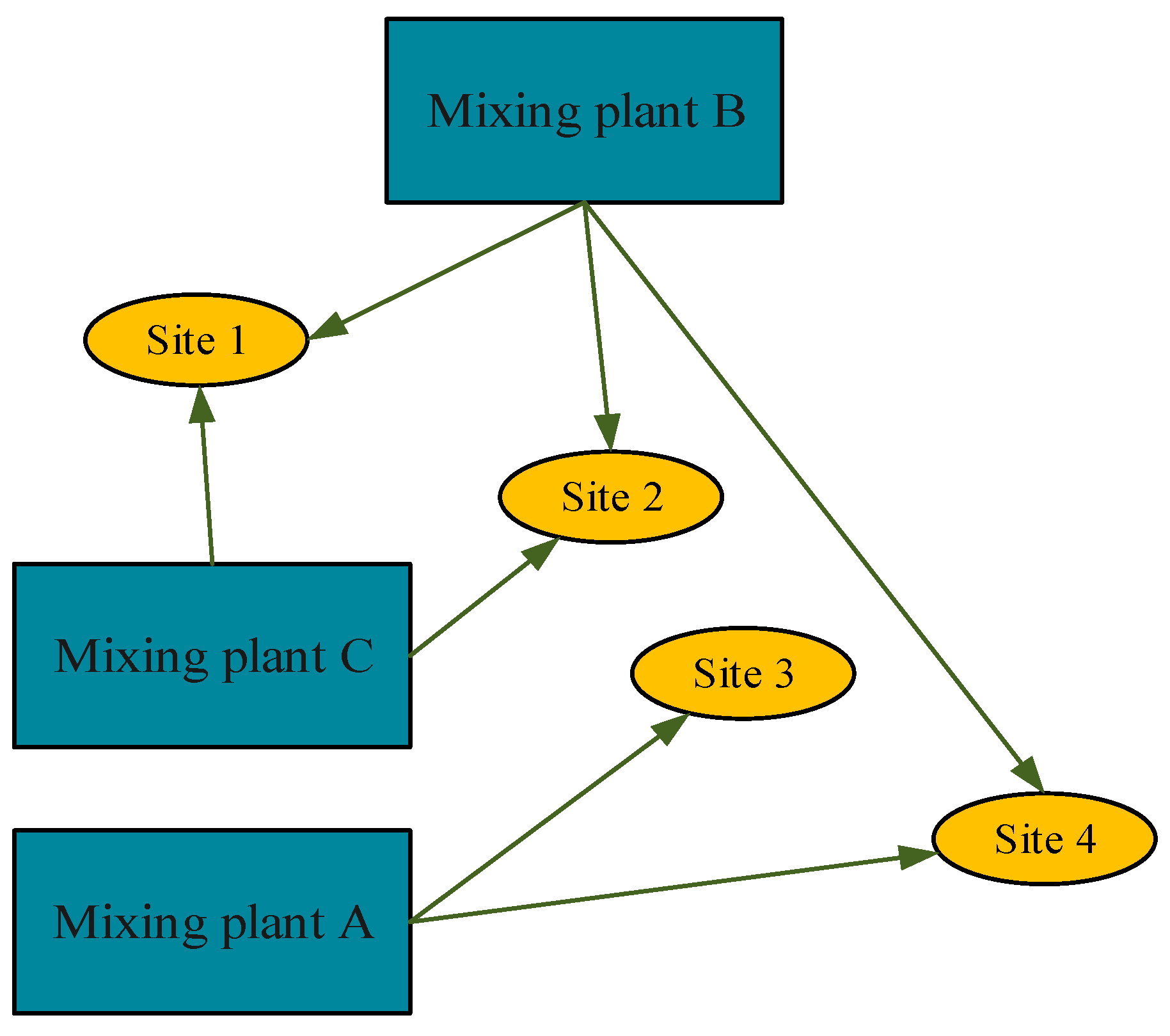
According to the vehicle engine energy consumption model proposed in [27], factors related to the vehicle path will affect the vehicle fuel consumption, such as the vehicle distance traveled, the total weight of the vehicle, and the angle between the vehicle and the road ramp, so the fuel consumption of the concrete truck varies under different distribution schemes. Figure 1 illustrates the co-operative distribution of concrete to four sites by three concrete-mixing plants. The goal of this study is to establish a green distribution path model for dispatching vehicles when multiple concrete-mixing plants deliver concrete to numerous construction sites, by optimizing the vehicle distribution scheme, to reduce the total fuel consumption of the vehicles.
Since vehicle carbon emissions and fuel consumption are positively correlated, the lower the total oil consumption of vehicles during the entire distribution process, the lower the total carbon emissions [28]; hence, the problem solved in this paper belongs to the green VRP. In order to better study the problem, the following assumptions must be established:
(1)
Each concrete distribution truck is allowed to depart from the mixing plant to the customer’s site only once and is not allowed to return;
(2)
The mixing plants are able to produce different grades of concrete in time to meet the needs of each site;
(3)
The maximum transport time required by the site for each mixing plant is the true transport time of the truck;
(4)
Concrete trucks in transit will not interrupt distribution.

2.1. Vehicle Driving Fuel Consumption

Vehicle fuel consumption models include the CMEM, LFCM, and theoretical energy consumption model [27,29,30], respectively. The theoretical energy consumption U x y z is formulated as Equation (1); because of its high confidence and ex situ applicability, this paper derives the corresponding vehicle fuel consumption model based on the theoretical energy consumption model. Considering fuel efficiency, fuel calorific value, and fuel density, there is a conversion relationship between vehicle fuel consumption model and theoretical energy consumption model, as shown in Equation (2). F 1 is fuel consumption per unit distance (L/km), γ f is fuel efficiency, C f is calorific value of fuel (MJ/kg), and ρ f is fuel density (kg/L).
U xyz = η motor e v γ fuel L [ d g Mgsin θ + C i M fr β ad i + C r Mgcos θ ϕ t d r λ s + 0.5 ρ A f C d V r 2 β d a + ( m 2 v 4 R 2 C av ) β λ s d c
F 1 = U xyz / γ f C f ρ f
The following vehicle running state has a small impact on vehicle fuel consumption, so the simplified fuel consumption model is shown in Equation (3):
(1)
Climbing and turning of vehicles on urban roads;
(2)
Acceleration and deceleration of vehicles.
F x = ( 0 . 5 ρ A f C d d a v r 2 β e v η motor + C r ϕ t λ s d r Mge v η motor ) / LC f ρ f
by using the relationship between the average vehicle speed v (m/s), vehicle transportation time T (h), and vehicle travel distance L (km), which is v = L / T , F x , as follows:
F x = ( MC r ϕ t λ s ge v η motor + ( 5 L / 18 T ) 2 × 0 . 5 ρ A f C d β e v η motor ) / C f ρ f
F x : fuel consumption per unit distance, where M s is vehicle mass, M c is loading mass, and M = M s + M c . The symbols associated with Equation (3) are described in Table 2.

2.2. Fuel Consumption of Stirring Tank

The engine power of the concrete mixer truck is divided into two parts: one part is used to drive the vehicle, while the other part drives the stirring tank to rotate. Specifically, the mechanical energy is initially transformed into hydraulic energy by the hydraulic pump, and this hydraulic energy is then transmitted to the hydraulic motor, which converts it back into mechanical energy; the resulting mechanical energy is utilized to drive the stirring tank’s rotation, after the torque is amplified by the reducer. From the above analysis, it can be seen that the stirring tank will also affect vehicle fuel consumption in the process of vehicle distribution. Ignoring the loss during energy conversion, the energy consumption of the stirring tank can be approximately replaced by the output work of the hydraulic motor. To derive the fuel consumption model for the stirring tank, the fuel efficiency and fuel calorific value are combined, as shown in Equation (5). ( W k (MJ): energy consumed by vehicle k stirring tank, and F k : fuel consumption of vehicle k stirring tank.) Table 1 describes the key parameters in the fuel consumption model.
F k = W k / γ f C f ρ f  

2.3. GVRP Model

2.3.1. Objective Function

In order to better describe the objective function, the concrete-mixing plant, concrete demand site, distribution vehicles, and other related symbols are explained as follows:
H i : Concrete-mixing plant i , 1 i n ,
N j : Concrete demand site j , 1 j m ,
Q j : Concrete order quantity of site j (m³),
V k : Concrete truck k , 1 k r ,
V k i j : Concrete truck k from mixing plant i to site j ,
M k i j : The total weight of the V k i j (t),
M z k i j : Rated load of the V k i j (t),
M s k : Self-weight of the V k i j (t),
L i j : The distance traveled by V k i j   (km),
T i j : The time required from mixing plant i to site j (h),
P k : Rated power of V k hydraulic motor,
k i : Vehicle number k belongs to the vehicle set of mixing plant i ,
k i : Vehicle number k doesn’t belongs to the vehicle set of mixing plant i ,
X i k : Decision variable.
X i k = { 1   k i 0   k i
The objective function is established by combining the fuel consumption models for truck driving and stirring the tank, mentioned previously.
When multiple mixing plants co-operate to transport concrete to multiple sites, the total fuel consumption of all trucks driving is as follows:
      F x = i = 1 n j = 1 m k = 1 r L ij · X ik · F x
Integrate the known factors affecting the fuel consumption of the truck driving as f 1 , and f 2 ; the final truck driving fuel consumption as follows:
f 1 = ( C r ϕ t λ s ge v η motor ) / C f ρ f
f 2 = 0 . 5 ρ A f C d β e v η motor / C f ρ f
F x = i = 1 n j = 1 m k = 1 r L ij X ik [ M kij f 1 + ( 5 L ij / 18 T ij ) 2 f 2 ]
When multiple mixing plants co-operate to transport concrete to multiple sites, the total fuel consumption of all trucks stirring the tank is shown in Equation (8).
F k = i = 1 n j = 1 m k = 1 r X ik ( P k T ij / C f ρ f γ f )  
The objective function consists of two parts, which are calculated as follows:
Z =   F x +   F k

2.3.2. Constraints

The following constraints must be established in order for the green path model for concrete trucks to explore how to reduce the overall fuel consumption of distribution trucks while still meeting the demand for concrete at each site. The symbol descriptions and values in the model are shown in Table 3.
(1)
The total output of the concrete-mixing plant should meet the total demand of the total customer sites:
k = 1 r i = 1 n j = 1 m M ckij j = 1 m Q j
(2)
The quantity of delivery from the mixing plant to the customer’s site exceeds the customer’s demand:
k = 1 r i = 1 n M zkij Q j
(3)
Weight constraint:
M kij = M sk + M zkij
(4)
Total number of trucks constraint:
i = 1 n V kij r

3. Model Solving

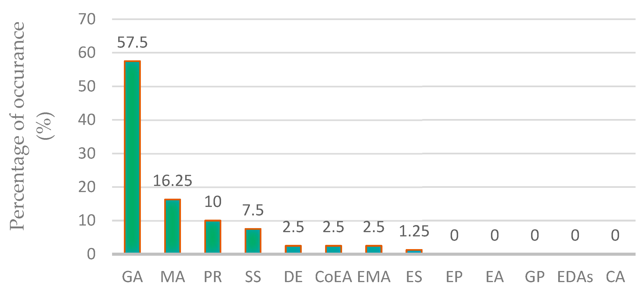
The vehicle-routing problem is an NP-hard problem but metaheuristic algorithms can efficiently find the approximate optimal solution for the VRP in actual execution time. R. E. et al. classified and summarized VRP articles published from 2009 to 2017 in [15]. They found that, in articles using population-based metaheuristic algorithms to solve VRP, evolutionary computation (EC) accounted for 57.1%, while swarm intelligence (SI) accounted for 42.9%. They calculated the usage of each algorithm under the EC strategy, as shown in Figure 2.
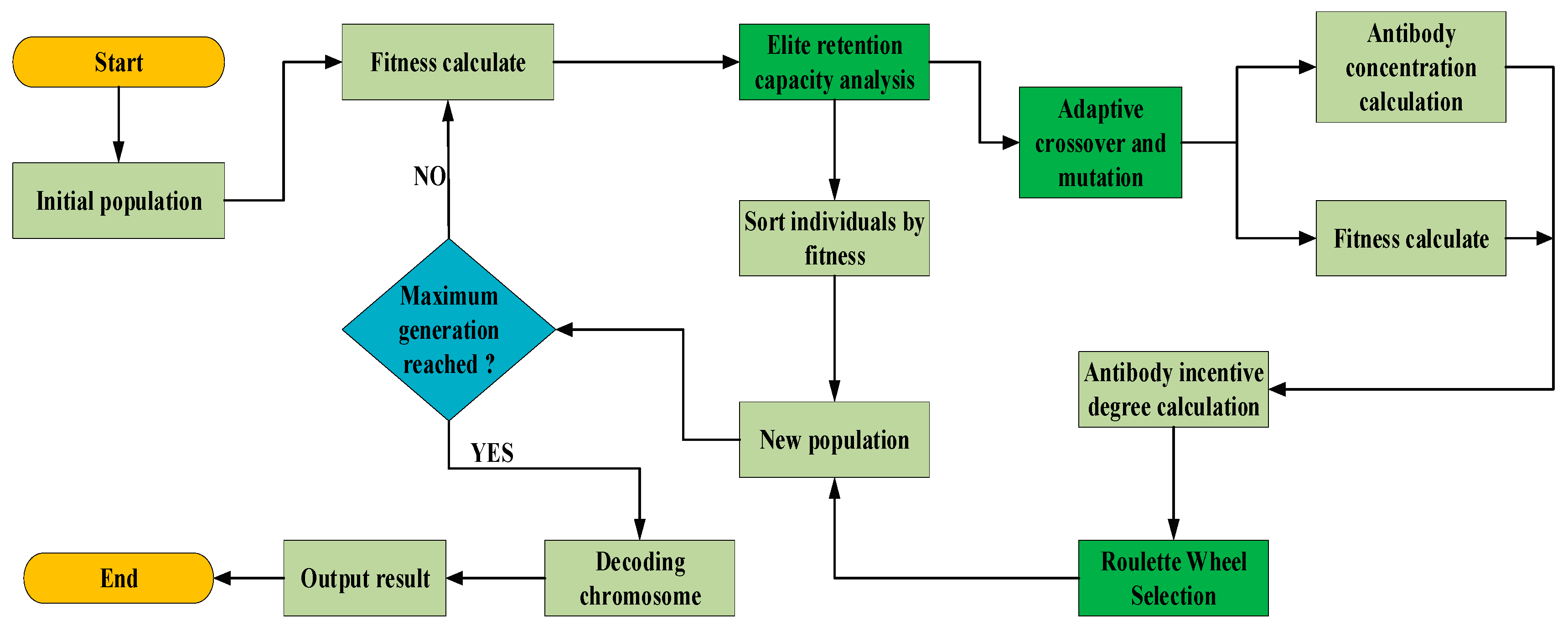
From Figure 2, we can see that the GA is most commonly used for solving the VRP based on population evolution. Since the GA has problems such as slow convergence and, when the crossover and mutation probabilities are stable, it is easy to fall into the local optimal solution [31], this study improved the genetic algorithm to solve the GVRP model provided in this paper. A small mutation probability in the GA is detrimental to population diversity, but a high mutation probability can make the algorithm difficult to converge; a higher crossover probability is advantageous to population diversity but raises the risk of eliminating good individuals [32]. In order to solve the above model better, this study makes four improvements to the GA:
(1)
A new method of preserving superior individuals based on the variable capacity of population size and fitness was introduced in combination with the elite reservation strategy proposed in [33].
(2)
In combination with the adaptive crossover and mutation operators proposed in [34], a new method was introduced to automatically adjust the Pc (crossover probability) and the Pm (mutation probability) based on the individual fitness and the average fitness of the population.
(3)
The immune operator was introduced after crossover and mutation operations to improve the global search ability of the GA. Immune selection selects antibodies according to the antibody incentive degree with a roulette wheel method.
(4)
An adaptive elite retention strategy before crossover and mutation manipulation was introduced.
Individuals are chosen using the roulette wheel selection in this research and are coded in two layers of real numbers. The structure of the improved genetic algorithm is as shown in Figure 3.

3.1. Fitness Value

The research objective of this study is the minimum fuel consumption of the truck in the distribution process. If the fitness value takes the inverse of the objective function, the total fuel consumption decreases as the individual fitness value increases. Individual fitness values are calculated based on whether they satisfy the constraints; if an individual does not satisfy constraints, it is necessary to penalize it by reducing its fitness value as in Equation (10). Individuals that breach the constraints will be eliminated during the evolutionary process because the smaller the total fuel consumption is, the greater the individual fitness value is, and the more likely it is to be retained in the next generation.
f j = { 1 / Z j   if   yes ( 1 / Z j ) 2   if   not
f j : fitness value of individual j ; and Z j : total fuel consumption of individual j .

3.2. Code and Adaptive Strategy

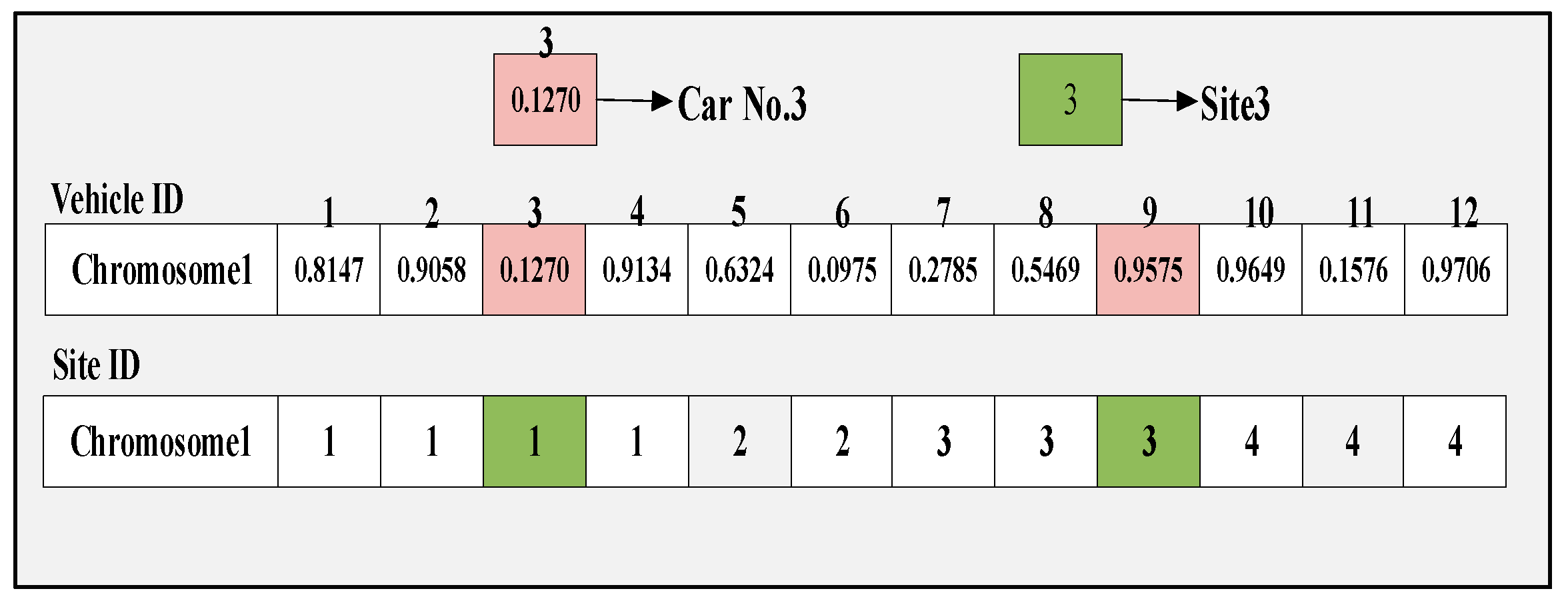
A two-layer real number coding strategy is adopted in this paper, with the first layer representing transport trucks and the second layer representing construction sites. The first layer of codes is related to mixing plants, and the second layer of codes is related to the number of trucks received at each site. The two layers of codes are equal in length and are determined by the total number of trucks received at each site. Since different random numbers in the first layer of encoding represent trucks belonging to different mixing plants, after decoding, the corresponding mixing plants deliver trucks to the target site in the order of random numbers from smallest to largest. For example, as seen in Figure 4, there are 12 trucks, and the number of trucks received at each of the four sites is 4, 2, 3, and 3, respectively. 3→1 and 9→3 denote that concrete is distributed to Sites 1 and 3, respectively, by Truck 3 of the mixing plant and Truck 9 of the other mixing plant.

3.2.1. Elite Retention

The elite retention capacity is determined by the population size and average fitness of the population. The number of elite retention individuals is shown in Equation (11). According to the equation, when the population’s overall fitness value is low, more elite people will be retained to speed algorithm convergence; when the population’s overall fitness value is high, fewer elite people will be retained to increase population diversity.
The adaptive elite retention strategy is shown in Algorithm 1. ( f max : maximum fitness value, f min : minimum fitness value, f a : average fitness value, α : integers greater than 1, and M: population size).
  N e = ceil [ M · ( f max f a ) / α · ( f a f min ) ]
Algorithm 1: Adaptive elite retention strategy
Input: Population fitness: fit; population size: M; population: pop;
Output: N_pop
1: Fit = sort (fit, ‘descend’)
2: Fmax = Fit (1), Fmin = Fit(end), fa = sum (Fit)/M
3:   Ne = ceil [ M ( fmax fa ) / α · (fa−fmin)]
4: In = zeros (Ne,1)
5: F = Fit (1: Ne)
6: for i = 1: Ne
7:   In(i) = find(fit == F(i))
8:   N_pop (i, :)=pop(index(i), :)
9: end

3.2.2. Adaptive Crossover and Mutation Operators

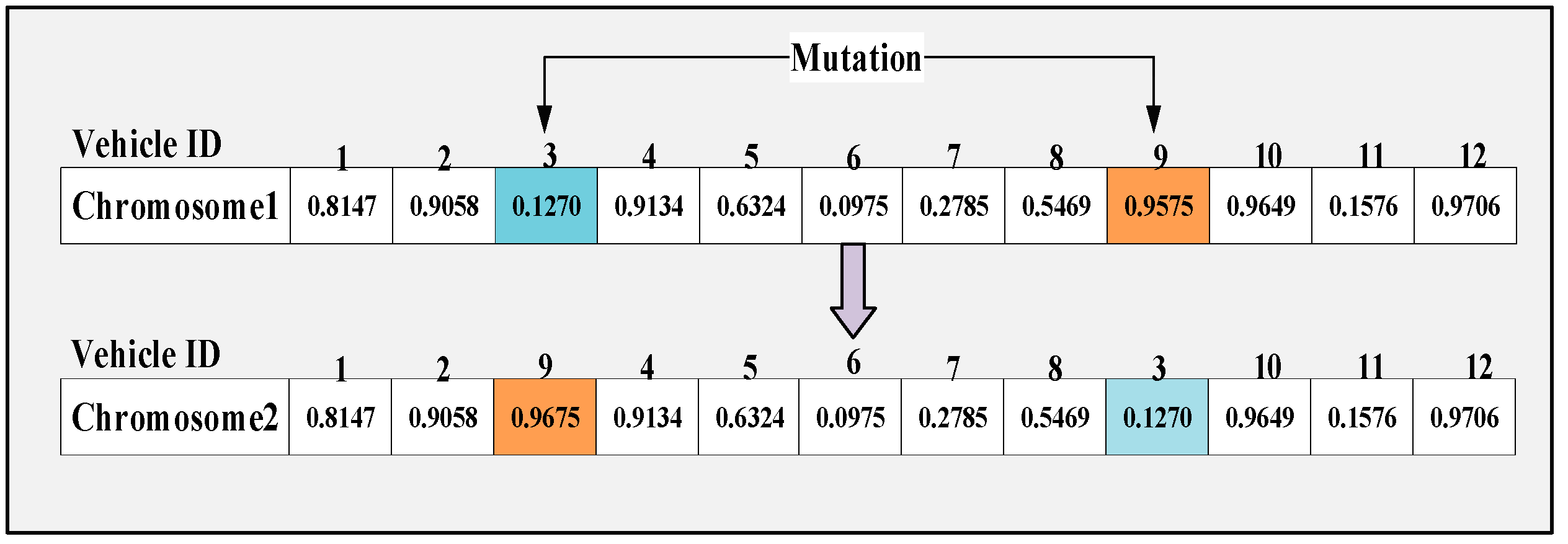
The adaptive crossover operator and adaptive mutation operator are determined by the average fitness of the population, the maximum fitness of the population, etc., as shown in Equations (12) and (13), respectively, so crossover and mutation operators can make adaptive adjustments according to the evolution degree of the population. Inverted mutation and single-point crossover are methods utilized in this paper. The crossover operation of the second layer of encoding is shown in Figure 5, and the mutation operation of the first layer is shown in Figure 6. Crossover probability: p c 1 < p c 2 , and mutation probability: p m 1 <   p m 2 .
P c = { P c 1 + ( P c 2 P c 1 ) sin ( f max f i f max f a π 2 ) ;   f i f a P c 2 ;   f i   <   f a
P m = { P m 1 + ( P m 2 P m 1 ) sin ( f max f i f max f a π 2 ) ;   f i f a P m 2 ;   f i   <   f a
The following information can be derived from the expressions for p c and p m :
(1)
Individuals are more likely to enter the next generation when their fitness value is higher than the average, and, conversely, they are more likely to be displaced.
(2)
In the early stage of the algorithm, since the individuals are randomly generated and the fitness values are less, the use of a larger crossover and mutation probability facilitates the generation of better individuals.
(3)
In the late stages of the algorithm, individuals who have high fitness values, and adopt a smaller crossover and mutation probability are useful for reserving the good individuals and also contributing to enhancing the algorithm’s search efficiency.

3.3. Immune Operator

The affinity between antibodies in immune selection reflects the similarity between antibodies, which is used to determine whether antibodies should be promoted or suppressed. As shown in Equation (14) the affinity function Aff ij is designed for the above antibodies. The first layer of antibody coding is arranged in a fixed way, and only the alleles in the second layer of coding need to be compared to determine Aff ij .
Aff ij = 1 L · t = 1 L t
  t = { 1 ,   ab i , t = ab j , t 0 ,   ab i , t ab i , t
a b i , t and a b j , t represent gene t of antibody i and antibody j , respectively. ( L : coding length of antibody.) Obviously, the range of Aff ij is [0,1], and the larger the value is, the more similar the two antibodies are. Aff ij is the basis for deducing Den i (concentration of antibodies). Den i can indirectly reflect the degree of population diversity, as shown in the following Equations (17) and (18). ( λ : a preset threshold).
Den i = 1 M j = 1 M S ij
S ij = { 1 ,   Aff ij     λ 0 ,   Aff ij   <   λ
The purpose of the immune operator is to select antibodies with a higher degree of incentive to increase the diversity of the population. According to the calculation (Equation (18)) of the incentive degree, when an antibody’s affinity is high but its concentration is low, the value of p m i is relatively large, and the antibody is more easily selected when using roulette wheel selection; on the contrary, antibodies are not easily selected.
  p mi = f i / ( Den i + 1 )
The performance of the improved algorithm proposed in this paper is related to the size of the four preset parameters mentioned above, so the values of the preset parameters are very critical in practical use. In this paper, the improved genetic algorithm adopts double-layer real number coding and uses single-point crossover and mutation to enrich the population diversity. In the actual use of the improved genetic algorithm, firstly, it is necessary to select the appropriate coding method to initialize the population according to the actual problem, and, secondly, selecting the appropriate crossover and mutation methods according to different problems will improve the performance of the algorithm.
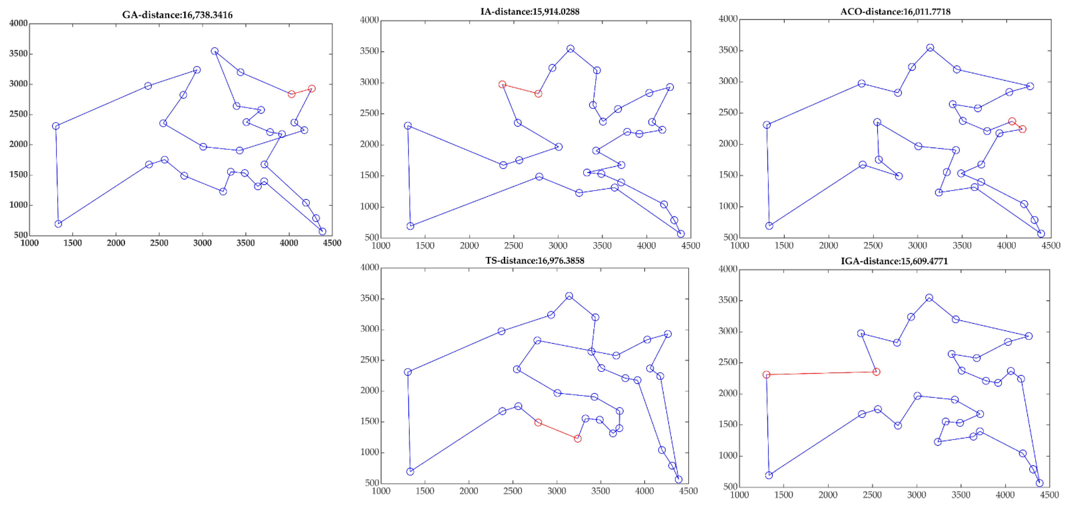
In order to verify the performance of the improved genetic algorithm proposed in this paper, we solved the same function with several metaheuristics (GA, DE, IA, and POS) and compared the results. F ( x ) = min i = 1 10 x i 2   ( 20 x i 20 ) . The values of the relevant algorithm parameters and the optimization results are shown in Table 4, from which it can be seen that the optimal solution solved by the IGA is closer to the exact solution and converges faster. Meanwhile, we solved the same TSP with the GA, ACO, IA, TS, and IGA; the co-ordinates of 31 cities in this problem are shown in Table 5, the final optimized path of each algorithm is shown in Figure 7, and the values of each algorithm parameters and the optimization results are shown in Table 6. By comparing the results of the traveler’s problem solved by each algorithm, we can conclude that the improved genetic algorithm is faster and best optimized. Based on the performance of the improved genetic algorithm in the above problems, we decided to use the improved genetic algorithm to solve the low-carbon distribution model for multiple mixing stations proposed in this paper.

4. Simulation Experiment

In this section, the order of the enterprises is solved using both the standard genetic algorithm and the improved genetic algorithm proposed in this study on the MATLAB platform. The results of the experiments are also analyzed.

4.1. Simulation Process

A commercial concrete company provided the information about mixing plants, construction sites, and trucks. The information included concrete-mixing plants in three distinct regions, construction sites in four different regions, and three various types of trucks. The four sites’ respective concrete requirements are 48 m3 for Site No. 1, 24 m3 for Site No. 2, 36 m3 for Site No. 3, and 36 m3 for Site No. 4, in that order. The number of receiving trucks at the site is four, two, three, and three times, in that order.
The capacities of the different trucks are 16 m3, 12 m3, and 8 m3; in that order, the truck’s hydraulic motor power is 45 kw, 30 kw, and 20 kw, respectively; and its full load weight is 39.5 t, 27 t, and 18.6 t. The truck configuration of mixing plants are shown in Table 7; the information on mixing plants and sites are shown in Table 8.
We combine information from concrete companies with the above mathematical model and solve the model using the standard GA and improved GA. In order to investigate the four key factors affecting the performance of the improved genetic algorithm, we designed experiments using the orthogonal experiment method, and the results were analyzed by range analysis. The levels of the factors in this experiment are shown in Table 9, and the experiment was selected from the L 16 ( 4 4 ) orthogonal experimental table. This experiment uses the convergence algebra of the algorithm and the total fuel consumption as indicators to evaluate the performance of the algorithm, so the experiment is a multi-index orthogonal experiment. The experiment can be transformed into a single-index orthogonal experiment by the comprehensive evaluation method. The composite score method gives each index a corresponding score according to its importance, and the composite score is used as the total index of the experiment.
The values of the crossover and mutation probabilities in the experiment are taken as follows:
{ P c 1 = P c 0 . 15 ,   P c 2 = P c + 0 . 15 P m 1 = P m 0 . 035 ,   P m 2 = P m + 0 . 035
After multiple experiments and improvements on the MATLAB platform, this experiment set the initial population as 80 and the maximum number of iterations as 300; the test results are shown in Table 10. (CA: convergence algebra, FC: fuel consumption, Mv: membership value, and T: index value.)
Mv = T   -   T min / ( T max   -   T min )

4.2. Experimental Analysis

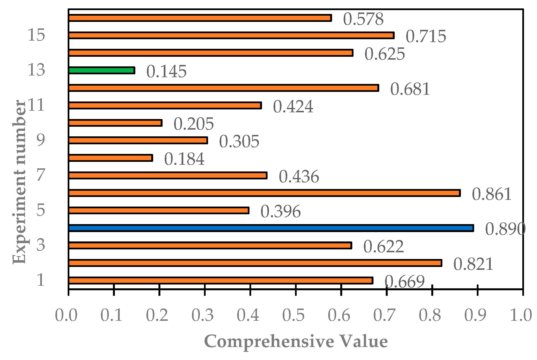
After comprehensive consideration of CV Mv and FV Mv , the range analysis of the test was carried out, as shown in Table 11, and the experiment results were shown in Figure 6. The specific calculation formula of CV is shown below (CV: comprehensive value).
CV = 0.3 CA Mv + 0.7 FC Mv
It can be seen from the Table 11 that K3A < K2A < K4A < K1A, K1B < K3B < K4B < K2B, K4C < K3C < K1C < K2C, K2D < K3D < K1D < K4D; therefore, the optimal levels of α , p c , p m , and λ are 12, 0.55, 0.06, and 0.85. The range values RC < RB < RD < RA; therefore, the value of the mutation probability has the greatest impact on the performance of the improved genetic algorithm. Through the results of range analysis, we can obtain the best horizontal combination: α = 12 , p c = 0.55 , ( p c 1 = 0.4 , p c 2 = 0.7 ), p m = 0.06 , ( p m 1 = 0.025 , p m 2 = 0.095 ), and λ = 0 . 85 .
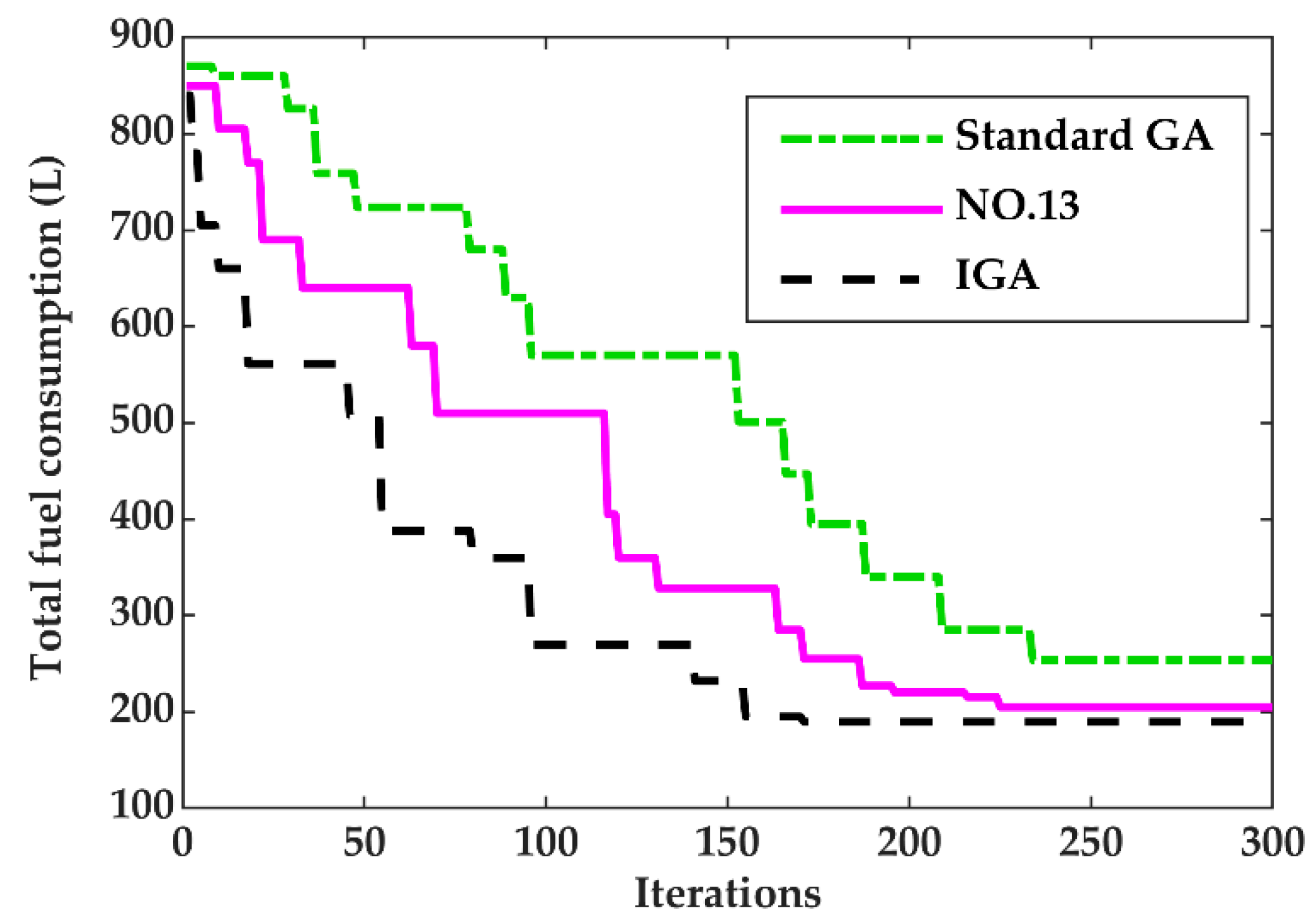
From Figure 8, it can be seen that Experiment No. 13 produced the best results; in order to analyze the performance of the improved genetic algorithm under the optimal level combination, we solved the same enterprise order using the standard genetic algorithm, the improved genetic algorithm in Experiment No. 13, and the improved genetic algorithm under the optimal level combination. When solved by the standard genetic algorithm with Pc = 0.65 and Pm = 0.05, the final experimental results are shown in Figure 9.
From Figure 9, it can be seen that the standard GA converges in approximately 234 generations, while the improved GA converges in 172 generations. Compared with the standard genetic algorithm, the improved genetic algorithm obtains lower total fuel consumption, and the improved genetic algorithm with the best combination of levels obtains the lowest total fuel consumption. The following conclusions can be drawn from the iterative curves of the three algorithms in the figure above:
  • Compared with the standard GA, the IGA has a stronger convergence ability to generate high-quality individuals in the early stage of the algorithm.
  • The IGA converged the solution in 172 iterations and had a 26.45% faster convergence than the standard GA.
  • Compared with the standard genetic algorithm, the final solution obtained by the improved genetic algorithm is better.
  • Compared with Experiment 3, the performance of the improved genetic algorithm under the optimal horizontal combination is improved.
The optimal scheduling scheme is derived after decoding the individual with the maximum fitness value degree as shown in Table 12.
According to the decoded optimal distribution plan, the distribution of the three concrete-mixing plants in this experiment is shown in Figure 10. The specific delivery situation is that concrete-mixing plant A delivers concrete to construction sites 3 and 4, concrete-mixing plant B delivers concrete to construction sites 1, 2, and 3, and concrete-mixing plant C delivers concrete to construction sites 1 and 2.
A comparison of the vehicle distribution routes of the concrete company according to the original plan and the vehicle distribution routes derived from the mathematical model solved by the GA is shown in Table 13.
The objective function value MinZ =   F x +   F k   F k = 189.6   ( L ) under this optimal scheduling scheme indicates that the 12 concrete trucks in this experiment have a total transportation volume of 156 m3; the total fuel consumption is 189.6 L. The enterprise’s original plan’s total fuel consumption is 270 L for the same total demand. Under the same operating conditions as the original scheme, the optimal scheme derived from the simulation experiment resulted in a 29.78% reduction in the enterprise’s overall fuel consumption.
From the test results, we can conclude that by solving the multi-mixing station low-carbon distribution model, we can effectively reduce the total fuel consumption of distribution vehicles, which is conducive to the low-carbon distribution of the concrete industry. For concrete enterprises, the reduction of the overall fuel consumption of distribution vehicles is conducive to saving production costs and improving economic efficiency; therefore, concrete enterprises should combine their own actual orders to use the multi-mixing station low-carbon distribution model to optimize the vehicle distribution program.

5. Conclusions

This paper establishes a fuel consumption model for concrete mixer trucks when multiple concrete-mixing plants work together to distribute concrete, and solves the model using an improved genetic algorithm. In order to enhance the genetic algorithm’s capability to solve the mathematical model, various techniques such as the adaptive elite retention strategy, adaptive crossover and mutation operators, and immune selection have been incorporated. The above simulation analysis results indicate that the path model established can reduce the fuel consumption of distribution trucks overall; additionally, the improved genetic algorithm can quickly and effectively solve the model.
Summarizing the above, we can draw the following three main conclusions:
  • The concrete tanker fuel consumption model we developed is valid;
  • The distribution fuel consumption is reduced by 21.25% compared with the original scheme, which proves that our established mathematical model of the low-carbon co-operative distribution of concrete multi-mixing stations effectively reduces the overall fuel consumption of distribution vehicles;
  • IGA converges 26.25% faster than GA, which proves that our proposed improved genetic algorithm can solve the established mathematical model more quickly and efficiently than the standard genetic algorithm.
In future works, concrete companies need electric trucks to transport concrete because traffic restrictions in some cities and the popularity of electric vehicles are on the rise; however, there is limited research on the collaborative delivery of concrete between electric and fuel vehicles. Taking into account the specificity of the time window and part of the city’s fuel vehicle restrictions, future research on electric concrete tankers and fuel concrete tanker vehicle ratios and co-ordinated scheduling will be of great significance. On the one hand, it can effectively circumvent the vehicle restrictions to the inconvenience of the concrete enterprises, and, on the other hand, the use of electric concrete tankers will greatly reduce the overall carbon emissions of the concrete distribution process.
In the process of concrete delivery, the delivery time is very important, but, due to some uncertain factors in the transportation process, the delivery time is difficult to know, so it is still necessary to study the method of estimating the delivery time. Furthermore, since the values of the parameters in this paper directly affect the performance of the algorithm, the sensitivity of the input parameters to the performance of the final algorithm can be analyzed [35]. In future research, the sensitivity of these parameters to the algorithm performance can be calculated, and parameters with a high sensitivity to the algorithm performance can be selected for optimization. Insensitive parameters can be set to fixed values to reduce the dimension of the optimization parameters, improve optimization efficiency, and improve algorithm performance.

Author Contributions

Methodology, J.Y., H.Z. and B.Y.; software, H.Z., B.Y., L.S. and Y.G.; validation, J.Y., H.Z. and J.M.; formal analysis, H.Z., J.M. and B.Y.; resources, J.Y., J.S. and L.S.; writing original draft preparation, J.Y., H.Z., J.S. and Y.G. All authors have read and agreed to the published version of the manuscript.

Funding

The project was funded by the National Natural Science Foundation of China: Research on Enterprise Resource Location Optimization Based on the Internet of things (71371172) and Henan 2023 Research and development of key technologies for intelligent distribution of ready-mixed concrete materials and cloud platform system (232102220089).

Institutional Review Board Statement

Not applicable.

Informed Consent Statement

Not applicable.

Data Availability Statement

The original data in this paper are provided by Zhengzhou Sanhe Hydraulic Concrete Machinery Co., Ltd.

Conflicts of Interest

The authors declare no conflict of interest.

References

  1. Liu, Y.; Tan, J. Green Traffic-Oriented Heavy-Duty Vehicle Emission Characteristics of China VI Based on Portable Emission Measurement Systems. IEEE Access 2020, 8, 106639–106647. [Google Scholar] [CrossRef]
  2. Dantzig, G.B.; Ramser, J.H. The Truck Dispatching Problem. Manag. Sci. 1959, 6, 80–91. [Google Scholar] [CrossRef]
  3. Erdoğan, S.; Miller-Hooks, E. A Green Vehicle Routing Problem. Transp. Res. Part E Logist. Transp. Rev. 2012, 48, 100–114. [Google Scholar] [CrossRef]
  4. Lin, C.H.; Choy, K.L.; Ho, G.T.S.; Chung, S.H.; Lam, H.Y. Survey of Green Vehicle Routing Problem: Past and future trends. Expert Syst. Appl. 2014, 41, 1118–1138. [Google Scholar] [CrossRef]
  5. Wang, P.; Bai, J.; Meng, J. A Hybrid Genetic Ant Colony Optimization Algorithm with an Embedded Cloud Model for Continuous Optimization. J. Inf. Process. Syst. 2020, 16, 1169–1182. [Google Scholar]
  6. Seyyedabbasi, A.; Kiani, F. Sand Cat swarm optimization: A nature-inspired algorithm to solve global optimization problems. Eng. Comput. 2022, 39, 2627–2651. [Google Scholar] [CrossRef]
  7. Arasteh, B.; Sadegi, R.; Arasteh, K.; Gunes, P.; Kiani, F.; Torkamanian-Afshar, M. A bioinspired discrete heuristic algorithm to generate the effective structural model of a program source code. J. King Saud Univ.—Comput. Inf. Sci. 2023, 35, 101655. [Google Scholar] [CrossRef]
  8. Peng, B.; Zhang, Y.; Gajpal, Y.; Chen, X. A Memetic Algorithm for the Green Vehicle Routing Problem. Sustainability 2019, 11, 6055. [Google Scholar] [CrossRef]
  9. da Costa, P.R.; Mauceri, S.; Carroll, P.; Pallonetto, F. A Genetic Algorithm for a Green Vehicle Routing Problem. Electron. Notes Discret. Math. 2018, 64, 65–74. [Google Scholar] [CrossRef]
  10. Rong, H.; Wenbo, C.; Bin, Q.; Ning, G.; Fenghong, X. Learning Ant Colony Algorithm for Green Multi-depot Vehicle Routing Problem. J. Syst. Simul. 2021, 33, 2095. [Google Scholar]
  11. Zhang, B.; Li, H.; Li, S.; Peng, J. Sustainable multi-depot emergency facilities location-routing problem with uncertain information. Appl. Math. Comput. 2018, 333, 506–520. [Google Scholar]
  12. Li, Y.; Soleimani, H.; Zohal, M. An improved ant colony optimization algorithm for the multi-depot green vehicle routing problem with multiple objectives. J. Clean. Prod. 2019, 227, 1161–1172. [Google Scholar] [CrossRef]
  13. Yao, Z.; Cao, H.; Cui, Z. Research on Urban Distribution Routes Considering the Impact of Vehicle Speed on Carbon Emissions. Sustainability 2022, 14, 15827. [Google Scholar] [CrossRef]
  14. Yao, Z.; Cao, H.; Cui, Z.; Wang, Y.; Huang, N. Review of green vehicle routing model and its algorithm in logistics distribution. Syst. Eng. Theory Pract. 2021, 41, 213–230. [Google Scholar]
  15. Elshaer, R.; Awad, H. A taxonomic review of metaheuristic algorithms for solving the vehicle routing problem and its variants. Comput. Ind. Eng. 2020, 140, 106242. [Google Scholar] [CrossRef]
  16. Nogareda, A.-M.; del Ser, J.; Osaba, E.; Camacho, D. On the design of hybrid bio-inspired meta-heuristics for complex multiattribute vehicle routing problems. Expert Syst. 2020, 37, e12528. [Google Scholar] [CrossRef]
  17. Wang, Y.D.; Lu, X.C.; Song, Y.M.; Feng, Y.; Shen, J.R. Monte Carlo Tree Search improved Genetic Algorithm for unmanned vehicle routing problem with path flexibility. Adv. Prod. Eng. Manag. 2022, 17, 425–438. [Google Scholar] [CrossRef]
  18. Lu, W.; Wu, M. Optimization of vehicle automatic navigation path based on remote sensing and GIS. Optik 2022, 270, 169952. [Google Scholar] [CrossRef]
  19. Feng, C.-W.; Cheng, T.-M.; Wu, H.-T. Optimizing the schedule of dispatching RMC trucks through genetic algorithms. Autom. Constr. 2004, 13, 327–340. [Google Scholar] [CrossRef]
  20. Feng, C.-W.; Wu, H.-T. Integrating fmGA and CYCLONE to optimize the schedule of dispatching RMC trucks. Autom. Constr. 2006, 15, 186–199. [Google Scholar] [CrossRef]
  21. Yang, J.; Zong, H.; Ma, J.; Guo, D.; Shi, J.; Wang, L. Coordinated dispatching of distribution vehicles in concrete batching plant. China Sci. Pap. 2021, 16, 06–0644-05. [Google Scholar]
  22. Kuo, Y. Using simulated annealing to minimize fuel consumption for the time-dependent vehicle routing problem. Comput. Ind. Eng. 2010, 59, 157–165. [Google Scholar] [CrossRef]
  23. Asbach, L.; Dorndorf, U.; Pesch, E. Analysis, modeling and solution of the concrete delivery problem. Eur. J. Oper. Res. 2009, 193, 820–835. [Google Scholar] [CrossRef]
  24. Yan, S.; Wang, W.-C.; Chang, G.-W.; Lin, H.-C. Effective ready mixed concrete supply adjustments with inoperative mixers under stochastic travel times. Transp. Lett. 2016, 8, 286–300. [Google Scholar] [CrossRef]
  25. Maghrebi, M.; Waller, S.T.; Sammut, C. Sequential Meta-Heuristic Approach for Solving Large-Scale Ready-Mixed Concrete–Dispatching Problems. J. Comput. Civ. Eng. 2016, 30, 04014117. [Google Scholar] [CrossRef]
  26. Mayteekriengkrai, N.; Wongthatsanekorn, W. Ready mixed concrete trucks scheduling for minimizing fuel cost of ready mixed concrete trucks from multiple plants to multiple sites using bee algorithm. Int. J. Oper. Res. 2017, 28, 327. [Google Scholar] [CrossRef]
  27. Ehsani, M.; Ahmadi, A.; Fadai, D. Modeling of vehicle fuel consumption and carbon dioxide emission in road transport. Renew. Sust. Energy Rev. 2016, 53, 1638–1648. [Google Scholar] [CrossRef]
  28. Hoen, K.M.R.; Tan, T.; Fransoo, J.C.; van Houtum, G.J. Effect of carbon emission regulations on transport mode selection under stochastic demand. Flex. Serv. Manuf. J. 2014, 26, 170–195. [Google Scholar] [CrossRef]
  29. Barth, M.; Younglove, T.; Scora, G. Development of a Heavy-Duty Diesel Modal Emissions and Fuel Consumption Model; CSU: Los Angeles, CA, USA, 2005. [Google Scholar]
  30. Xiao, Y.; Zhao, Q.; Kaku, I.; Xu, Y. Development of a fuel consumption optimization model for the capacitated vehicle routing problem. Comput. Oper. Res. 2012, 39, 1419–1431. [Google Scholar] [CrossRef]
  31. Wang, S.; Lu, Z.; Wei, L.; Ji, G.; Yang, J. Fitness-scaling adaptive genetic algorithm with local search for solving the Multiple Depot Vehicle Routing Problem. Simulation 2016, 92, 601–616. [Google Scholar] [CrossRef]
  32. Yao, J.; Liu, Y.; Feng, Z.; Liu, T.; Zhou, S.; Liu, H. Application of New Modified Genetic Algorithm in Inverse Calculation of Strong Source Location. Atmosphere 2022, 14, 89. [Google Scholar] [CrossRef]
  33. Wu, M.; Yang, D.; Liu, T. An Improved Particle Swarm Algorithm with the Elite Retain Strategy for Solving Flexible Jobshop Scheduling Problem. J. Phys. Conf. Ser. 2021, 2173, 012082. [Google Scholar] [CrossRef]
  34. Liu, C.; Zhang, C.; Sun, Y. Research on Application of Improved Adaptive Genetic Algorithm in Multi-load AGV Scheduling. J. Chin. Mini-Micro Comput. Syst. 2021, 42, 2241–2245. [Google Scholar]
  35. Ballester-Ripoll, R.; Leonelli, M. Computing Sobol indices in probabilistic graphical models. Reliab. Eng. Syst. Safe 2022, 225, 108573. [Google Scholar] [CrossRef]
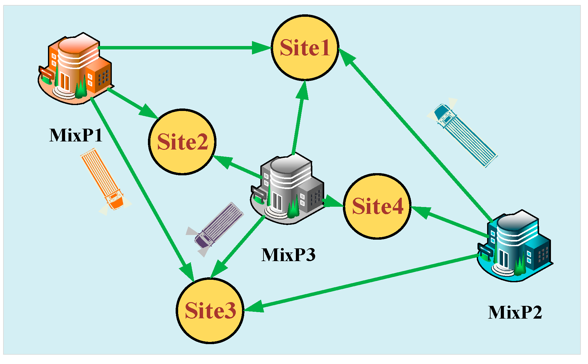
Figure 1. Concrete distribution.
Applsci 13 09256 g001
Figure 2. Overall percentage of evolutionary computation in reviewed articles.
Applsci 13 09256 g002
Figure 3. The flowchart of the improved genetic algorithm (IGA).
Applsci 13 09256 g003
Figure 4. Example of coding operations.
Applsci 13 09256 g004
Figure 5. The crossover of the second layer of coding.
Applsci 13 09256 g005
Figure 6. Mutation in the first layer of coding.
Applsci 13 09256 g006
Figure 7. The optimal path of each algorithm.
Applsci 13 09256 g007
Figure 8. Experiment results.
Applsci 13 09256 g008
Figure 9. Algorithm iteration curve.
Applsci 13 09256 g009
Figure 10. Distribution of the three concrete-mixing plants.
Applsci 13 09256 g010
Table 1. Comparison of research methods and objectives for VRP.
ReferencesContributionsAlgorithmsDisadvantages
[8]The algorithm is improved to solve the GVRP problem.MAThe universality of the algorithm is difficult to guarantee.
[10]The GVRP model was established with the aim of minimizing total fuel consumption by considering some factors that affect vehicle fuel consumption.ACOThe effect of road slope on fuel consumption was not considered.
[11]A multi-objective MDVRP model was established with the aim of minimizing vehicle carbon emission.GAOther factors affecting vehicle fuel consumption are not considered.
[12]A multi-objective MDVRP model was established considering the carbon emission cost and driving time.ACOThe load of the vehicle was not taken into account.
[14]The GVRP models are classified according to their objective functions./The improved algorithms for solving GVRP are not compared and analyzed.
[19]The factors affecting RMC delivery are analyzed, and a model is established with minimum delivery time as the target.GAThe fuel consumption of the vehicle is not taken into account.
[20]The RMC-scheduling model is established by simulation technology. The capacity of the different tankers was not taken into account.
[21]Aiming at the minimum pouring and waiting time of mixing plant, the vehicle-scheduling model is established.GAThe road congestion problem that may be encountered in the actual distribution of tank cars is ignored.
[22]From the perspective of reducing carbon emission, the TDVRP model is established after considering the factors of vehicle speed, distance, and load.SAA method of estimation is used to predict vehicle fuel consumption.
[23]This paper proposes a general delivery model./The time window of distribution and the problem of vehicle failure in the process of distribution are ignored.
[24]A model is proposed for concrete companies to adjust their plans to reduce production costs./It is not conducive to the solution of the model.
[25]RMC delivery is divided into two parts to reduce the difficulty of solving it./The method of multi-mixing collaborative distribution is not considered.
[26]The RMC distribution model is established from the perspective of multi-mixing plant co-operative distribution.BAThe article acquiesces that the volume of all tank cars is the same without considering different models.
Table 2. Description of symbols.
SymbolParameterSymbolParameter
M The total mass of the vehicle d a Air resistance workmanship distance (km)
g Gravitational constant η motor Engine efficiency
L Travel distance (km) A f Frontal area ( m 2 )
β Driving C d Air resistance coefficient
C r Rolling resistance v r Vehicle speed considering the influence of wind speed
ϕ t Effect of temperature (℉) e v Wind influence factor
d r Rolling resistance work distance (km) ρ f Fuel density (kg/L)
λ s Type of pavement ρ Air density ( kg / m 3 )
C f Fuel calorific value (MJ/kg) T Time (h)
Table 3. Parameter value.
SymbolParameterValue
φ t Effect of temperature (℉)46.4
λ s Type of pavement0.29
η motor Engine efficiency0.4
A f Frontal area ( m 2 ) 3.27
β Driving1
C r Rolling resistance0.01
γ f Fuel efficiency0.395
Table 4. Algorithm parameters and calculation results.
AlgorithmParameterResultConvergence Algebra
GANp = 50 G= 500 Pc = 0.8 Pm = 0.1 1.24 × 10 4 64
DENp = 50 G = 500 F0 = 0.4 CR = 0.1 y z = 1 × 10 6 2.713 × 10 6 53
IANp = 50 G = 500 Pm = 0.7 Nc1 = 10
alfa = 1 belta = 1 detas = 0.2
7.626 × 10 5 26
PSON = 50 G = 500 C1 = C2 = 1.5 w = 0.8 xmax = 20 xmin = 20 vmax = 10 vmin = −10 1.384 × 10 8 31
IGANp = 50 G = 500 Pm1 = 0.01 Pm2 = 0.08 Pc1 = 0.5 Pc2 = 0.8 α = 4     λ = 0.85 1.21 × 10 12 19
Table 5. City co-ordinates.
CityCo-OrdinateCityCo-OrdinateCityCo-OrdinateCityCo-Ordinate
1(1304, 2312)9(3488, 1535)17(4312, 790)25(2788, 1491)
2(3639, 1315)10(3326,1556)18(4386, 570)26(2381, 1676)
3(4177, 2244)11(3238, 1229)19(3007, 1970)27(3715, 1678)
4(3712, 1399)12(4196, 1004)20(2562, 1756)28(3918, 2179)
5(4061, 2370)13(4263, 2931)21(3439, 3201)29(2778, 2826)
6(3780, 2212)14(3429, 1908)22(2935, 3240)30(2370, 2975)
7(3676, 2578)15(3507, 2376)23(3140, 3550)31(1332, 695)
8(4029, 2838)16(3394, 2643)24(2545, 2357)
Table 6. Values of relevant algorithm parameters and optimization results.
AlgorithmParameterResultConvergence
Algebra
GANp = 200 G = 100016,738.34920
ACOM = 50 G = 200 Alpha = 1 Beta = 5 Rho = 0.116,011.77158
IANp = 200 G = 1000 Nc1 = 1015,914.02680
TSG = 1000 TabuL = 22 Ca = 20016,976.38780
IGANp = 200 G = 500 Pm1 = 0.02 Pm2 = 0.07 Pc1 = 0.4 Pc2 = 0.7 α = 18     λ = 0.93 15,609.47132
Table 7. Truck configuration of mixing plants.
Mixing plantAB
Truck123456
Total weight (t)39.52739.518.639.539.5
Mixing plantBC
Truck789101112
Total weigh (t)18.6272718.639.527
Table 8. Mixing plants and sites.
Mixing PlantABC
Site 1Distances (km)201514
Time (h)0.470.210.38
Site 2Distances (km)383025
Time (h)0.660.750.4
Site 3Distances (km)154035
Time (h)0.510.850.76
Site 4Distances (km)232045
Time (h)0.570.350.8
Table 9. Four factors with four levels.
NO. α p c p m λ
140.550.030.8
280.60.040.85
3120.650.050.9
4160.70.060.95
Table 10. L 16 ( 4 4 ) orthogonal experimental array.
NO. α p c p m λ CA CA Mv FC FC Mv
11111215.000.195235.0000.872
21222248.001.000230.0000.744
31333216.000.220232.0000.795
41444233.000.634240.0001.000
52123217.000.244219.0000.462
62214229.000.537240.0001.000
72341220.000.317220.0000.487
82432215.000.195208.0000.179
93134207.000.000218.0000.436
103243235.000.683201.0000.000
113312233.000.634214.0000.333
123421229.000.537230.0000.744
134142217.000.244205.0000.103
144231236.000.707224.0000.590
154324241.000.829227.0000.667
164413232.000.610223.0000.564
Table 11. Range analyses.
NO. A :   α B :   p c C :   p m D :   λ CV
140.550.030.80.669
240.60.040.850.821
340.650.050.90.622
440.70.060.950.890
580.550.040.90.396
680.60.030.950.861
780.650.060.80.436
880.70.050.850.184
9120.550.050.950.305
10120.60.060.90.205
11120.650.030.850.424
12120.70.040.80.681
13160.550.060.850.145
14160.60.050.80.625
15160.650.040.950.715
16160.70.030.90.578
k1j3.002 1.515 2.531 2.411
k2j1.878 2.511 2.614 1.573
k3j1.615 2.197 1.737 1.801
K4j2.063 2.334 1.676 2.772
Rj1.387 0.996 0.937 1.199
Table 12. Vehicle-scheduling scheme.
Truck243157
Site334324
Truck861011912
Site142111
Table 13. Comparison of vehicle distribution routes.
SchemeDistribution RouteTotal PathConcrete VolumeFuel Consumption
Original2→1, 4→4, 3→3, 1→178km156 (m3)270 (L)
5→2, 7→1, 8→1, 6→480 km
10→2, 11→4, 9→3, 12→3140 km
GA2→3, 4→3, 3→1, 1→170 km156 (m3)253.5 (L)
5→4, 7→3, 8→4, 6→4100 km
10→1, 11→12, 9→1,12→278 km
IGA2→3, 4→3, 3→4, 1→368 km156 (m3)189.6 (L)
5→2, 7→4, 8→1, 6→485 km
10→2, 11→1, 9→1, 12→167 km
Disclaimer/Publisher’s Note: The statements, opinions and data contained in all publications are solely those of the individual author(s) and contributor(s) and not of MDPI and/or the editor(s). MDPI and/or the editor(s) disclaim responsibility for any injury to people or property resulting from any ideas, methods, instructions or products referred to in the content.