Article

Hyperspectral Image Dimensionality Reduction Algorithm Based on Spatial–Spectral Adaptive Multiple Manifolds

1
Information Department, Hohai University, Nanjing 211100, China
2
Key Laboratory of Water Big Data Technology of Ministry of Water Resources, Hohai University, Nanjing 211100, China
*
Author to whom correspondence should be addressed.
Appl. Sci. 2023, 13(16), 9180; https://doi.org/10.3390/app13169180
Submission received: 30 June 2023 / Revised: 4 August 2023 / Accepted: 10 August 2023 / Published: 11 August 2023
(This article belongs to the Special Issue Advances in Deep Learning for Hyperspectral Image Processing)

Abstract

:
Hyperspectral images contain rich spatial–spectral information and have high dimensions, which can lead to challenges related to feature extraction for classification tasks, resulting in suboptimal performance. We propose a hyperspectral image dimensionality reduction algorithm based on spatial–spectral adaptive multiple manifolds to address the problem of small differences between features of dissimilar samples in the subspace caused by the uniform projection transformation in traditional dimensionality reduction methods. Firstly, to address spatial boundary mismatch problems caused by re-characterizing a pixel using pixels in a fixed area around it as its near neighbors in traditional algorithms, an adaptive weight representation method based on super-pixel segmentation is proposed, which enhances the similarity of similar samples and the dissimilarity of dissimilar samples. Secondly, to address the problem that a single manifold cannot completely characterize the near neighbor between samples of different categories, an adaptive multi-manifold representation method is proposed. The feature representation of the entire hyperspectral data in the low-dimensional subspace is obtained by adaptively fusing the intra- and inter-manifold maps constructed for each category of samples in the spatial and spectral dimensions. Experimental results on two public datasets show that the proposed method achieves better results when performing the hyperspectral image dimensionality reduction task.

1. Introduction

A hyperspectral image (HSI) is a three-dimensional cubic structure with high spectral resolution, which occupies a prominent position in the remote sensing earth observation system [1]. HSIs are widely used in ground–object classification [2,3,4], change detection [5,6], anomaly detection [7,8,9], target detection [10], spectral unmixing [11], etc.
With the development of hyperspectral imaging technology, the increasing number of bands and high spatial resolution pose challenges regarding feature detection and classification [12]. The existing research shows that only a few of the numerous bands contain key information [13]. HSI dimensionality reduction is a solution that reduces the number of dimensions in HSIs through a series of transformations while retaining effective feature information, considering both spatial and spectral data [14]. Feature extraction that finds the corresponding projection matrix according to linear or non-linear transformation and projects the original HSI data from a high-dimensional spectral feature space to a subspace of lower dimensionality via matrix transformation is one of the effective dimensionality reduction approaches [15]. A linear transformation is the most widely used dimensionality reduction method in the early stage, as it generally achieves dimensionality reduction via a linear transformation of spectral feature information. Principal component analysis (PCA) [16], independent component analysis (ICA) [17], and linear discriminant analysis (LDA) [18] are based on linear transformations of the data. This idea means that the projection from the original space to the lower-dimensional subspace involves linear combinations of the input features with fixed coefficients. These dimensionality reduction methods have achieved good effects to some extent. But since the features of HSIs are not linearly distributed, using such feature extraction methods will limit the subsequent classification performance.
Therefore, the manifold learning method based on graph embedding (GE) is applied to the dimensionality reduction task of HSIs. It effectively improves the dimensionality reduction as a non-linear feature extraction method. Yan [19] et al. proposed a graph embedding framework to describe the dimensionality reduction methods used in a unified manner. To further enhance the dimensionality reduction effect, Luo [20] et al. proposed a supervised local geometric structure Fisher analysis (LGSFA) algorithm. The algorithm constructs graphs using labeled samples to improve the synergy of same-category data and reconstructed data and enhance the separation of dissimilar data and reconstructed data. However, the disadvantage of this method is that it can destroy the overall structure of the manifold in low-dimensional space. To better portray the local reconstruction relationships between data, He et al. [21] proposed the subspace manifold learning algorithm based on neighborhood preserving embedding (NPE), which can better solve the new sample problem by preserving the local near neighbor structure of the original manifold space. Based on the local preservation discriminant analysis, Pu et al. [22] proposed a new spatial–spectral similarity metric that maps the distance between two image blocks in an HSI, which can effectively deal with the redundancy problem caused by the spectral features, as well as the spatial relationship between pixels. Deng et al. [23] proposed a modified tensor locality preserving projection (MTLPP) algorithm, which can improve the effect of noise on the near neighbor graph by constructing the neighbor graph on the pairwise feature space instead of the original space. But the algorithm does not work for points distributed at the category boundaries, which limits the improvement in the dimensionality reduction performance to some extent. To improve this problem, several sparse representation methods have emerged in the field of signal processing in recent years. Moreover, sparse representation methods have been gradually applied to HSI dimensionality reduction, noise reduction, and classification tasks. Cheng et al. [24] proposed the sparsity preserving graph embedding (SPGE) algorithm in which the number of near neighbors can be adaptively adjusted. In the case of fixed dictionaries, SPGE has good robustness to noisy data. Therefore, its dimensionality reduction effect is somewhat improved. However, HSI datasets are composed of different ground object categories. Each category of ground object has common features belonging to it and unique features that distinguish it from other categories. Theoretically, different classes of ground objects should all be located on different smooth low-dimensional sub-manifolds. Therefore, the above algorithms that use single-manifolds to construct graphs cannot reveal the multi-manifold structure of hyperspectral data, thus limiting the improvement in dimensionality reduction performance.
To explore the intrinsic multi-manifold structure of high-dimensional data, multi-manifold learning methods have become a focus of scholars’ research. Wang [25] et al. proposed a multi-manifold learning algorithm based on multi-linear local and global preserving embedding (MLGPE) by maintaining global–local near-neighbor features within each class data. The algorithm separately performs feature learning for each sub-manifold and then projects the data onto the different sub-manifold into the relevant low-dimensional space. To address the problem of multi-feature fusion and dimension reduction in HSIs, Huang et al. [26] proposed a multi-feature manifold learning method based on spectral-texture features, which significantly improved the classification accuracy of HSI ground objects. It is useful for exploring efficient feature fusion methods. Compared to single-manifold learning methods, although the above feature extraction methods based on multi-manifold show strong performance in image classification tasks, they only seek low-dimensional representations of high-dimensional data from spectral feature information. They did not utilize the rich spatial near-neighbor information of HSIs, which significantly limits the improvement in classification performance of the images after dimensionality reduction.
In recent years, many studies have shown that the rational use of spatial information is an effective way to improve the classification accuracy of an HSI. Thus, various dimensionality reduction methods based on space–spectrum strategies have emerged. Li et al. [27] proposed a cooperative representation algorithm based on multi-task learning for the classification tasks. Kang [28] et al. proposed a fast HSI space–spectrum reduction technique based on edge-preserving filtering, which has the advantage of fast reduction speed and largely reduces the computational complexity of the traditional space–spectrum reduction algorithms. In addition, super-pixels can group pixels using the similarity of features between pixels. Using a small number of super-pixels instead of a large number of pixels to express image features can effectively reduce the complexity of image processing. Therefore, super-pixels are gradually used in dimensionality reduction methods based on spatial–spectral strategies. Zhang et al. [29] proposed a multiscale super-pixel-based sparse representation (MSSR) algorithm for HSI classification. The algorithm achieved good classification results using the joint sparse representation to classify the obtained multiscale super-pixels. Liu et al. [30] proposed a super-pixel-wise collaborative-representation graph embedding (SPCRGE) algorithm, which computed the global projection matrix in low-dimensional space by reducing the differences between pixels in a single super-pixel block while increasing the differences between images with different super-pixels, thus achieving a good dimensionality reduction effect. Dong et al. [31] proposed a new spatial–spectral manifold distance (SSMD) to improve the metric learning performance in HSI dimensionality reduction and classification by maintaining the integrity of the constructed manifolds. SSMD achieves good dimensionality reduction performance by selecting appropriate adjacent points in labeled and unlabeled data to construct manifolds with spatial–spectral information.
In the current research into HSI dimensionality reduction methods, the following problems still exist:
(1) The limited dimensionality reduction strategy based on multi-manifold learning hardly captures the intrinsic variations and discriminative features present in different classes within the data, which results from the poor representational power of HSIs.
(2) When using spatial information, traditional dimensionality reduction methods often select the pixels located in a fixed window size region around a pixel as the near neighbors to find the spectral feature value of the central pixel. However, this strategy tends to set the same weights for all pixels in the fixed region and may be unable to identify and focus on the most informative features, thus losing essential information of his, such as boundary.
Based on this observation, we propose an HSI dimensionality reduction algorithm based on spatial–spectral adaptive multi-manifold analysis (SSAMMA). The algorithm consists of two main modules: the super-pixel-based adaptive weight representation module (SAWRM) and the spatial–spectral multi-manifold module (SSMMM). SAWRM first performs super-pixel representation of HSIs via the image segmentation algorithm. Then, an adaptive weighted representation of the samples in each super-pixel block is performed. SSMMM constructs a multi-manifold map for the new image. By adaptively fusing the intra- and inter-manifold maps constructed for each category of samples in the spatial and spectral dimensions, the spatial–spectral intra-manifold maps and spatial–spectral inter-manifold maps on each sub-manifold map are obtained, meaning that the projection matrix corresponding to each sub-manifold is found. We aim to provide an alternative way to construct multi-manifold graphs, thus obtaining a new representation of HIS. The proposed method is able to improve the accuracy of classification. The experimental results using two public datasets show that the method achieves good dimensionality reduction results.
The rest of the paper is organized as follows: Section 2 introduces the related work, including the super-pixel segmentation algorithm and the dimensionality reduction algorithm based on manifold learning; Section 3 introduces the proposed method SSAMMA, which consists of SAWRM and SSMMM; Section 4 performs experimental validation of the proposed method using two datasets and analyzes the experimental results to evaluate the dimensionality reduction performance of the model; and Section 5 summarizes the contents of the paper.

2. Related Work

2.1. Super-Pixel Segmentation Algorithm

Simple linear iterative clustering (SLIC) [32] is the most widely used super-pixel segmentation algorithm. The advantage of super-pixels is that a small number of super-pixels can be used to express image features instead of a large number of homogeneous pixels while reducing the complexity of image processing [33]. The super-pixel image blocks obtained via super-pixel segmentation generally not only compromise the boundary information of the objects in the image, but also retain the effective feature information for subsequent intelligent image processing. Therefore, the super-pixel image blocks are suitable for HSI classification and segmentation tasks.
The main algorithmic steps are as follows [34]:
(1) Dimensionality reduction in HSI data: PCA is used to downscale the hyperspectral data to three dimensions. The first three principal components are used to generate false color images.
(2) Cluster center initialization: If N pixels are pre-segmented into K super-pixels of the same size, each super-pixel has N / K pixels. The distance between adjacent clustering centers is obtained via S = N / K . The clustering centers are uniformly set in the original image based on the number of super-pixels.
(3) Re-optimize the clustering centers: The gradient values of all pixels in the n × n neighborhood are calculated. The seed points are moved to the lowest gradient, thus preventing the seed points from falling on the boundaries with large gradients.
(4) Determine the clustering center of each pixel in the domain formed by each clustering center: to accelerate the convergence of the algorithm, the search range of the algorithm is set at 2 S × 2 S .
(5) Distance metric: we calculate the color distance d c and spatial distance d s of each pixel to the cluster center to obtain the final distance metric D , using the following equation.
D = ( d c N c ) 2 + ( d s N s ) 2
N s is the maximum spatial distance within the class. N s = S = N / K . N c changes with the image. It indicates the maximum color distance, and its default is taken as 10. After that point, the seed point with the shortest distance from each pixel is taken as the cluster center of that point.
(6) Iterative optimization: we keep iterating the above steps until the clustering center of each pixel no longer changes. It is found that after 10 iterations, most of the images can achieve more satisfactory results, meaning that the number of iterations is usually set to 10.

2.2. Dimensionality Reduction Algorithm Based on Manifold Learning

In recent years, manifold learning has discovered potential manifolds in high-dimensional data to achieve better dimensionality reduction. Several scholars have proposed manifold learning algorithms based on graph embedding to achieve dimensionality reduction. Manifold learning has been a research hotspot in the field of machine learning and artificial intelligence. It has an important application in the field of non-linear dimensionality reduction algorithms. Manifold learning takes advantage of the concept that local and Euclidean spaces are isomorphic spaces that embed high-dimensional data spaces into low-dimensional manifold structures, thus representing high-dimensional data structures with low-dimensional local Euclidean features. The mathematical description of manifold learning can be expressed as follows: The dataset to be observed is assumed to be X = [ x 1 , x 2 , , x N ] R D × N . D is the number of original bands. N is the total number of samples. Sample labels are described as l i { 1 , 2 , , c } , and c is the total number of categories. The data set is described in the low-dimensional space as being Z = [ z 1 , z 2 , , z N ] R d × N , and d (d ≪ D) is the number of bands after dimensionality reduction. The purpose of manifold learning is to find a mapping f , such that Z = f ( X ) , by maintaining some relationship between the samples.

3. Proposed Method

Taking the IP dataset as an example, the overall framework of the proposed SSAMMA is shown in Figure 1. The basic process was as follows. Firstly, the SLIC algorithm was used to segment the HSI to obtain k adaptively sized super-pixel image blocks { S 1 , S 2 , , S k } . The samples in the spatial region block were adaptively weighted in each image block to obtain a new image to show that samples of the same category had more similar spectral lines. Secondly, the HSIs were randomly divided into training samples and test samples. For each category of ground objects in the training samples, a single-manifold map was constructed. The optimal mapping matrix for each sub-manifold was found by combining the spatial–spectral intra-manifold map and the spatial–spectral inter-manifold map. Finally, the pixels in each sub-manifold are downscaled. The feature representation of the entire hyperspectral data in the low-dimensional subspace is obtained by combining all of the sample features in the low-dimensional subspace. The obtained low-dimensional data cube is fed into the classifier to obtain the final classification results.

3.1. Regional Adaptive Weight Representation

Pixels in HSIs that are spatially close to each other usually belong to the same category of ground objects. In practice, due to complex geographical and climatic conditions, ground objects in the same category may exhibit different spectral characteristics, and ground objects in different categories may exhibit the same spectral characteristics. This issue means that the features of the pixel’s own spectrum do not fully reflect the unique feature information of the category to which it belongs. Considering the spatial significance of pixels, the spectral information of spatially neighbor points can be used to compensate for the shortage of its own spectrum, which does not fully reflect the category information. This approach not only makes the spectral features of similar features more similar, but also makes the spectral differences between dissimilar pixels increase. The conventional algorithm generally uses the average weight of fixed neighborhood pixels as the spectral feature value of the pixels, which has the following disadvantages: The fixed near-neighbor region is not suitable for pixels on the boundary of spatially dissimilar ground objects. The calculation of weights in the fixed region is not adaptively adjusted according to the distance from the central pixel. Thus, pixels further from the center pixel and pixels closer to it are given the same weight, resulting in ineffective use of spatial information. In view of this issue, an improved region adaptive weight representation method was proposed in this study that uses the super-pixel segmentation technique, which is expressed as follows. The SLIC algorithm was used to segment the HSI to obtain k adaptively sized super-pixel image blocks { S 1 , S 2 , , S k } . The pixels in any image block S i after segmentation were represented as { x 1 , x 2 , , x N i } , where N i is the total number of pixels in the i pixel block. For any pixel x i in any pixel block, its pixel value x i after regional adaptive weight representation could be expressed via Equation (2).
x i = j = 1 N i 1 w i j x j N i 1 + γ x i
where γ is the real parameter, and the adaptive weight w i j is the weight representation between pixel points x i and x j . We supposed that the spatial coordinates of two pixels x and y are denoted as ( a , b ) and ( c , d ) , respectively. The pixel values are denoted as x i , y i . Then, w i j can be expressed via Equation (3).
w i j = ( 1 λ ) d i j + λ S i j
where d i j is the Euclidean distance between the spatial coordinates of two pixels x and y , i.e., d i j = ( a c ) 2 + ( b d ) 2 . The choice of λ depends on the specific application and the data characteristics. S i j denotes the cosine similarity of the spectral features between two pixels x and y , i.e., S i j = i = 1 N i x i y i / i = 1 N i x i 2 i = 1 N i y i 2 .

3.2. Space–Spectrum Adaptive Multi-Manifold Analysis

A new image was obtained after a regionally adaptive weight representation of each pixel in the image was performed. The spectral curves of pixels of the same category in the new image were more similar. Then, c manifold graphs were constructed for each class of ground objects in the new image to find the low-dimensional feature representation of each class of ground object, where c denotes the number of the classes of ground object in the image. Supervised multi-manifold learning (SMML) can reduce the dimensionality of data by constructing multi-manifold graphs. However, SMML only considers inter-class relationships between HSI data and does not take intra-class relationships into account. In view of this, we proposed a spatial–spectral adaptive multi-manifold analysis method. The steps of the algorithm were as follows. Firstly, the new image obtained from the adaptive weight representation of the region was divided into different subsets according to the class labels of the samples. Each subset was a separate sub-manifold. The intra- and the inter-manifold maps were constructed in the spatial and spectral dimensions of each sub-manifold. By adaptively fusing the intra- and inter-manifold maps constructed for each sub-manifold in the spatial and spectral dimensions, the spatial–spectral intra-manifold maps and spatial–spectral inter-manifold maps on each sub-manifold map were obtained, meaning that the projection matrix corresponding to each sub-manifold was found. Finally, the pixels in each sub-manifold were downscaled. The features of all samples in the low-dimensional subspace were combined to obtain the feature representation of the entire hyperspectral data in the low-dimensional subspace. Based on this approach, the spatial–spectral adaptive graph embedding algorithm effectively fused the low-dimensional embedding of each sample point in each sub-manifold and used it to perform classification, thus achieving a better classification result.
In the HSI spectral dimension, the set of ground objects in each category was considered to be a sub-manifold. We assumed that the i pixel on the r manifold was represented as M r i . The set of pixels on the r sub-manifold can be denoted as { M r 1 , M r 2 , , M r n r } , where n r is the total number of samples in category r . Firstly, based on the spectral similarity relationship between the samples, the set of intra-manifold near neighbors N i n and the set of inter-manifold nearest neighbors N o u t for each pixel of each sub-manifold in the spectral dimension could be obtained. We assumed that V 1 , V 2 , , V c denotes the projection matrix of c in different sub-manifolds of the high-dimensional data, where c is the number of classes of the high-dimensional data. In the spectral dimension, in order to minimize the aggregation of intra-manifold data and maximize the separation of inter-manifold data in the low-dimensional space, the optimization problem can be expressed via Equation (4) [35].
J V 1 , V 2 , , V c max ( V 1 , V 2 , , V c ) = J 1 ( V 1 , V 2 , , V c ) J 2 ( V 1 , V 2 , , V c ) = r = 1 c ( i = 1 n r p = 1 k 1 | | V r T M r i V r T M r p | | 2 A r i p ) r = 1 c ( i = 1 n r q = 1 k 2 | | V r T M r i V r T M r q | | 2 B r i q )
where J V 1 , V 2 , , V c max ( V 1 , V 2 , , V c ) denotes the objective function used to minimize the aggregation of intra-manifold data and maximize the separation of inter-manifold data. J 1 ( V 1 , V 2 , , V c ) denotes the objective function used to maximize the separation of inter-manifold data, and J 2 ( V 1 , V 2 , , V c ) denotes the objective function used to minimize the aggregation of intra-manifold data. M r p denotes p as a inter-manifold near neighbor of M r i . M r q denotes q as a intra-manifold near neighbor of M r i . k 1 and k 2 denote the number of inter- and intra-manifold near neighbors. A r i p denotes the weight matrix for the similarity between M r i and its inter-manifold near neighbor. B r i q denotes the weight matrix for the similarity between M r i and its intra-manifold near neighbor. They are defined via Equations (5) and (6).
A r i p = e x p ( | | M r i M r p | | / σ 2 )
B r i p = e x p ( | | M r i M r q | | / σ 2 )
where σ is the heat kernel. This algorithm iterates to find the projection matrix on the c sub-manifold. For the i manifold, the objective function is expressed as shown in Equation (7).
J V r max ( V r ) = ( J 1 ( V r ) + F 1 ) ( J 2 ( V r ) + F 2 ) = ( i = 1 n r p = 1 k 1 | | V r T M r i V r T M r p | | 2 A r i p + F 1 ) ( i = 1 n r q = 1 k 2 | | V r T M r i V r T M r q | | 2 B r i q + F 2 )
where F 1 and F 2 are two constant matrices that can be neglected in the process of computation of V r , meaning that Equation (8) can be obtained.
J 1 ( V r ) = i = 1 n r p = 1 k 1 | | V r T M r i V r T M r p | | 2 A r i p = i = 1 n r p = 1 k 1 tr ( ( V r T M r i V r T M r p ) ( V r T M r i V r T M r p ) T A r i p ) = i = 1 n r p = 1 k 1 tr ( V r T [ ( M r i M r p ) ( M r i M r p ) T A r i p ] V r ) = tr ( V r T i = 1 n r p = 1 k 1 [ ( M r i M r p ) ( M r i M r p ) T A r i p ] V r ) = tr ( V r T Q 1 r V r )
where Q 1 r = ( M r i M r p ) ( M r i M r p ) T A r i p .
J 2 ( V r ) = i = 1 n r q = 1 k 1 V r T M r i V r T M r q 2 B r i q = tr ( V r T Q 2 r V r )
Thus, in the spectral dimension, Equation (10) can be obtained.
J V 1 , V 2 , , V c m a x ( V 1 , V 2 , , V c )
The above equation can be translated into Equation (11).
( Q 1 r Q 2 r ) V r = λ r V r
In the HSI space dimension, if the pixel x i is located on the r spectral sub-manifold, it can be represented as M r i . Since the pixels in the local spatial pixel block in which x i is located are located on the same spatial sub-manifold as x i , the neighboring pixels of x i can be represented as M r i 1 , M r i 2 , M r i m , M r i k where k is the total number of spatial neighbors. For any spatial sub-manifold M r , we assumed that the i pixel on the r manifold is represented as M r i . The set of pixels on the r sub-manifold can be represented as { M r 1 , M r 2 , M r n r } . n r is the total number of samples in the r class. In the manifold intra-graph, the weighted scatter matrix of this spatial block within the manifold can be represented as follows:
S r w = i = 1 n r m = 1 k w m j = 1 k w j ( M r i M r i m ) ( M r i M r i m ) T
where w m is the weight between the nearest neighbor image element M r i m and the central image element M r i , which is defined as follows:
w m = exp { γ | | M r i M r i m | | 2 }
In the inter-manifold graph, the scatter matrixes from vertex M r i to submanifold M s ( s r ) and from vertex M s j to submanifold M r can be defined via Equations (14) and (15).
H 1 ( M r i , M s ) = i = 1 n s m = 1 k w m j = 1 k w j ( M r i M s i m ) ( M r i M s i m ) T
H 2 ( M s j , M r ) = t = 1 n r m = 1 k w m p = 1 k w p ( M r t m M s j ) ( M r t m M s j ) T
Therefore, the inter-class scatter matrix between sub-manifold M r i and sub-manifold M s ( s r ) can be represented via Equation (16).
H ( M r , M s ) = i = 1 n r H 1 ( M r i , M s ) + i = 1 n s H 2 ( M s j , M r )
The scatter matrix between sub-manifold M r and all other sub-manifolds can be calculated via Equation (17).
H r b = s = 1 , s r c H ( M r , M s )
The objective function of sub-manifold M r in the manifold intra-graph can be represented by Equation (18).
J w ( V r ) = tr ( V r T S r w V r )
The objective function of sub-manifold M r in the inter-manifold graph can be represented by Equation (19):
J b ( V r ) = tr ( V r T H r b V r )
To increase the aggregation of spatial neighborhood data features in each manifold and make the features of data between manifolds as distinguishable as possible, the condition shown in Equation (20) must be satisfied in each manifold space.
J ( V r ) = argmax J b ( V r ) J w ( V r ) = max tr ( V r T H r b V r ) V r T S r w V r
Using the Lagrange multiplier method, the optimization problem in Equation (20) can be transformed into Equation (21).
H r b V r = λ r S r w V r
In HSIs, the spectral reflection characteristics between different categories of objects were represented by spectral information, and the feature information on the spatial dimension reflected the spatial distribution of objects. Combining spectral and spatial information of HSIs for feature extraction could further improve the performance of dimensionality reduction. Therefore, this study proposed a dimensionality reduction algorithm based on SSAMMA. The algorithm extracted feature information from HSIs in both spatial and spectral dimensions and gradually obtained the intra- and inter-manifold scatter matrixes of each submanifold M r . By combining spatial and spectral information, the multi-manifold structure in hyperspectral data could be effectively revealed.
The intra-manifold scatter matrix of submanifold M r could be represented by Equation (21), and the inter-manifold scatter matrix could be represented by Equation (22).
( Q 1 r Q 2 r ) V r = λ r V r
Combining the two equations, we can find Equation (23).
[ α H r b + β ( Q 1 r Q 2 r ) ] V r = λ r ( α S r w + β ) V r
where α and β are parameters that balance spectral and spatial information, λ r is the eigenvalue in Equation (23), and the d eigenvectors corresponding to the d eigenvalues arranged from large to small can be obtained. The best projection matrix is composed of these eigenvectors, that is, V r = [ V r 1 , V r 2 , , V r d ] .
For c sub-manifolds, c projection matrices V 1 , V 2 , , V c can, in turn, be obtained. If the low-dimensional embedding of X in each sub-manifold is Y 1 = V 1 T X , Y 2 = V 2 T X , , Y c = V c T X , the final low-dimensional embedding of fusing different sub-manifolds can be obtained, and the final low-dimensional embedding Y can be represented by Y = [ Y 1 , Y 2 , Y c ] .

4. Experimental Results and Analysis

4.1. Datasets

To verify the effectiveness of the proposed SSAMMA, we used two benchmark datasets in our related experiments: Indian Pines (IP) and the University of Pavia (UP).
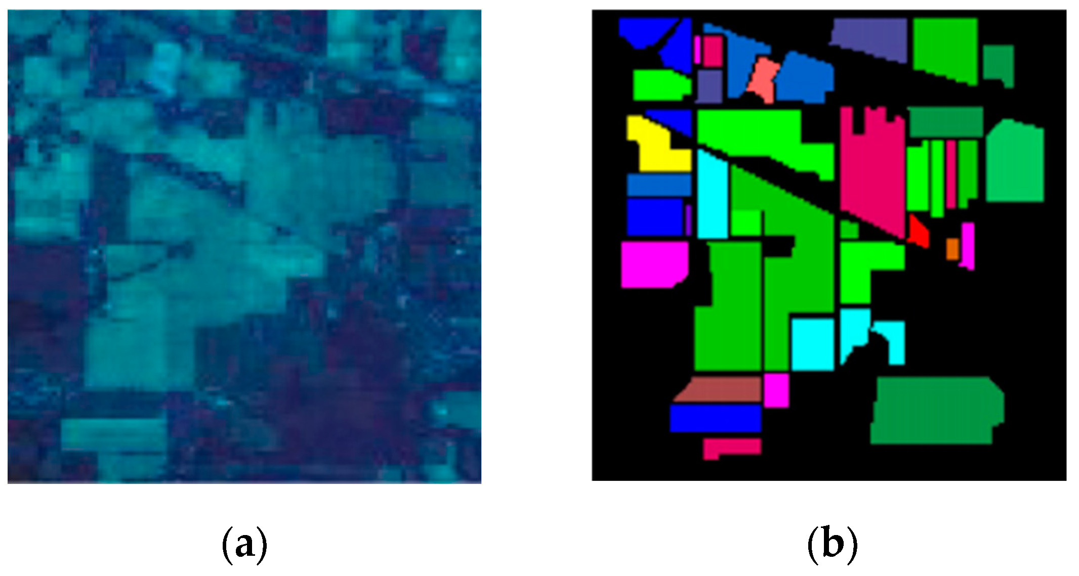
In 1992, the AVIRIS sensor obtained an IP dataset by photographing agricultural areas in Northwest Indiana. This dataset has a spectral wavelength range of 0.4–2.45 μm, a spatial resolution of 20 m, and 16 feature classes. The dataset size is 145 × 145 pixels, including 220 bands. After excluding 20 bands with severe water absorption, the remaining 200 bands WERE used as the study objects. Figure 2 shows the false-color composite image and the ground-truth map of the IP dataset. Table 1 shows the number of each ground object category in this dataset.
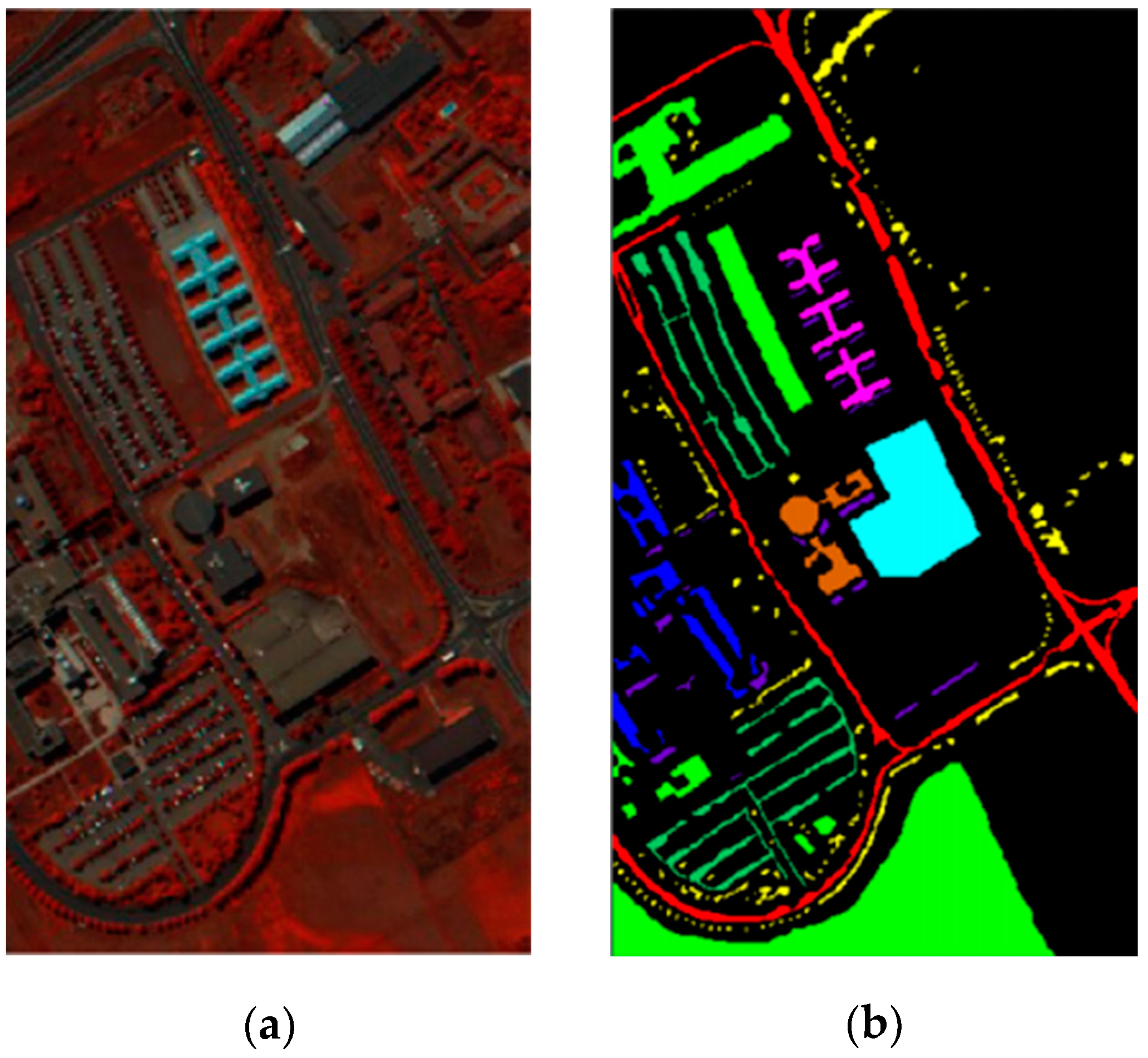
The UP dataset was acquired via the ROSIS sensor at the University of Pavia, Italy, in 2003. It has a spectral range of 0.43–0.86 μm, a spatial resolution of 1.3 m, and 9 feature classes. The dataset has a size of 610 × 340 and includes 115 bands. After removing 12 noisy bands, the remaining 103 bands were used as the objects of study. Figure 3 shows the false-color composite image and ground-truth map of the UP dataset. The ground objects of the UP dataset are shown in Table 2.

4.2. Implementation Details

During the experiments, the samples of the two datasets were randomly divided into a training dataset and a test dataset. The training dataset was used to train the proposed model SSAMMA to obtain the best projection matrix. The test dataset was used to verify the effectiveness of the proposed model SSAMMA for dimensionality reduction. To reduce the chance, 10 replicate trials were performed under the same set of parameters. The effect of the algorithm under this set of parameters was expressed by calculating the average result of the 10 replicate trials. In addition, to quantitatively evaluate the effectiveness of the proposed method, the classification result graph, overall accuracy (OA), average accuracy (AA), and kappa coefficient (Kappa) were used as evaluation metrics.

4.3. Comparison with Existing Methods

The comparison algorithms include PCA [16], LPP [23], MMDA [35], NSPE [36], MFA [37], MLE [38], SPCA [39], and SSMRPE [40]. PCA adopts the principle of maximizing the global data variance to find the orthogonal projection. The main purpose of LPP is to find a linear transformation of the data that minimizes the distortion of the pairwise relationships between neighboring data points. In other words, LPP tries to map similar data points close to each other in the reduced space. MMDA is a novel discriminative multi-manifold analysis method that learns discriminative features from image patches. NSPE can maintain non-negative sparse reconstruction relations for data in low-dimensional subspaces. MFA based on an extreme learning machine is recommended to improve spectral regression and kernel marginal Fisher analysis. MLE further improves the multi-streamer LE algorithm by adding spatial and data tagging information. SPCA considers the diversity of different homogeneous regions, which means that different regions should have different projections. SPCA is able to make full use of the spatial information through super-pixel segmentation. SSMRPE utilizes a new spatial–spectral combined distance (SSCD) to fuse the spatial structure and spectral information to select effective spatial–spectral neighbors of HSI pixels. Among all of the compared algorithms, PCA, LPP, MFA, NSPE, MLE, and MMDA are dimensionality reduction methods based on spectral information, which consider only the spectral information of HSIs for the dimensionality reduction task. In addition, among all of the downscaling methods based on spectral information, LPP, MFA, and NSPE are single-manifold learning methods, while MLE and MMDA are multi-manifold learning methods. The SPCA, SSMRPE, and SSAMMA algorithms consider both the spectral information and spatial structure of an HSI. To ensure the accuracy of the comparison experiments, the SVM classifier was used to classify the dimensionality reduction data obtained via the different algorithms.
For better analysis of experimental parameters, the optimal values of their parameters are chosen for all comparison algorithms in the paper. Based on the IP dataset, the number of near neighbors in the LPP, MFA, NSPE, and MLE algorithms is set to 8. The MMDA inter-manifold near neighbor is set at seven and the intra-manifold near neighbor is set at nine. The spatial window size of SPCA is set at eight, and the number of near neighbors is set at nine. The spatial window size of SSMRPE is set at five, and the number of near neighbors is set at nine. Using the PU data set, the number of near neighbors in the LPP, MFA, NSPE, and MLE MFA, NSPE, and MLE is set at nine. The number of inter-manifold near neighbors of MMDA and SPCA is set at 8, and the number of intra-manifold near neighbors is set at 10. The spatial window size of SSMRPE is set at 13, and the number of near neighbors is set at 20. The way that we calculate these optimal numbers is identical to the proposed SSAMMA method. The details can be found in the parameter analysis of this paper.

4.3.1. Classification Results on the IP Dataset

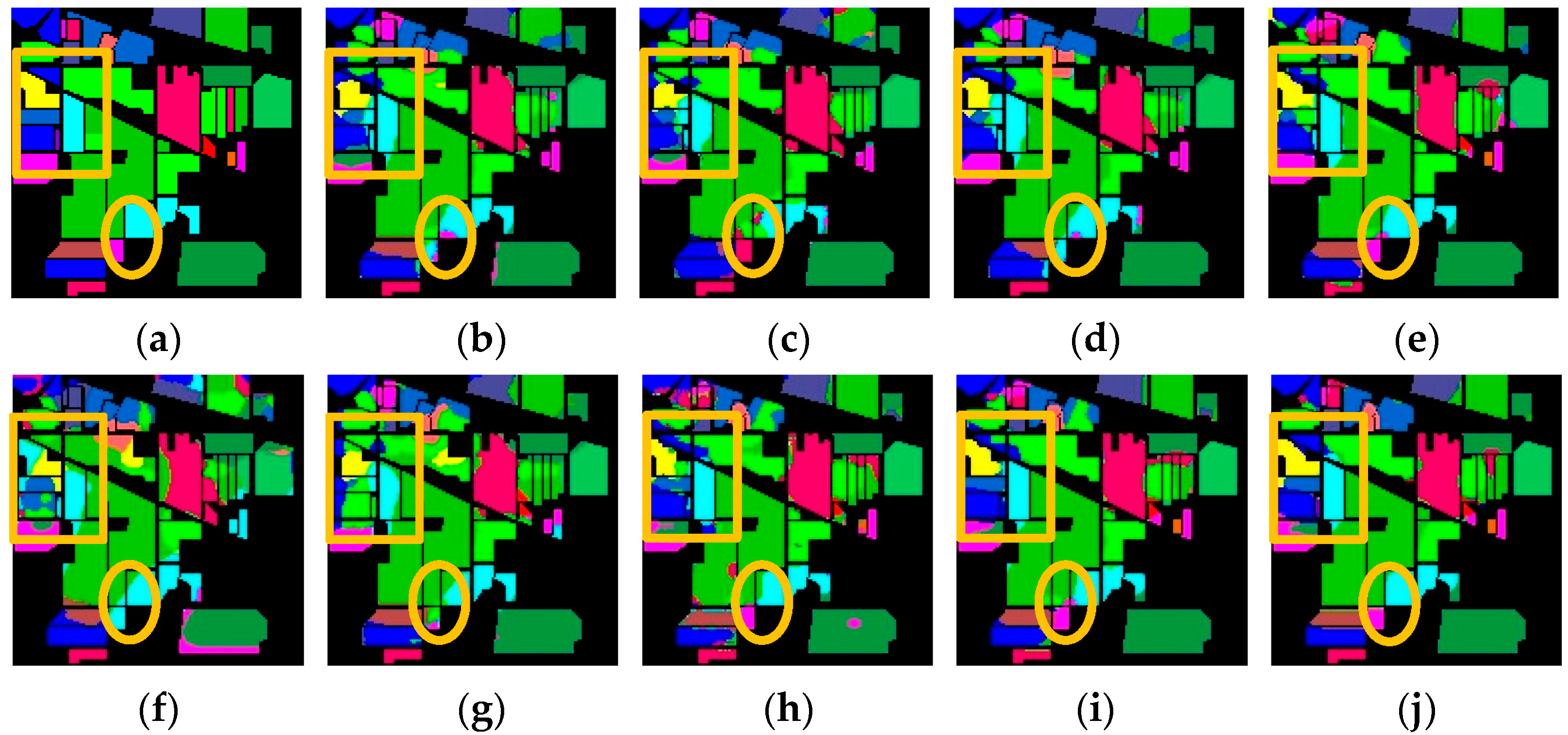
Using the IP dataset, 20 samples of each type of ground object were randomly used as the training set, and the remaining samples were used as the test set. The classification results obtained via the nine dimensionality reduction algorithms are shown in Table 3. Figure 4 visualizes the classification maps obtained via these nine dimensionality reduction algorithms.
In Table 3, it can be seen that when using the IP dataset, the dimensionality reduction effect of the method based on multi-manifold embedding is better than that of the traditional single-manifold algorithm, which proves the correctness of the multi-manifold assumption. Additionally, considering the spatial features of HSIs, the classification performance of the manifold learning algorithm based on the spatial–spectral features is better than that of the manifold learning algorithm that only considers the spectral feature. Among these algorithms, the proposed method achieves the highest classification accuracy, and the OA, AA, and Kappa are 92.87%, 90.26%, and 91.48%, respectively. Compared to SSMRPE, which also considers the spatial–spectral features, the proposed method is improved by 4.12%, 3.89%, and 3.88% in OA, AA, and Kappa. Since the proposed method adaptively fuses the multi-manifold maps of spatial and spectral dimensions, the proposed method more adequately extracts the spatial–spectral features of each class of HSI, thus achieving the best effect. As can be seen in Figure 4, compared to other dimensionality reduction algorithms, the classification result map obtained via the proposed SSAMMA is richer in detail and has the least number of misclassified samples. In contrast, the classification maps obtained via the two-dimensionality reduction algorithms, i.e., NSPE and MLE, have the most misclassified samples and a large amount of noise in the classification result maps. In addition, the classification result map obtained via the algorithm that considers the spatial–spectral features has clearer classification boundaries and better visual effects than the single-manifold learning algorithm and the multi-manifold algorithm that only uses spectral features.

4.3.2. Classification Results on the UP Dataset

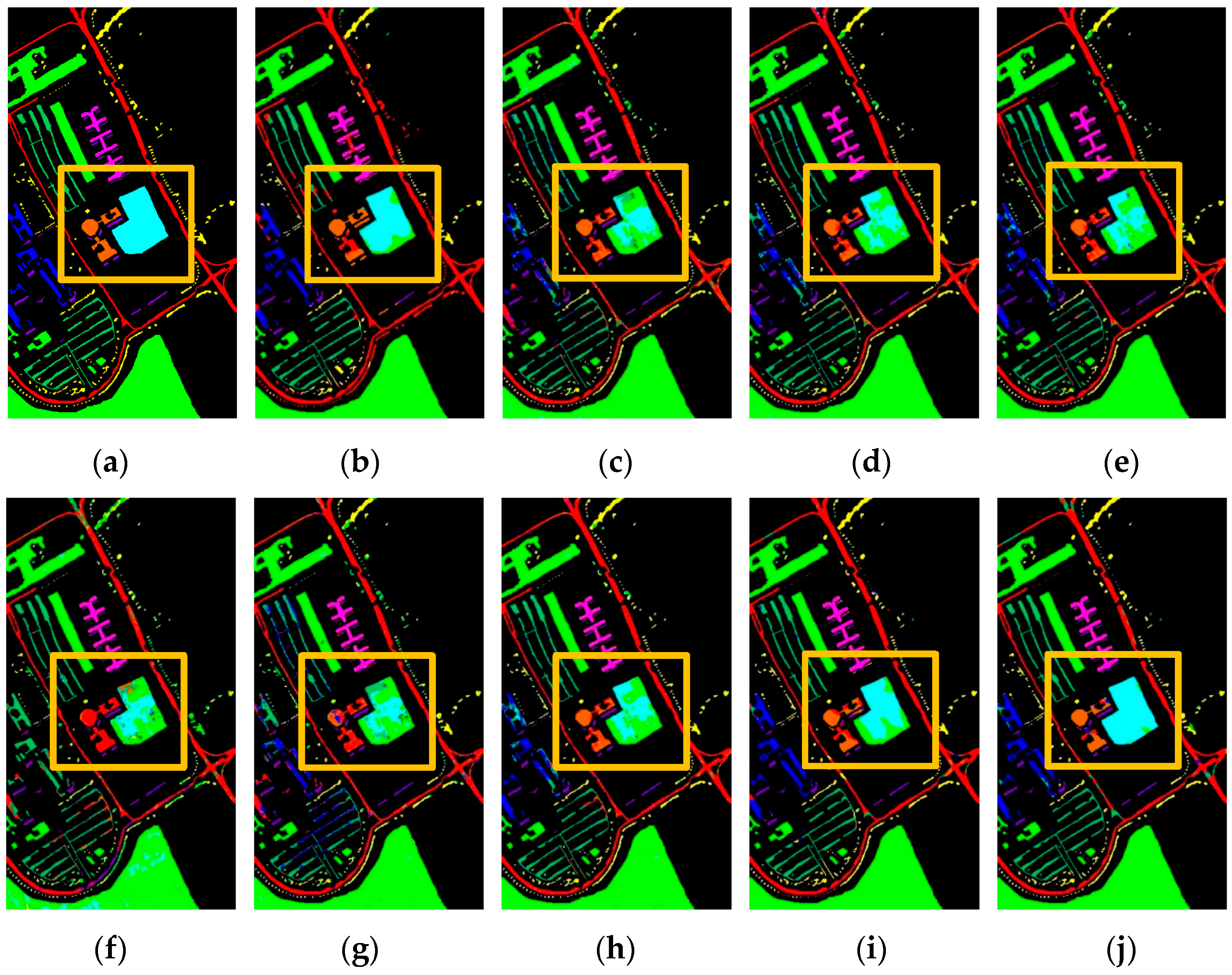
Using the UP dataset, 30 samples of data for each class of features were randomly used as the training set, and the rest of the samples were used as the test set. Accordingly, the classification results obtained via the nine dimensionality reduction algorithms are shown in Table 4. Figure 5 visualizes the classification feature maps obtained via these nine dimensionality reduction algorithms.
As can be seen in Table 4, when using the UP dataset, the dimensionality reduction method based on the multi-manifold feature extraction strategy is more effective at classification than the traditional algorithm. Among these algorithms, the proposed SSAMMA achieves the highest classification accuracy, and the values of OA, AA, and Kappa are 96.53%, 94.12%, and 95.38%, respectively. Compared to SSMRPE, which is also based on spatial–spectral feature extraction, the proposed method improves the OA, AA, and Kappa by 4.18%, 2.93%, and 4.06%, respectively. Since the proposed method fuses the multi-manifold map of spatial and spectral dimensions, it can extract more discriminative features of each type of ground object for the spatial–spectral features of HSIs, thus achieving the highest classification accuracy after the dimensionality reduction. As can be seen in Figure 5, compared to other dimensionality reduction algorithms, the proposed method SSAMMA obtains a more detailed classification result map using the PU data set with the least number of misclassified samples. In contrast, the classification maps obtained via the two-dimensionality reduction algorithms, i.e., NSPE and MLE, have the most misclassified samples and a large amount of noise in the classification result maps. In addition, the classification result maps obtained via the dimensionality reduction algorithm, which consider the spatial–spectral features obtained using the PU dataset, have clearer classification boundaries, and the classification maps have the least noise.

4.4. Parameter Analysis

For better analysis of the parameters, all comparison algorithms in the paper are used for the optimal values of their parameters. The parameter settings of various algorithms have been described in detail in Section 4.2 and are not repeated in this section.

4.4.1. Inter-Manifold and Intra-Manifold near Neighbors a and b

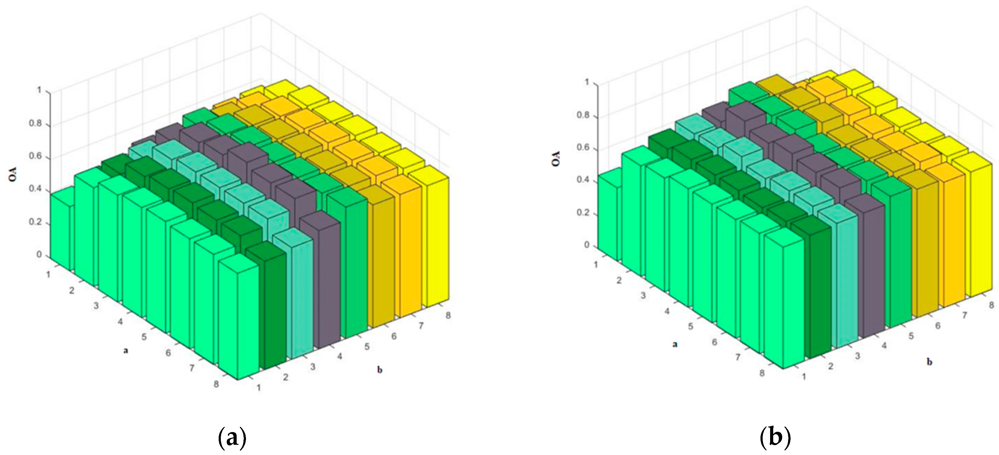
To investigate the influence of inter-manifold near neighbor a and intra-manifold near neighbor b on the final dimensionality reduction effect on the spectral dimensional map, 15 samples are selected as training samples using the IP and PU datasets, and the other samples are used as test samples. The variations in parameters a and b are chosen as {1, 2, …, 8} and {1, 2, …, 8}, respectively. Figure 6 shows the classification results after dimensionality reduction obtained by setting different parameters a and b using the two datasets.
As can be seen in Figure 6, the classification accuracy of the algorithm increases with the increase in parameters a and b and then tends to be basically stable for two datasets. As the number of inter-manifold near neighbors increases, the effective information extracted gradually increases. The spectral lines of the same class of samples reveal more about the original high-dimensional structure of this class of samples, and the classification accuracy is improved. Similarly, with the increase in the number of intra-manifold near neighbors, the differences in the structure of spectral features of different categories of samples are better represented by the constructed graphs. However, it can be observed in Figure 6 that when b is too large, the information will reach saturation, meaning that the classification accuracy of the HSI will not continue to increase. For the IP dataset, a = 4 and b = 5 are chosen in the experiment. a = 6 and b = 7 are chosen in the experiment for the PU dataset.

4.4.2. Spatial Window Size p and the Number of Near Neighbors k

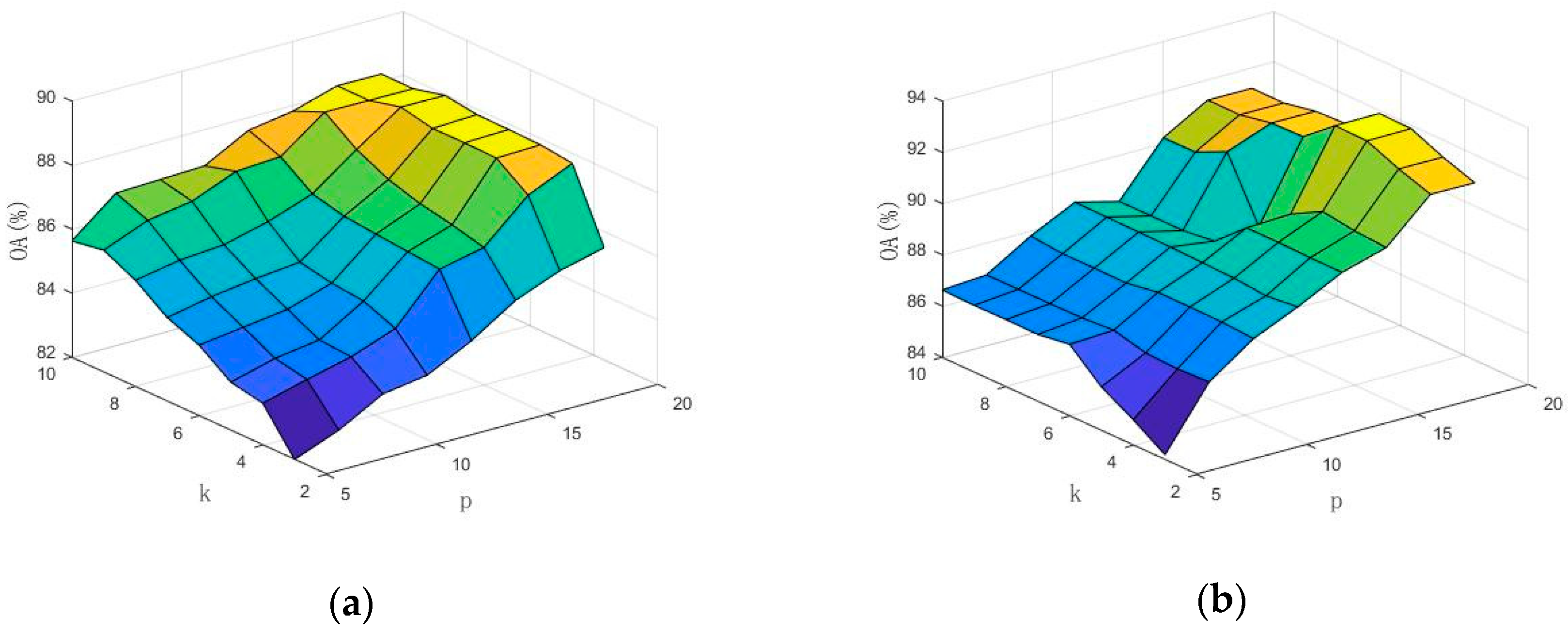
The efficient use of the spatial features of HSIs is essential to improve the classification accuracy. Therefore, in the construction of multi-manifold graphs in spatial dimensions, two parameters are extremely important: the spatial window size p and the number of near neighbors k. The spatial window size determines the degree of the spatial feature utilization of pixels. Twenty samples are selected as training samples in each category of both the IP and PU datasets, and the other samples are used as test samples. The variation ranges of parameters p and k are set as {5, 7, 9, …, 19} and {3, 4, 5, …, 10}, respectively. Figure 7 shows the classification results after dimensionality reduction obtained by setting different parameters p and k on the two datasets. In Figure 7, it can be observed that as the number of near neighbors k increases, the classification accuracy fluctuates around a fixed value on both datasets when the spatial window size p is fixed. The increase in the number of near neighbors k leads to a variable feature extraction effect on the spatial near-neighbor graph, which has an impact on the classification results. When k is fixed, the classification effect on both datasets first increases and then fluctuates around a fixed value as the spatial window size p increases. More spatial features can be captured when the spatial window size p is gradually increased. However, when the spatial window is too large, the spatial window may capture some spatial features that interfere with the dimensionality reduction effect.

4.4.3. Balancing Spectral Information Parameters α and Spatial Information Parameters β

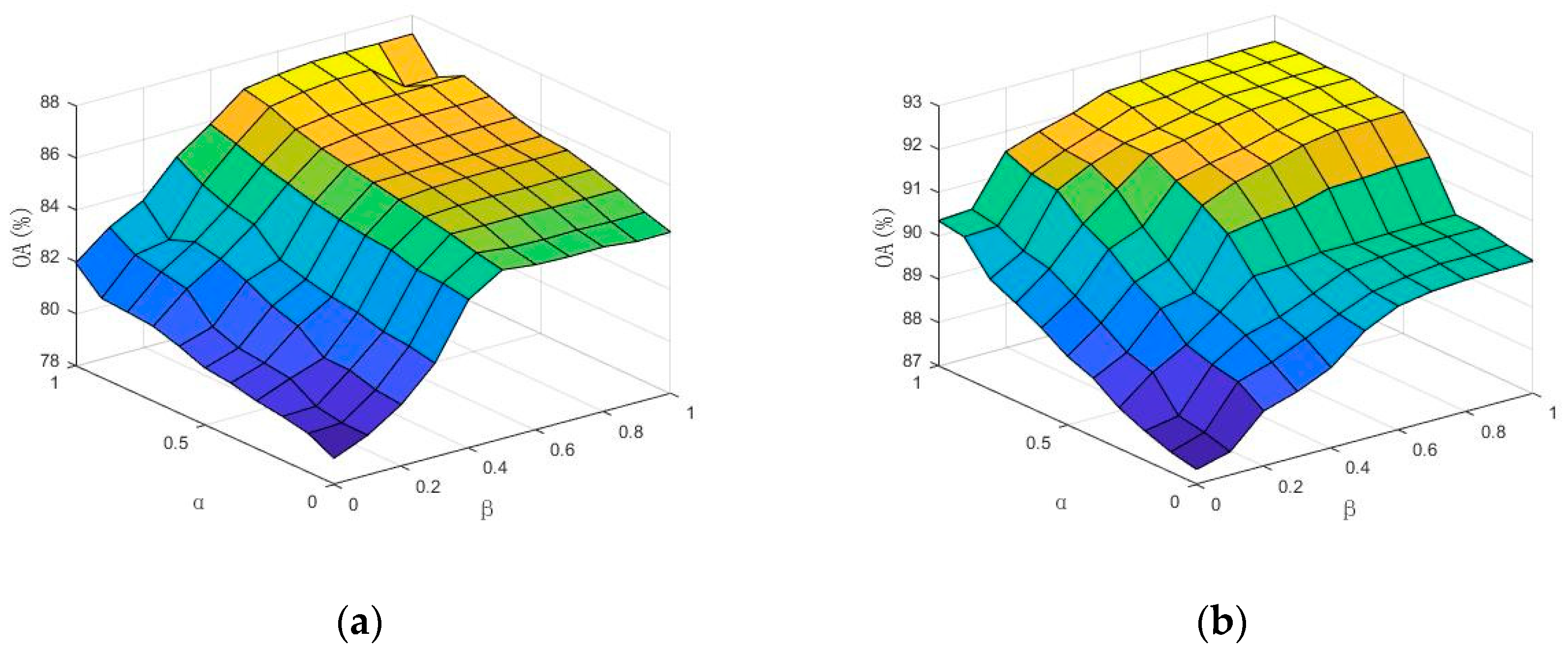
In order to evaluate the effects of balancing spectral information parameters α and spatial information parameters β on the dimensionality reduction performance, 20 samples from each category were selected as training samples on both datasets. The variation range of α and β was {0, 0.1, 0.2, …, 1}. The comparison between the dimensionality reduction effect obtained on two datasets is shown in Figure 8. In Figure 8, it can be seen that when the parameter α is a fixed value, the classification accuracy of the model gradually increases and stabilizes with the increasing parameter β. As the parameter β continues to increase, the intra-manifold maps in the spatial and spectral domains occupy an increasingly important weight in the whole near-neighbor map. In addition, when the parameter β is fixed, the classification accuracy of the model gradually increases and fluctuates about a fixed value as the parameter α increases. As a larger α indicates a stronger separation of data between inter-manifold data, it occupies an increasingly important weight in the whole near-neighbor graph. Considering the comprehensive model performance and model complexity, α = 0.6 and β = 0.7 were chosen as the two parameters used in the experiment.

4.4.4. The Dimension of the Subspace d after Dimensionality Reduction

In order to evaluate the impact of subspace dimension d on the dimensionality reduction performance, based on the a priori knowledge, the variation range of subspace dimension d is set at {5, 10, 15, …, 45}. Figure 9 shows the dimensionality reduction results obtained after selecting different subspace dimensions d on the two datasets. In Figure 9, it can be seen that among all of the algorithms, the classification accuracy of each type of algorithm increases continuously and then stabilizes as the dimension of subspace d increases. Among the algorithms, the overall classification accuracy of the algorithms in this paper is optimal. In a certain range, as the dimension of subspace d keeps increasing, the effective spatial–spectral feature information in the subspace keeps increasing, meaning that the classification accuracy of the algorithm gradually increases. However, because enough rich and discriminative features have been captured when the subspace dimension d increases to a fixed value and continues to increase, the classification accuracy of the algorithm does not continue to increase.

4.5. Ablation Experiments

To further verify the effectiveness of SAWRM and SSMMM, the classification results obtained via the experiments on the IP and PU datasets with different algorithm models (M1~M4) are shown in Table 5. M1 indicates that only the spectral multi-manifold feature extraction method is used to complete the image dimensionality reduction process. M2 indicates that both the SAWRM and spectral multi-manifold feature extraction methods are used to accomplish the image dimensionality reduction. M3 indicates that both the fixed near-neighbor pixel representation and SSMMM methods are used to accomplish image dimensionality reduction. M4 indicates that both SAWRM and SSMMM are used to accomplish the image dimensionality reduction. The number of training sets on the IP and PU datasets is 18 and 32, respectively. Other parameters are chosen as the optimal values of the parameters discussed in Section 4.4. As can be seen in Table 5, the SAWRM and SSMMM methods can improve the dimensionality reduction performance of the whole algorithm, where the simultaneous addition of both modules makes the classification accuracy of the model reach the highest value.

5. Conclusions

In view of the fact that the current single-manifold learning strategy cannot map the multi-manifold structure in hyperspectral data, we propose the model SSAMMA. Firstly, we propose a new representation based on SAWRM for HSIs. SAWRM chunks HSIs via the image segmentation algorithm and adaptively weights the samples in each super-pixel block to form a new image with more similar spectral lines for the same class of samples. Secondly, we propose a new way to construct a spatial–spectral multi-manifold map based on SSMMM. Finally, a spatial–spectral objective function is designed to adaptively obtain the optimal projection direction on each sub-manifold, which fuses the discriminative features on different sub-manifolds to improve the classification performance. We conduct an enormous number of experiments using two datasets compared to eight dimensionality reduction algorithms, demonstrating the superiority and stability of the proposed SSAMMA. The computational complexity of the algorithm may be high due to super-pixel segmentation and the construction of a multi-manifold map. Longer runtime and larger computational resources may be required when processing large-scale HSIs.

Author Contributions

Conceptualization, S.X., S.G., Q.Y. and H.G.; methodology, S.X., S.G., Q.Y. and H.G.; validation, S.G. and H.G.; formal analysis, S.G. and S.X.; investigation, S.X. and S.G.; writing—original draft preparation, S.G. and S.X.; writing—review and editing, S.G.; supervision, S.X.; project administration, S.X. and H.G.; funding acquisition, H.G. All authors have read and agreed to the published version of the manuscript.

Funding

This work was supported in part by the National Natural Science Foundation of China under Grant 62071168, the Natural Science Foundation of Jiangsu Province under Grant BK20211201, and the China Postdoctoral Science Foundation under Grant 2021M690885.

Institutional Review Board Statement

Not applicable.

Informed Consent Statement

Not applicable.

Data Availability Statement

Data are contained within in this article.

Conflicts of Interest

The authors declare no conflict of interest.

References

  1. Landgrebe, D. Hyperspectral image data analysis. IEEE Signal Process. Mag. 2002, 1, 17–28. [Google Scholar] [CrossRef]
  2. Gao, H.; Chen, Z.; Li, C. Hierarchical shrinkage multiscale network for hyperspectral image classification with hierarchical feature fusion. IEEE J. Sel. Top. Appl. Earth Observ. Remote Sens. 2021, 14, 5760–5772. [Google Scholar] [CrossRef]
  3. Gao, H.; Chen, Z.; Li, C. Shallow network based on depthwise overparameterized convolution for hyperspectral image classification. IEEE Geosci. Remote Sens. Lett. 2022, 19, 6005205. [Google Scholar] [CrossRef]
  4. Hong, D.; Gao, L.; Yao, J.; Zhang, B.; Plaza, A.; Chanussot, J. Graph convolutional networks for hyperspectral image classification. IEEE Trans. Geosci. Remote Sens. 2021, 7, 5966–5978. [Google Scholar] [CrossRef]
  5. Lv, Z.; Liu, T.; Benediktsson, J.A.; Falco, N. Land cover change detection techniques: Very-high-resolution optical images: A review. IEEE Geosci. Remote Sens. Mag. 2022, 1, 44–63. [Google Scholar] [CrossRef]
  6. Lv, Z.; Wang, F.; Cui, G.; Benediktsson, J.A.; Lei, T.; Sun, W. Spatial–spectral attention network guided with change magnitude image for land cover change detection using remote sensing images. IEEE Trans. Geosci. Remote Sens. 2022, 60, 4412712. [Google Scholar] [CrossRef]
  7. Chang, C.I. Hyperspectral anomaly detection: A dual theory of hyperspectral target detection. IEEE Trans. Geosci. Remote Sens. 2022, 60, 5511720. [Google Scholar] [CrossRef]
  8. Feng, S.; Tang, S.; Zhao, C.; Cui, Y. A hyperspectral anomaly detection method based on low-rank and sparse decomposition with density peak guided collaborative representation. IEEE Trans. Geosci. Remote Sens. 2022, 60, 5501513. [Google Scholar] [CrossRef]
  9. Zhao, C.; Li, C.; Feng, S.; Li, W. Spectral–spatial anomaly detection via collaborative representation constraint stacked autoencoders for hyperspectral images. IEEE Geosci. Remote Sens. Lett. 2022, 19, 5503105. [Google Scholar] [CrossRef]
  10. Wu, X.; Hong, D.; Chanussot, J. UIU-Net: U-Net in U-Net for infrared small object detection. IEEE Trans. Image Process. 2023, 32, 364–376. [Google Scholar] [CrossRef]
  11. Yao, J.; Hong, D.; Xu, L.; Meng, D.; Chanussot, J.; Xu, Z. Sparsityenhanced convolutional decomposition: A novel tensor-based paradigm for blind hyperspectral unmixing. IEEE Trans. Geosci. Remote Sens. 2022, 60, 5505014. [Google Scholar] [CrossRef]
  12. Chang, C.I.; Kuo, Y.M.; Chen, S.; Liang, C.C.; Ma, K.Y.; Hu, P.F. Self-Mutual Information-Based Band Selection for Hyperspectral Image Classification. IEEE Trans. Geosci. Remote Sens. 2020, 59, 5979–5997. [Google Scholar] [CrossRef]
  13. Shang, X.; Song, M.; Wang, Y.; Yu, H.; Chang, C.I. Hyperspectral target detection based on target-constrained interference-minimized band selection. In Proceedings of the IGARSS 2020–2020 IEEE International Geoscience and Remote Sensing Symposium, Waikoloa, HI, USA, 26 September–2 October 2020; pp. 2033–2036. [Google Scholar]
  14. Shaw, G.; Manolakis, D. Signal processing for hyperspectral image exploitation. IEEE Signal Process. Mag. 2002, 1, 12–16. [Google Scholar] [CrossRef]
  15. Kuo, B.C.; Landgrebe, D.A. Nonparametric weighted feature extraction for classification. IEEE Trans. Geosci. Remote Sens. 2004, 42, 1096–1105. [Google Scholar]
  16. Valle, S.; Li, W.; Qin, S.J. Selection of the number of principal components: The variance of the reconstruction error criterion with a comparison to other methods. Ind. Eng. Chem. Res. 1999, 38, 4389–4401. [Google Scholar] [CrossRef]
  17. Abbas, A.M. Image encryption based on independent component analysis and arnold’cCat map. Egypt. Inform. J. 2016, 17, 139–146. [Google Scholar] [CrossRef] [Green Version]
  18. Struc, V.; Paveic, N. Gabor-based kernel partial-least-squares discrimination features for face recognition. Informatica 2019, 20, 115–138. [Google Scholar] [CrossRef]
  19. Pang, Y.; Ji, Z.; Jiang, P. Ranking graph embedding for learning to rerank. IEEE Trans. Neural Netw. Learn. Syst. 2013, 24, 1292–1303. [Google Scholar] [CrossRef]
  20. Luo, F.; Huang, H.; Duan, Y. Local geometric structure feature for dimensionality reduction of hyperspectral imagery. Remote Sens. 2017, 9, 790. [Google Scholar] [CrossRef] [Green Version]
  21. He, X.; Deng, C.; Yan, S. Neighborhood preserving embedding. In Proceedings of the Tenth IEEE International Conference on Computer Vision, Beijing, China, 17–21 October 2005. [Google Scholar]
  22. Pu, H.; Chen, Z.; Wang, B. A novel spatial–spectral similarity measure for dimensionality reduction and classification of hyperspectral imagery. IEEE Trans. Geosci. Remote Sens. 2014, 52, 7008–7022. [Google Scholar]
  23. Deng, Y.; Li, H.; Pan, L. Modified tensor locality preserving projection for dimensionality reduction of hyperspectral images. IEEE Geosci. Remote Sens. Lett. 2018, 15, 77–281. [Google Scholar] [CrossRef]
  24. Cheng, B.; Yang, J.; Yan, S. Learning with l1-graph for image analysis. IEEE Trans. Image Process. 2010, 19, 58–66. [Google Scholar] [CrossRef] [PubMed]
  25. Wang, L.Z.; Huang, H.; Feng, H.L. Application of Multilinear Local and Global Preserving Embedding in Hyperspectral Remote Sensing Image Classification. J. Comput.-Aided Des. Comput. Graph. 2012, 24, 780–786. [Google Scholar]
  26. Huang, H.; Li, Z.; Pan, Y. Multi-feature manifold discriminant analysis for hyperspectral image classification. Remote Sens. 2019, 11, 651. [Google Scholar] [CrossRef] [Green Version]
  27. Li, J.; Zhang, H.; Zhang, L. Joint collaborative representation with multitask learning for hyperspectral image classification. IEEE Trans. Geosci. Remote Sens. 2014, 52, 5923–5936. [Google Scholar] [CrossRef]
  28. Kang, X.; Li, S.; Benediktsson, J.A. Spectral-spatial hyperspectral image classification with edge-preserving filtering. IEEE Trans. Geosci. Remote Sens. 2014, 52, 2666–2677. [Google Scholar] [CrossRef]
  29. Zhang, S.; Li, S.; Fu, W. Multiscale superpixel-based sparse representation for hyperspectral image classification. Remote Sens. 2017, 9, 139. [Google Scholar] [CrossRef] [Green Version]
  30. Liu, H.; Li, W.; Xia, X. Superpixelwise collaborative-representation graph embedding for unsupervised dimension reduction in hyperspectral imagery. IEEE J. Sel. Top. Appl. Earth Obs. Remote Sens. 2021, 14, 4684–4698. [Google Scholar] [CrossRef]
  31. Dong, Y.; Jin, Y.; Cheng, S. Clustered multiple manifold metric learning for hyperspectral image dimensionality reduction and classification. IEEE Trans. Geosci. Remote Sens. 2022, 60, 5516813. [Google Scholar] [CrossRef]
  32. Achanta, R.; Shaji, A.; Smith, K.; Lucchi, A.; Fua, P.; Süsstrunk, S. SLIC superpixels compared to state-of-the-art superpixel methods. IEEE Trans. Pattern Anal. Mach. Intell. 2012, 34, 2274–2281. [Google Scholar] [CrossRef] [Green Version]
  33. Wu, D.Y.; Ma, L. Multi-manifold LE algorithm for dimension reduction and classification of multitemporal hyperspectral image. Remote Sens. Land Resour. 2018, 30, 80–86. [Google Scholar]
  34. Li, D.Q. Spatial-Spectral Graph Embedding for Dimensionality Reduction of Hyperspectral Data. Ph.D. Thesis, China University of Mining and Technology, Beijing, China, 2019. [Google Scholar]
  35. Lu, J.; Tan, Y.P.; Wang, G. Discriminative multi-manifold analysis for face recognition from a single training sample per person. IEEE Trans. Pattern Anal. Mach. Intell. 2012, 35, 39–51. [Google Scholar] [CrossRef] [PubMed]
  36. Wong, W.K. Discover latent discriminant information for dimensionality reduction: Non-negative sparseness preserving embedding. Pattern Recognit. 2012, 45, 511–1523. [Google Scholar] [CrossRef]
  37. Liu, B.; Zhou, Y.; Xia, Z.G. Spectral regression based marginal fisher analysis dimensionality reduction algorithm. Neurocomputing 2018, 277, 101–107. [Google Scholar] [CrossRef]
  38. Wu, D.Y.; Ma, L. Application of Multi-manifold LE Algorithm in Dimensionality Reduction and Classification of Hyperspectral Images. Remote Sens. Land Resour. 2018, 30, 7. [Google Scholar]
  39. Jiang, J.; Ma, J.; Chen, C.; Wang, Z.; Cai, Z.; Wang, L. Superpca: A superpixelwise pca approach for unsupervised feature extraction of hyperspectral imagery. IEEE Trans. Geosci. Remote Sens. 2018, 56, 4581–4593. [Google Scholar] [CrossRef] [Green Version]
  40. Huang, H.; Shi, G.; He, H. Dimensionality reduction of hyperspectral imagery based on spatial–spectral manifold learning. IEEE Trans. Cybern. 2020, 50, 2604–2616. [Google Scholar] [CrossRef] [Green Version]
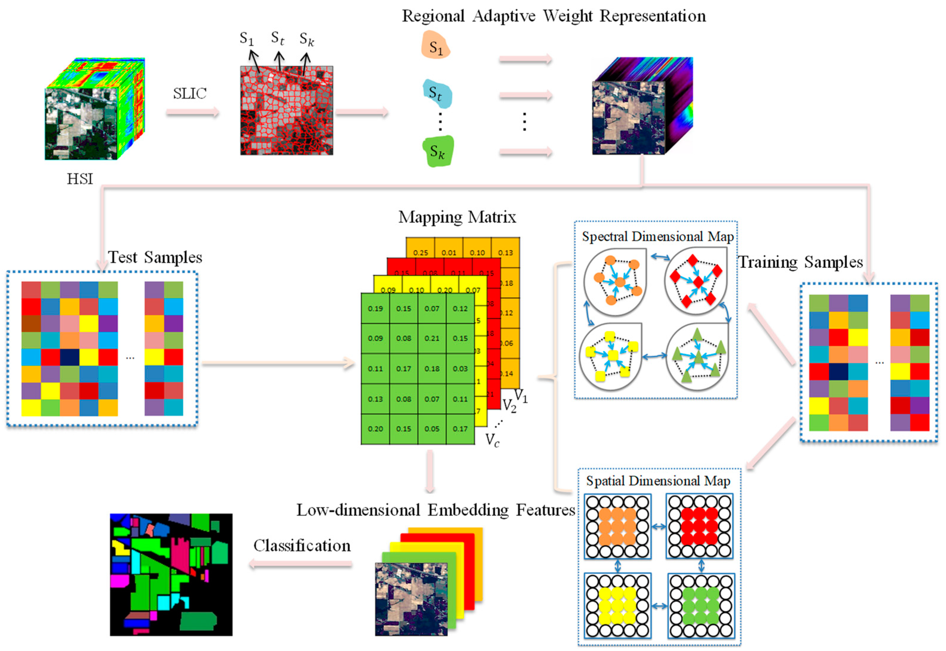
Figure 1. The overall framework of the proposed SSAMMA.
Applsci 13 09180 g001
Figure 2. IP dataset: (a) false-color composite image; (b) ground-truth map.
Applsci 13 09180 g002
Figure 3. UP dataset: (a) false-color composite image; (b) ground-truth map.
Applsci 13 09180 g003
Figure 4. Classification results of different dimensionality reduction algorithms using IP dataset: (a) GT; (b) PCA; (c) LPP; (d) MFA; (e) NSPE; (f) MLE; (g) MMDA; (h) SSMRPE; (i) SPCA; (j) SSAMMA.
Applsci 13 09180 g004
Figure 5. Classification results of different dimensionality reduction algorithms using UP dataset: (a) GT; (b) PCA; (c) LPP; (d) MFA; (e) NSPE; (f) MLE; (g) MMDA; (h) SSMRPE; (i) SPCA; (j) SSAMMA.
Applsci 13 09180 g005
Figure 6. Classification results of different parameters a and b using two data sets: (a) IP dataset; (b) PU dataset.
Applsci 13 09180 g006
Figure 7. Classification accuracy under different values of spatial window size p and the number of near neighbors k: (a) IP dataset; (b) PU dataset.
Applsci 13 09180 g007
Figure 8. Effect of parameters α and β using dimensionality reduction results: (a) IP dataset; (b) PU dataset.
Applsci 13 09180 g008
Figure 9. Effect of dimensionality d using two data sets: (a) IP dataset; (b) PU dataset.
Applsci 13 09180 g009
Table 1. Ground object category for the IP dataset.
Category NumberCategory NameSample NumberColor
1Alfalfa46Applsci 13 09180 i001
2Corn-notill1428Applsci 13 09180 i002
3Corn-mintill830Applsci 13 09180 i003
4Corn237Applsci 13 09180 i004
5Grass-pasture483Applsci 13 09180 i005
6Grass-trees730Applsci 13 09180 i006
7Grass-pasture-mowed28Applsci 13 09180 i007
8Hay-windrowed478Applsci 13 09180 i008
9Oats20Applsci 13 09180 i009
10Soybean-notill972Applsci 13 09180 i010
11Soybean-mintill2455Applsci 13 09180 i011
12Soybean-clean593Applsci 13 09180 i012
13Wheat205Applsci 13 09180 i013
14Woods1265Applsci 13 09180 i014
15Buildings-grass-trees-drives386Applsci 13 09180 i015
16Stone-steel-towers93Applsci 13 09180 i016
Total 10,249
Table 2. Ground object category for the UP dataset.
Category NumberCategory NameSample NumberColor
1Asphalt6631Applsci 13 09180 i017
2Meadows18,649Applsci 13 09180 i018
3Gravel2099Applsci 13 09180 i019
4Trees3064Applsci 13 09180 i020
5Painted metal sheets1345Applsci 13 09180 i021
6Bare Soil5029Applsci 13 09180 i022
7Bitumen1330Applsci 13 09180 i023
8Self-blocking bricks3682Applsci 13 09180 i024
9Shadows947Applsci 13 09180 i025
Total 42,776
Table 3. Classification accuracy (%) of various algorithms using IP dataset.
No.PCALPPMFANSPEMLEMMDASSMRPESPCASSAMMA
C173.6784.9786.3872.0768.8585.0881.2398.8796.23
C292.5679.9689.2966.8572.0680.7480.5890.5490.87
C382.0558.9985.6063.2070.6765.0374.0991.2793.96
C460.3932.0258.9267.2848.8268.2571.2093.8292.38
C595.4394.0795.4772.8179.5893.2893.2897.2896.97
C697.2297.2397.5676.5889.2598.5397.5697.0199.78
C780.1145.0684.6866.5068.9184.3191.6591.5295.86
C896.5897.8998.7879.2193.6398.6097.2898.0799.69
C985.7068.0087.8266.0057.9868.8769.8798.6494.22
C1073.3562.2575.6567.2568.4673.3878.9976.4978.87
C1185.6885.6284.8788.1675.7283.6485.3190.7292.34
C1268.9771.0668.3671.0262.3981.2575.8285.2589.70
C1395.0299.3095.1380.0388.2499.0198.8699.52100
C1493.6597.6194.6595.1683.1897.1297.5897.3498.53
C1565.2262.3568.3057.5550.0372.4597.3690.6588.38
C1695.8386.5196.5676.8571.3488.2468.4591.3692.66
OA82.6583.0286.2572.3578.2385.8688.7591.3491.59
AA80.2867.3383.0670.4775.6283.0686.3792.6092.76
K81.2676.8784.8771.5676.4484.5787.6090.6790.48
T(s)0.174.267.938.5720.1530.5442.820.4846.52
Table 4. Classification accuracy (%) of various algorithms using UP dataset.
No.PCALPPMFANSPEMLEMMDASSMRPESPCASSAMMA
C183.2085.8687.3885.9682.0992.4592.6479.6495.61
C290.0591.5095.2691.6389.4794.6597.8993.0897.85
C363.6864.2275.0356.0660.5668.7376.2197.5492.03
C478.1481.0382.1779.9072.3890.7681.2385.3388.38
C597.3897.4898.2592.7495.6588.2399.5896.8899.85
C686.5662.4767.2859.4279.2679.1595.6694.8097.21
C781.8783.8888.2465.5075.6073.2487.4592.3898.43
C875.1278.8678.8167.2471.8385.4381.1892.5589.07
C998.5098.5198.5269.8894.5795.3299.7695.5399.38
OA85.9386.0487.3874.2679.8287.5892.3590.9696.53
AA82.6585.3586.5070.4576.6786.8391.1991.9794.12
K82.7682.7683.5772.1273.7886.7291.3288.1695.38
T(s)0.6896.229.64106.5424.6241.2844.640.5110.71
Table 5. Classification accuracy of different models using IP and PU datasets.
DatasetModelModuleMetrics
SAWRMSSMMMOAAAK
IPM1××82.6580.7279.68
M2 ×88.0487.1386.19
M3× 88.2787.3686.50
M4 90.5689.7188.02
PUM1××92.8791.4890.16
M2 ×95.1194.0093.14
M3× 95.3494.2994.05
M4 97.8697.0696.22
Disclaimer/Publisher’s Note: The statements, opinions and data contained in all publications are solely those of the individual author(s) and contributor(s) and not of MDPI and/or the editor(s). MDPI and/or the editor(s) disclaim responsibility for any injury to people or property resulting from any ideas, methods, instructions or products referred to in the content.