Dim Staring Debris Targets Detection Method with Dense Long Trailing Star

Featured Application

The method studied in this paper is applied to the debris detection on-board, especially the dim targets and the occluded by a long trailing star.

Abstract

With the gradual increase in spacecraft in orbit, space debris monitoring has become the key to the sustainable development of space missions. A staring debris detection method is proposed for high-density stars with long tails. In order to solve the problem that the gray level of a long trailing image is not stable and continuous, rectangular fitting is used to complete the aggregation of the trailing image and reduce the influence of noise on the trailing information. The occluded state of the target was analyzed, the feature calculation method was improved, the semi-occluded scene was statistically classified, the fully connected network (FCN) based finite point feature was accurately classified, and the semi-occluded image was extracted. Based on the extracted semi-occluded image, the inter-frame association can improve the success probability of target association and realize the effective detection and tracking of debris. The detection accuracy was tested for the changing inter-frame interval and signal-to-noise ratio (SNR), and the relationship between the index parameters and key parameters was given. Compared with previous literature, this design can detect and track the occluded target with a detection rate of more than 90% and a false alarm rate of less than 10%.

1. Introduction

With the continuous development of civil spaceflight and the intensive launch of satellite missions, space debris has become an important factor affecting the safe and reliable execution of current aerospace missions [1]. In the early stage, debris monitoring mainly relied on ground-based radar and astronomical telescopes. However, with the increasing number of debris, limited by observation time and field of view, research on space-based debris monitoring has been gradually turned to in the past decade [2].

Space-based debris monitoring mainly relies on optical cameras to image the debris target, obtain astronomical data similar to a “star list”, and confirm the target information according to the difference in the motion state between the star background and the target [3]. However, with the increase in fragment targets to small scales such as decimeter level and centimeter level, the number of targets in the image and the complexity of content gradually bring great difficulty to the process of information extraction [4]. For remote and small-scale weak targets, the target-follow camera long exposure mode is often used to achieve the target-background SNR, which is sufficient for detection and recognition [5]. In this mode, the staring target forms a point target on the image, the background star forms a long trailing shape, and the non-gazing target forms shapes with different trailing lengths [6].

In the early stage, space debris target detection mainly relied on long-term observation for orbit determination to judge the target [7]. With the development of image processing technology, there are two main types of image processing-based methods: One is to obtain the mapping relationship between a single image and the celestial sphere according to the match of the camera imaging data and the star list, and then perform matching and eliminating for each star target to finally retain the fragment target information [8]. The other is to conduct registration and difference comparison judgment for the front and back frames of continuous imaging and distinguish target information based on different time domain distributions of stars and debris targets [9]. These two methods have good accuracy in data processing under the background of short trailing stars [10], and can give consideration to both real-time performance and accuracy under high SNR by relying on inter-frame differential calculation [11].

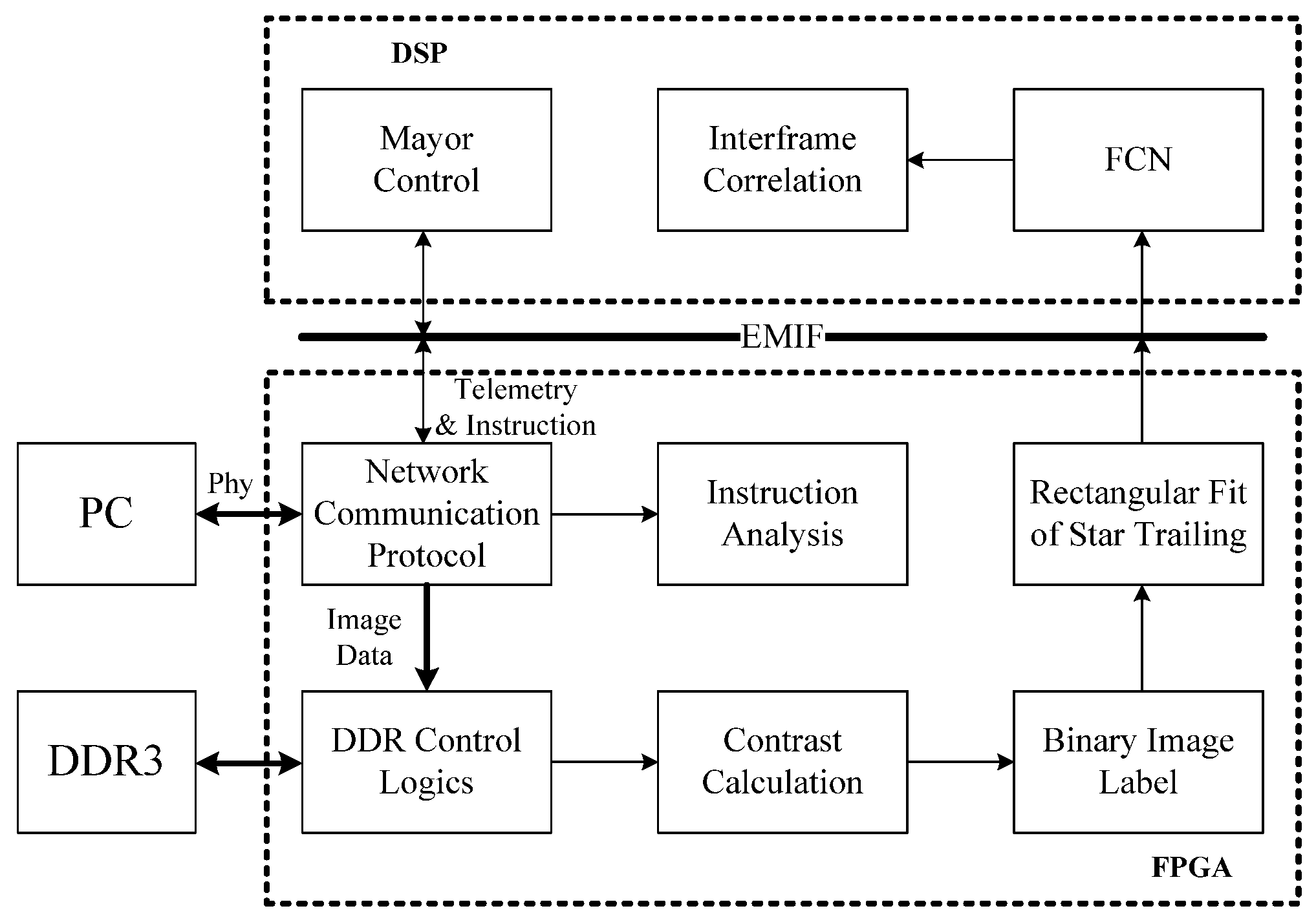
The early algorithm mainly aimed at the point target, combined with multi-frame accumulation, to achieve the multi-frame information of the moving target to form a shape similar to “dotted line”, and the line detection method was used to calculate the position and trajectory [12]. The detection of orbiting debris targets mainly relies on DSP and FPGA to form a heterogeneous computing platform to achieve real-time image processing [13]. There are also some methods to achieve trajectory by high-precision positioning of the target [14]. In the case that multiple debris targets exist simultaneously in the same field of view, the method based on a traditional tracking algorithm can also be adopted [15]. The recent method partially takes deep learning into consideration and uses a deep convolutional network to realize saliency detection for small fragment targets [16]. In literature [17], a fast grid neural network was used to complete the recognition of debris targets, which greatly improved the calculation speed while ensuring recognition accuracy. According to literature [18], the target has a significantly shorter tail compared with the stellar background, and the network-based detection can be realized through the training and learning of target data. The effective processing of weak targets is still the focus of debris monitoring at present. The method based on topological scanning proposed in literature [19] can detect and process a small number of trailing scenes. Once the trailing tail is too long, the target and star are likely to be superposed, which will lead to the failure of inter-frame correlation of target information.

To sum up, it can be seen that the monitoring of orbiting debris targets is mainly based on the motion difference between the target and the stellar background, and the information extraction of the debris target is completed by feature detection, association tracking, and other methods according to the predicted state parameters [20,21]. The scene solved by the previous algorithm is relatively simple, mainly facing the “sparse” background and target scene. In practical application, especially for some specific extremely weak targets, the background star will form a long tail, which will affect the target detection.

In this paper, we propose a method for detecting faint staring debris in the background of dense stars with long trailing tails. The gray level of the long trailing image is not stable and continuous, and the long tail may occlude the possible debris target. In these scenarios, the faint debris target can hardly be detected. We conduct the rectangle contour fitting to the stellar tails, as the angle and length of the trailing star can be predicted. Then we obtain the image with the stellar tail, and the debris target superposed together, which can be analyzed in three cases. These images are put into the fully connected network (FCN), which can tell which case the images belong to, then we can obtain the information of the occluded faint debris target. Aiming at the problem that the inter-frame association cannot be sustained due to the occlusion point target of star trailing, the inter-frame association is carried out based on the extracted semi-occluded image to improve the success probability of target association and realize the effective detection and tracking of debris.

The structure of this paper is as follows: Section 2 presents the problem and the corresponding solution algorithm; Section 3 gives the engineering implementation framework. Section 4 presents the experimental results and the comparison with previous algorithms. Section 5 concludes the paper.

2. Semi-Occluded Object Detection Algorithm Based on FCN

The staring debris mode in the background of long trailing stars aims to solve two problems in the process of target observation: one is that the debris target is too weak and has to rely on long time exposure to improve its SNR; the other is to reduce the SNR of the fixed stars by the long trailing tail of the background star to prevent the high density of the background fixed star from affecting the detection of the debris target. However, this mode also brings two new problems: one is that the long tail of the star leads to the occlusion of the debris target by the tail, which makes the conventional 3~5 frame association method ineffective; the other is that the tail is too long, causing the tail itself to be split into multiple segments, forming more false alarms.

By focusing on these problems, this section presents an object detection method based on a single-frame image, which integrates traditional multi-frame association to realize object tracking. It mainly includes four parts: simulation scene and parameter description, trailing aggregation based on rectangle fitting, semi-occluded target clustering recognition based on FCN, and multi-frame association tracking.

2.1. Simulation Scenario and Parameter Description

The simulation parameters are shown in

Table 1. Description of simulation parameters.

No.	Symbol	Parameter	Value
1	Lf	Start trailing length	26 pixels
2	Wf	Start trailing width	4 pixels
3	Ld	Debris size	3 × 3 pixels
4	Fi	Inter-frame spacing	50 pixels
5	SNR	Signal-to-noise ratio	5
6	J	Debris inter-frame jitter	0.5 pixel
7	Pi	Mean stellar spacing	20 pixels
8	$\theta$	Trailing angle	70 degrees

. The stellar trailing imaging length is 26 pixels, and the width is 3–4 pixels. The imaging size of the debris target is 3 × 3 pixels; the inter-frame imaging interval is 32 pixels; the SNR of both star and target is five; the position difference of debris between frames is 0.5 pixels. The average distance between stars is 20 pixels.

Only weak targets are considered, and the generation of bright and large debris targets and stars is not considered, nor are the effects of bright and large targets on the imaging of weak targets considered.

A total of 100 groups of continuous image data were generated, with 15 consecutive frames in each group. Considering the effectiveness of simulation and testing, only gaze imaging is considered for the debris point target, and the debris target with other motion conditions is not considered in this paper.

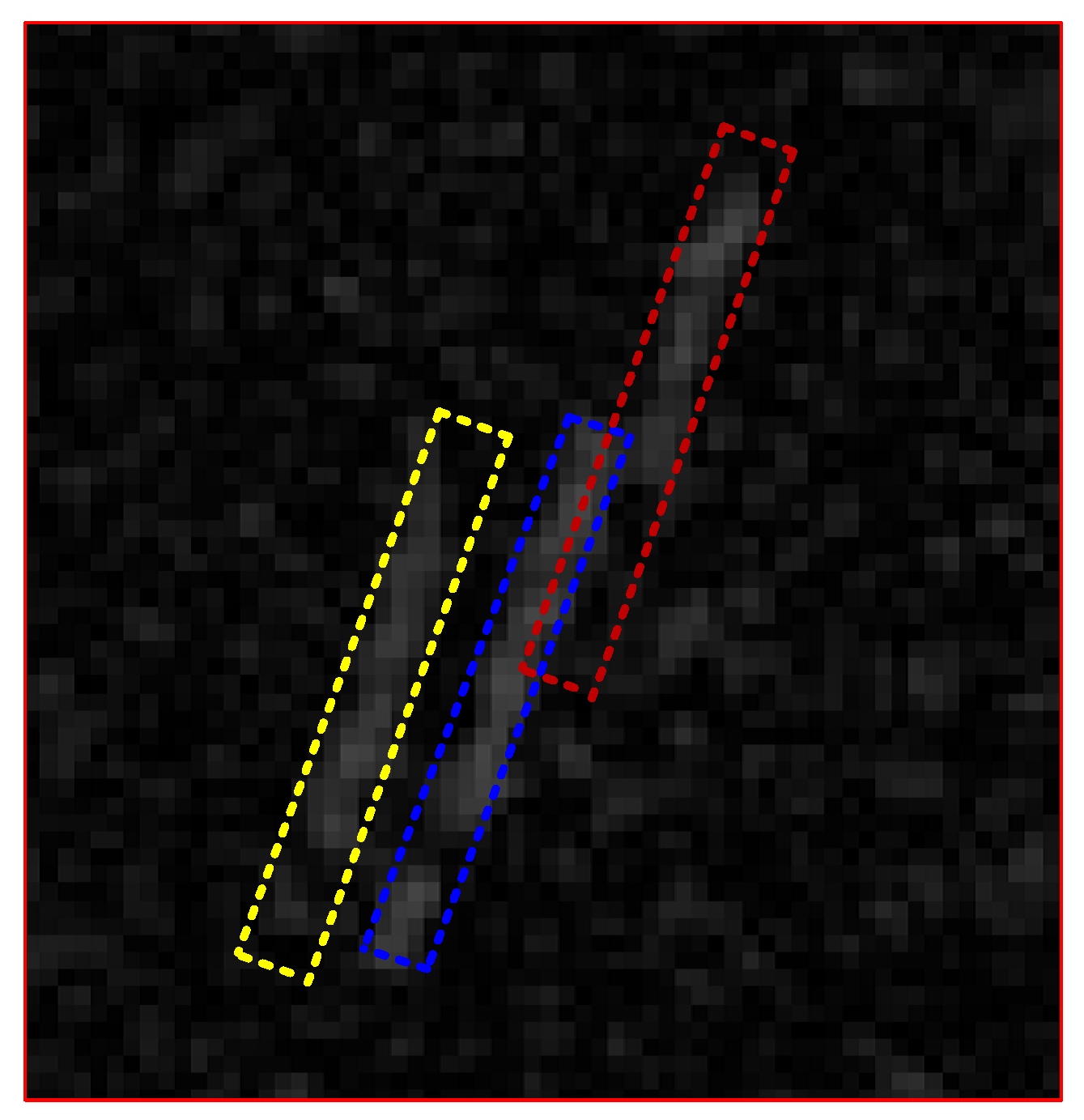
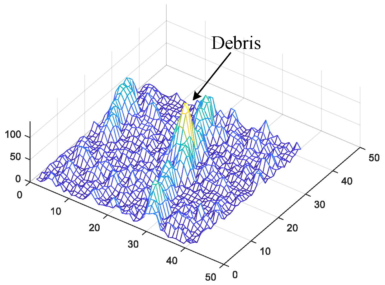
Figure 1 shows the superposition data of three frames of images. Red, green, and blue, respectively, represent the trailing stars of the three frames before and after, and the debris point target is in the center of the image. Figure 2 shows the gray levels of the local target and the star. It can be seen that the amplitude of the star trailing is discontinuous and fluctuates greatly under the influence of noise, and the middle of the trailing is prone to “fracture”. Therefore, the process should not only eliminate the background through the motion difference between the frames, but also identify the whole trailing information according to the distribution features of the image.

2.2. Trailing Aggregation Based on Rectangular Fitting

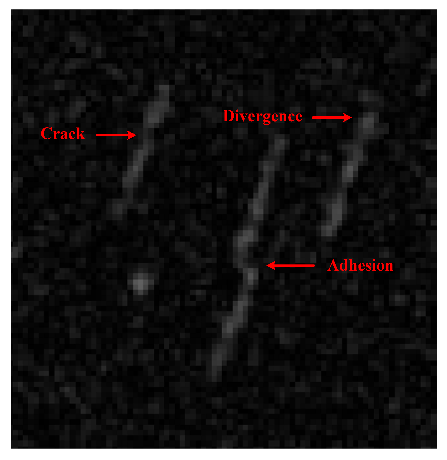
Due to noise interference and low SNR condition, stellar tails often appear in an “unstable” state in images. These states will seriously interfere with the image processing, mainly including three cases (as shown in Figure 3): The middle part of the trailing tail is broken, “Crack”; The end of the trailing tail is attached to other trailing tails, “Adhesion”; The trailing end diverges and becomes difficult to determine the edge, “Divergence”. Traditional image processing methods can hardly solve these three problems.

In order to ensure the accuracy of subsequent detection, the influence of the above problems must be eliminated first. Considering that both the angle and length of the trailing star can be predicted, the simplified rectangular fitting method is adopted here to conduct a contour search for the trailing target and finally form the edge rectangle box with the minimum error.

The main rectangle contour fitting algorithm includes the following four steps:

Step 1 (contrast segmentation calculation): Denote $I_N$ as the image, where N is the size. Use the 3 × 3 and 7 × 7 square operator, and denote $I_d$ as the contrast of $I_N$, where $T_d$ is the threshold. $x,y\in [0,N-1]$ and $x,y\in Z^{+}$, the formula for calculating the contrast is as follows:

$$I_d(x,y)=\left\{\begin{array}{c}1,\frac{{\displaystyle \sum _{i=-1}^1{\displaystyle \sum _{j=-1}^1{I}_N(x+i,y+j)}}}{{\displaystyle \sum _{i=-3}^3{\displaystyle \sum _{j=-3}^3{I}_N(x+i,y+j)}-{\displaystyle \sum _{i=-1}^1{\displaystyle \sum _{j=-1}^1{I}_N(x+i,y+j)}}}}\ge T_d.\\ 0,else.\end{array}\right.$$

(1)

Step 2 (binary labeling): Traditional binary annotation calculation is performed on $I_d$ to obtain M target sets:

$$I_b(m)=[(x_{(0,m)},y_{(0,m)}),(x_{(1,m)},y_{(1,m)}),\cdots ,(x_{(K_m-1,m)},y_{(K_m-1,m)})]$$

(2)

where, m is denoted as the m-th target, and $m\in [0,M-1]$, $m\in Z^{+}$; $K_m$ is the valid pixel number of the labeled target; $(x_{(k_m,m)},y_{(k_m,m)})$ represents the coordinates of the $k_m$ pixel of the m-th labeled target, and $k_m\in [0,K_m-1]$, $k_m\in Z^{+}$.

Step 3 (trailing rectangle generation): For any marked target $I_b(m)$, the position coordinates of its centroid $I_c(m)$ are obtained as follows:

$$I_c(m)=[\frac{{\displaystyle \sum _{k_m=0}^{K_m-1}{x}_{(k_m,m)}}}{K_m},\frac{{\displaystyle \sum _{k_m=0}^{K_m-1}{y}_{(k_m,m)}}}{K_m}]$$

(3)

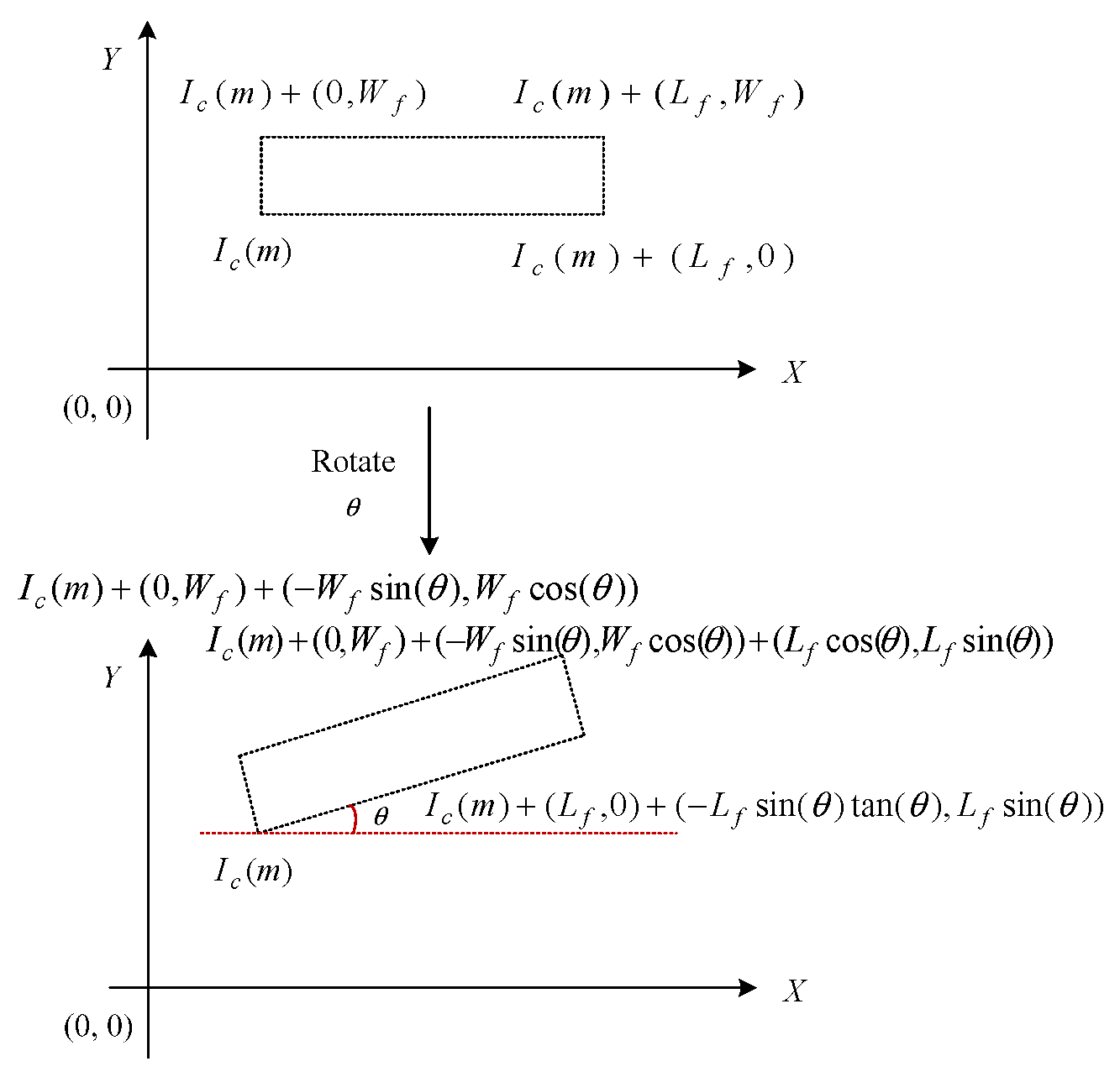
The reason why gray value weighting is not used in Equation (3) is that the target width is only three to four pixels, which is greatly disturbed by noise, and the weighting will cause more calculation errors. The center of mass of the m-th marked target is taken as any point in the rectangle, and the trailing angle $\pm \theta$ of the star is taken as the search direction to conduct the fitting rectangular box search.

The fitting process is shown in Figure 4. W_f = 4, L_f = 26. The number of rectangles is, at most, 4W_f L_f = 416. The cyan dot is the centroid of the binary-labeled region. When the rotation angle is $\theta$, the rectangle with $I_c(m)$ as the lower left point is shown in Figure 5. Through any point in the rectangle, the coordinate of the lower left corner of the matrix can be calculated, and then the coordinate of the four corners of the rectangle can be obtained so as to obtain the generating rectangle set $R(m)$ of the m-th labeled target. $R(m,q)$ denotes the set of rectangles with width and length W_f and Lf at any point with $I_c(m)$, and q denotes the q-th rectangle.

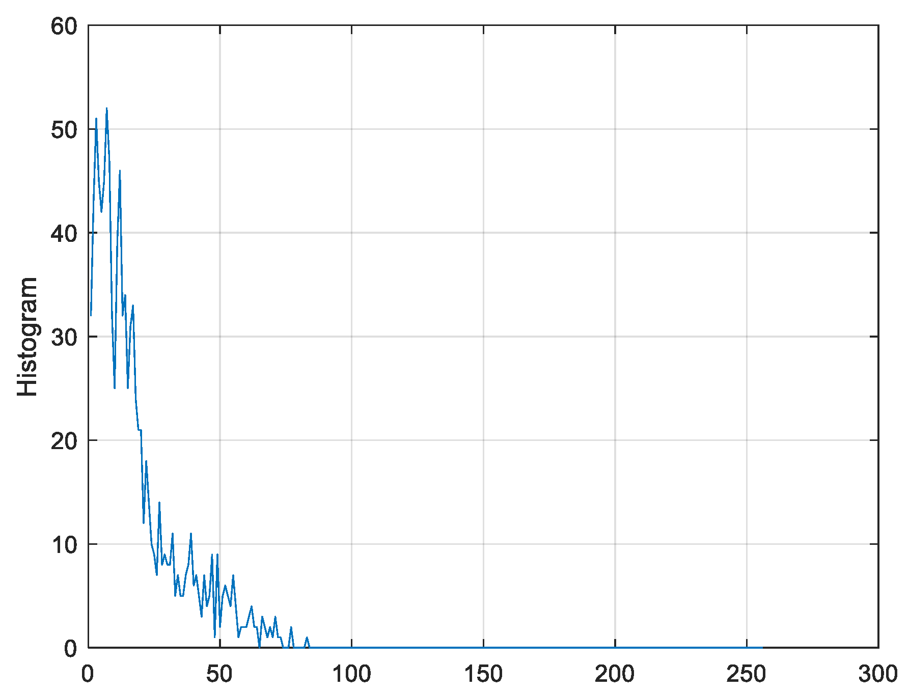
Step 4 (trailing rectangle fitting): The corresponding image region $I_N(R(m,q))$ is deduced according to $R(m,q)$, and then the gray summation $S(m,q)$ and histogram $h(m,q)$ in the rectangular region are calculated. Therefore, the optimal rectangle solution constraint is shown in Equation (4).

$$\left\{\begin{array}{c}{S}_{\min }\le S(m,q)\le S_{\max }\\ \min ({\displaystyle \sum |h(m,q)-h_{st}{|}^2})\end{array}\right.$$

(4)

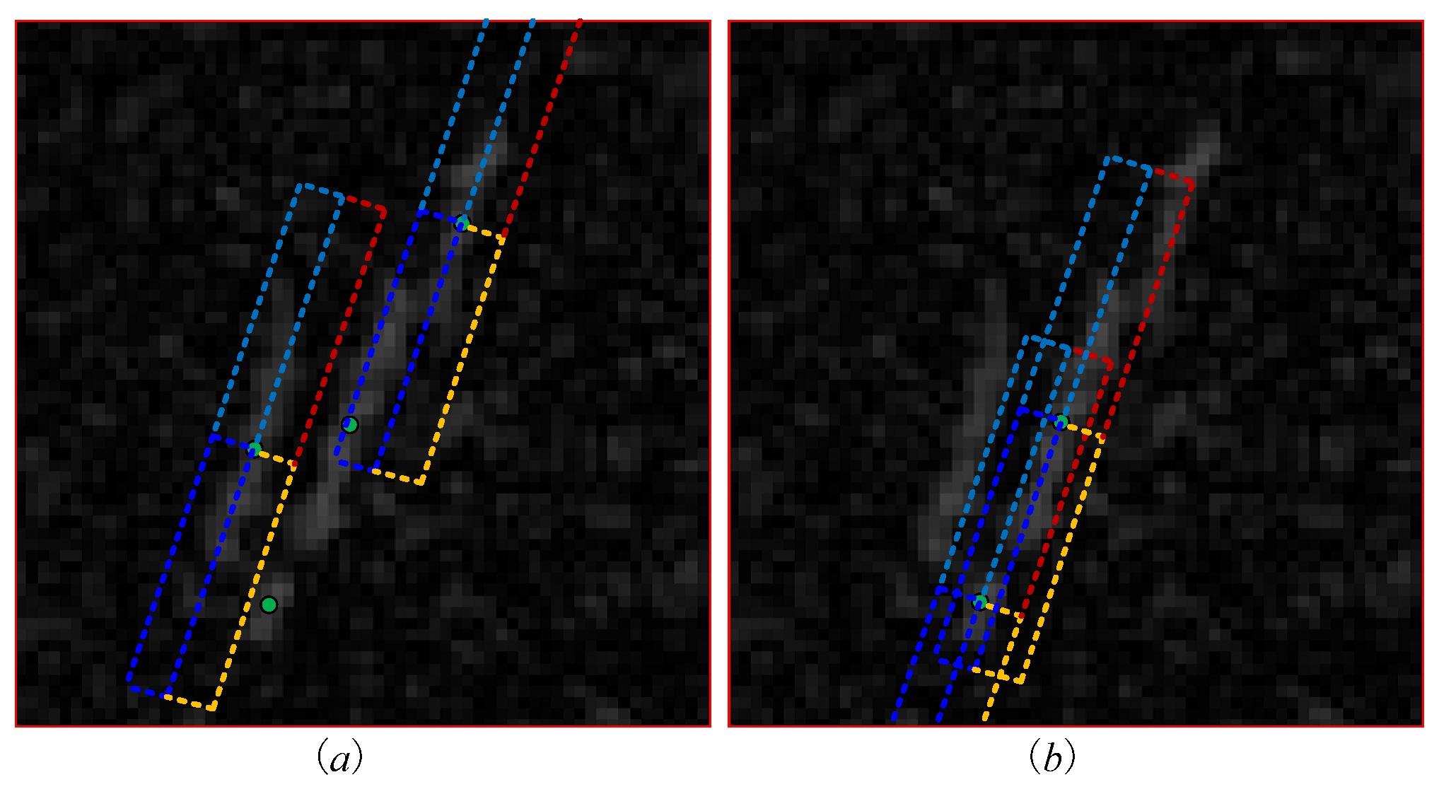
Among them, $S_{\min }$ and $S_{\max }$ are the upper and lower limits of gray summation in the rectangular area and $h_{st}$ is the histogram of trailing targets in the standard rectangular area. The three thresholds are obtained statistically and used to obtain the optimal rectangular fitting by constraint Equation (4). Figure 6 shows the histogram features of the rectangular region of the trailing image. Figure 7 shows the results of the optimal rectangle fitting.

2.3. Semi-Occluded Target Clustering Recognition Based on Edge Features

After the tail aggregation calculation, the interference of noise on the stellar tail and among the stellar tail regions is eliminated. However, in the process of detecting the debris target, they will still be blocked by the star’s trailing tail. This section will analyze several possible situations, mainly explain the features of the debris target under the occlusion in detail, and give the solution.

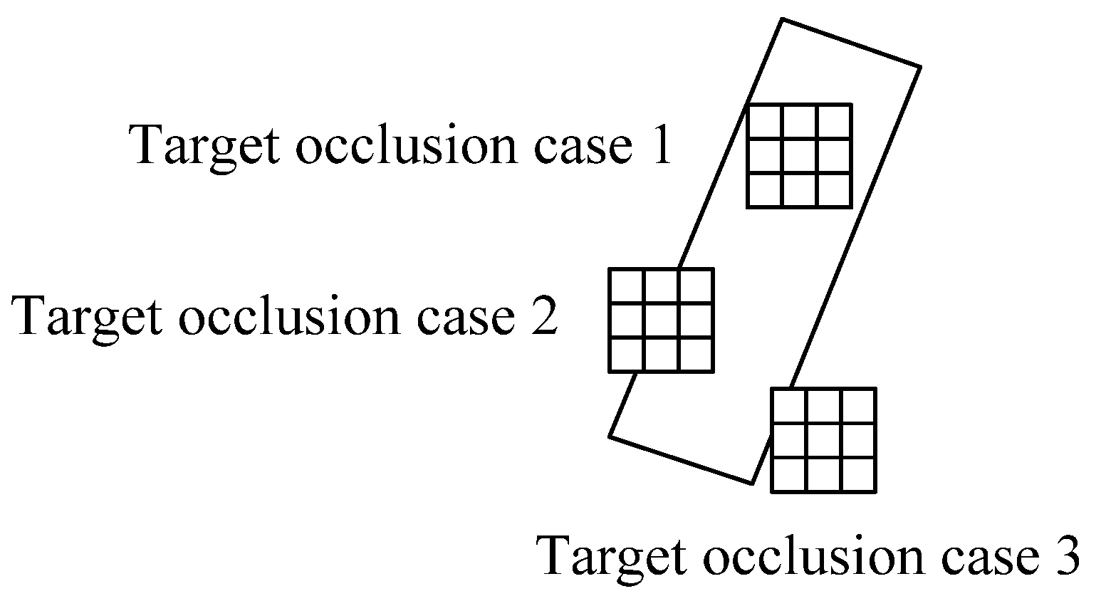
Considering the star trailing width W_f = 4 and the fragment target size L_d = 3, when occlusion occurs, it can be divided into three types according to the occlusion size as in Figure 8.

Case one: Occlusion is more than 2/3, which means that only one line of the debris target exposes the star trail. In this case, the debris target and the star trail are superimposed. Although there is local brightness accumulation, it is difficult to distinguish due to the noise;

Case two: When the occlusion is between 2/3 and 1/5, there are more than two lines of star trailing. In this case, an obvious bump is formed at the edge of the trailing star, and the bump has light and dark changes, which is obviously different from the noise bump. A large number of sample extraction statistical features need to be formed by the fragment target extraction;

Case three: When the occlusion is below 1/5, the debris target has only local contact with the stellar tail, and such occlusion is easier to distinguish on the basis of the rectangular fitting.

The distribution of occluded targets is shown in Figure 9 as a Gaussian distribution, while the star trailing statistics are mainly Rayleigh distribution. Therefore, in cases two and three, debris targets can be distinguished according to different distributions.

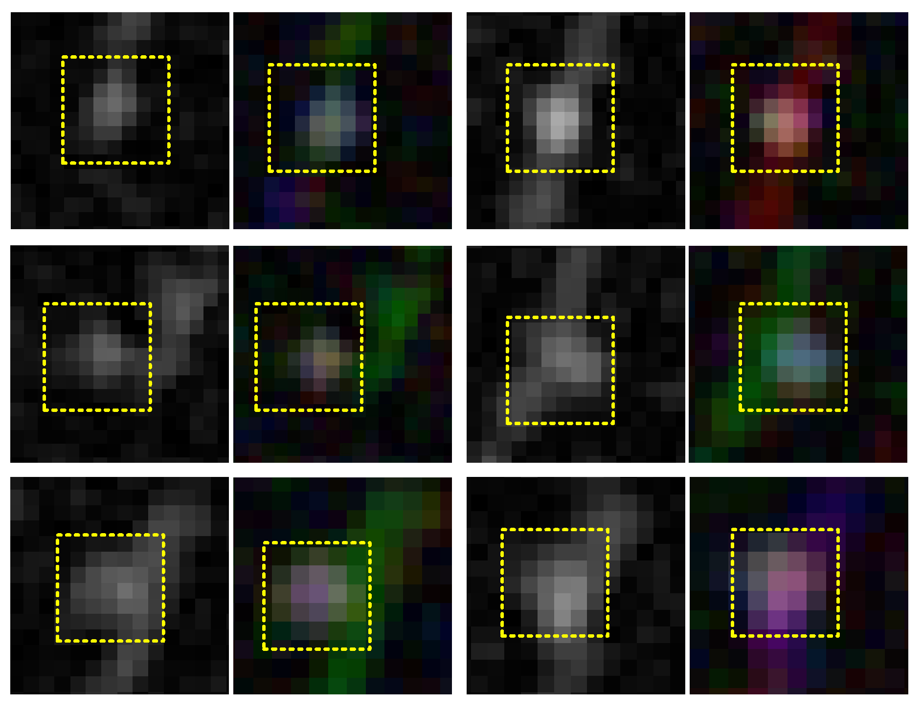
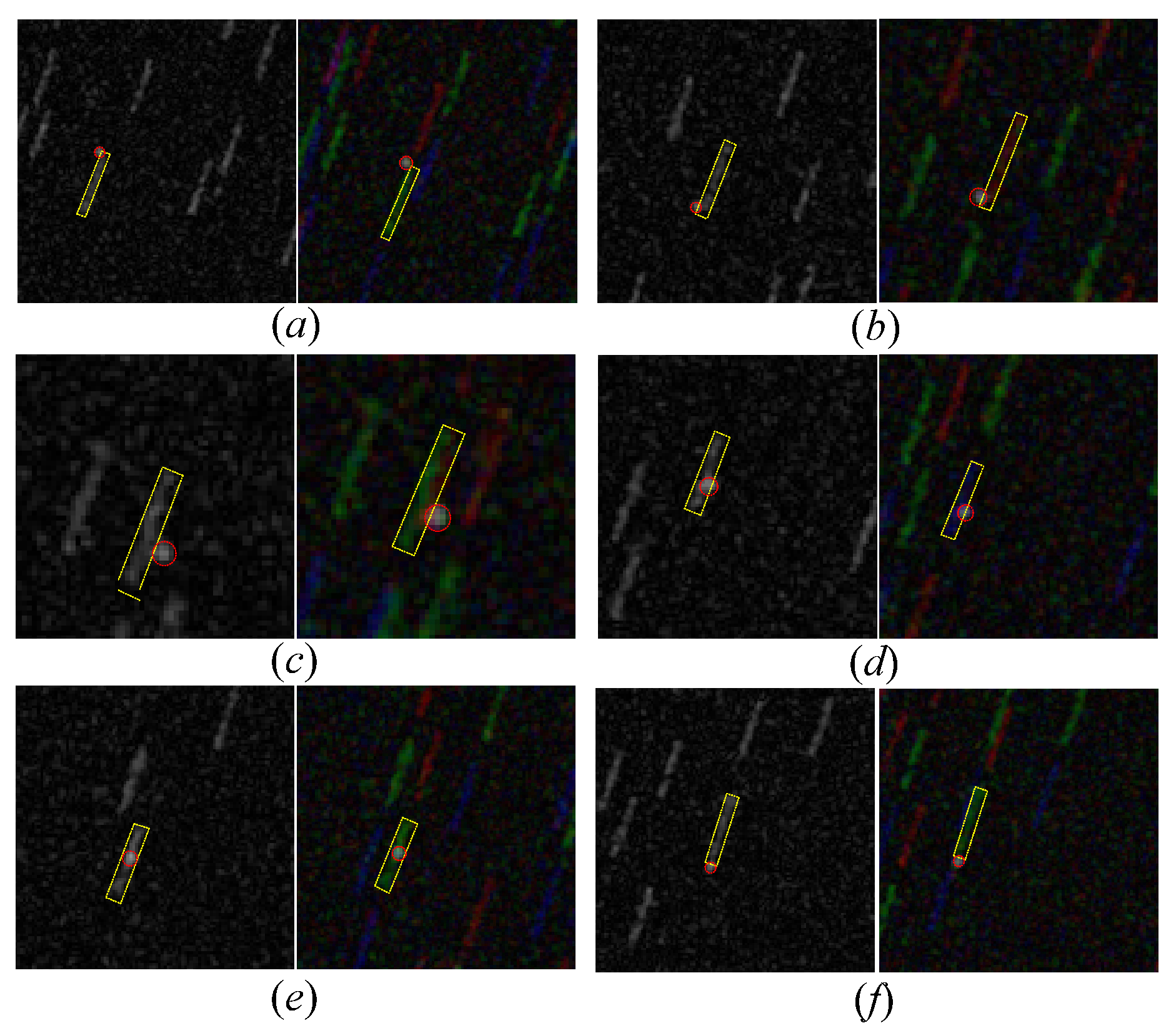
Figure 10 shows the common star trailing occlusion debris target scene, covering three types of occlusion cases. The left side of each scene shows a single gray image (a,c,e), and the right side shows three consecutive superimposed images (b,d,f).

Figure 11 shows the image features of the occluded fragment target. It can be seen that the gray features of the fragment target are quite different from the stellar trail. In case one, when the object is completely occluded, we can also distinguish it according to the continuous frame image. It can be seen that although there are feature differences in occlusion, there are fewer feature pixels, and it is difficult to detect quantitatively by noise interference, which makes it impossible to distinguish rules. Although the statistical distribution difference is obvious, the fragment target pixels are too few to be directly extracted according to the statistical distribution difference.

By focusing on these difficulties and problems, this section designs a small, fully connected convolutional network (FCN). By training the occluding fragment target samples, the edge “bulge” information after rectangular fitting is used as a suspected target for FCN calculation and finally determines whether it is a fragment target. The small FCN design is shown in

Table 2. Small FCN network architecture.

Stage	Convolutional Kernel	Inputs	Outputs
1	3 × 3 × 16	8 × 8 (×3) Note	8 × 8 × 16
2	3 × 3 × 16 × 32	8 × 8 × 16	8 × 8 × 32
3	3 × 3 × 32 × 64	8 × 8 × 32	4 × 4 × 64
4	3 × 3 × 64 × 128	4 × 4 × 64	2 × 2 × 128
5	3 × 3 × 128 × 256	2 × 2 × 128	1 × 1 × 256
6	1 × 256	1 × 1 × 256	1 × 1

Note: (×3) represents an extended network, used for continuous data input in the front and back three frames.

, which contains six layers of convolution calculation. The final output result 0 represents the non-fragmented target, and 1 represents the fragmented target.

2.4. Multi-Frame Association Tracking

A traditional multi-frame association mainly relies on inter-frame difference to achieve star background removal after registration. However, in long-tail scenes, especially when the SNR between stars and targets is low, it is difficult to eliminate the interference caused by noise after registration, which will seriously affect the correlation of fragmented targets. At the same time, due to the long tail, fragmented targets are easily obscured by the tail, resulting in the inability to continuously associate fragmented target information between multiple frames and causing tracking interruption.

In response to this issue, this section adopts a multi-frame suspected target detection based on a small FCN. Suspected “protruding” targets in three consecutive frames of images are put into the extended network in Table 2, and further association and confirmation of fragmented targets are completed through multiple frames to improve the accuracy of detection and tracking.

3. Engineering Implementation Framework

The algorithm presented in Section 2 mainly includes five parts: image contrast calculation, binary segmentation annotation, star trailing rectangle fitting, fragment target FCN identification, and inter-frame correlation. Among them, contrast calculation and binary segmentation annotation can be achieved through parallel pipeline computing based on digital logic and real-time processing of input data streams; Star trailing rectangle fitting uses digital logic-based rectangle parameter calculation and slice extraction acceleration; Fragment target FCN identification and inter-frame correlation are solved in real-time using DSP. This is also because in the staring fragment target mode, there are fewer targets in a “stationary” state, and DSP can be used to complete the calculation.

Figure 12 shows the calculation and testing block diagram. During the testing process, the simulated image data and instructions are sent through the upper computer of the PC. Sent to the FPGA of the hardware board through the network port, the image data are first stored in the cache after being parsed by the network communication protocol module, and instructions are used for module control. In FPGA, the contrast of the data cached in DDR is calculated, and the annotation of the Binary image and the rectangular fitting calculation of the star trail are completed. According to the rectangular fitting, the suspected fragment target with raised rectangular edges is sent to the DSP. The DSP judges the data reception based on the EMIF bus and performs FCN calculations to determine whether the target is true or false. Finally, inter-frame data association is completed in the DSP. At the same time, DSP serves as the main controller of the hardware, responsible for instruction parsing, telemetry generation, and module program scheduling of the entire system.

4. Experimental Results and Comparison

This section tests the algorithm, mainly including three items: accuracy of star/target detection based on Table 1 parameters; The relationship between the accuracy of star/target detection and the inter-frame interval Fi when SNR = 5; The relationship between the accuracy of star/target detection and the SNR when Fi = 50. Finally, a comparison of performance indicators was made between the test results and previous literature.

Star/debris targets for detecting and tracking based on 100 sets of simulation data are generated based on the parameters in Table 1. The total true value of the number of stars in the simulation is N(s, t), and the true value of the number of debris targets is N(d, t); The number of detected stars is N(s, d), and the number of fragment targets is N(d, d); The detected number of false alarms for stars is N(s, f), and the number of false alarms for debris targets is N(d, f); The number of missed stars is N(s, L), and the number of debris targets is N(d, L). Among them,

$$\left\{\begin{array}{c}{N}_{(s,t)}=N_{(s,d)}+N_{(s,L)}-N_{(s,f)}\\ N_{(d,t)}=N_{(d,d)}+N_{(d,L)}-N_{(d,f)}\end{array}\right.$$

(5)

Therefore, the precision P_s, recall R_c and F₁ are as:

$$\left\{\begin{array}{c}{P}_s=\frac{(N_{(s,d)}-N_{(s,f)})+(N_{(d,d)}-N_{(d,f)})}{N_{(s,d)}+N_{(d,d)}}\\ R_c=\frac{(N_{(s,d)}-N_{(s,f)})+(N_{(d,d)}-N_{(d,f)})}{(N_{(s,d)}+N_{(d,d)})+(N_{(s,L)}+N_{(d,L)})}\\ F_1=2\frac{P_s{R}_c}{P_s+R_c}\end{array}\right.$$

(6)

4.1. Accuracy of Star/Target Detection Based on Table 1 Parameters

Generate 100 sets of simulation data for algorithm simulation training, and test the other 100 sets of generated data based on Equations (5) and (6). Among the 100 sets of test data, there are a total number of N_{(s, t)} = 123417 stars, with N_{(s, d)} = 113219 detected stars, N_{(s, f)} = 10771 false alarms, and N_{(s, L)} = 20969 missed stars; debris N_{(d, t)} = 2000, detected debris N_{(s, d)} = 1764, false alarms N_{(d, f)} = 223, and missed debris N_{(d, L)} = 459. Obtain the precision and recall rates of stars and debris, as shown in

Table 3. Accuracy of star/target detection based on Table 1 parameters.

No.	Type	Precision Ps	Recall Rc	F1
1	Star	0.9049	0.7635	0.8282
2	Debris	0.8736	0.6932	0.7730
3	Star + Debris	0.9044	0.7623	0.8273

.

In 100 sets of generated test data, a total of 472 debris targets were occluded by stellar tails, including 108 targets in occlusion one, 229 targets in occlusion two, and 135 targets in occlusion three. Therefore, it can be estimated that in the simulation scenario based on Table 1, the target’s occlusion rate is 23.6%, the probability of complete occlusion (case one) is 5.4%, the probability of edge-to-tail contact (case three) is 6.75%, and the probability of occlusion below 1/3 (case two) is 11.45%. Considering that both scenario two and scenario three can detect targets through processing, 77.12% of the occluded targets can have a chance to be detected after processing.

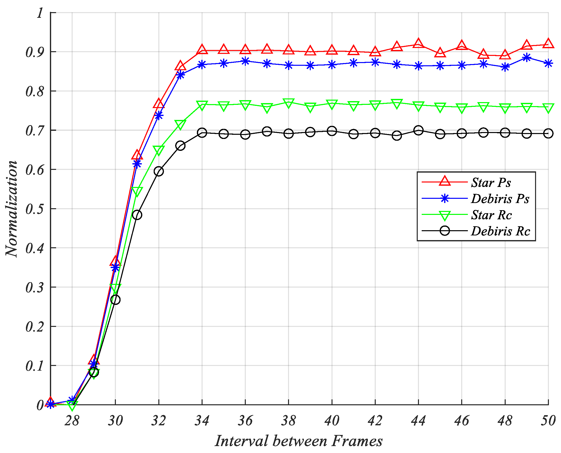
4.2. The Relationship between the Accuracy of Star/Target Detection and the Interval Time between Frames

The smaller the time interval between frames, the closer the minimum distance between the two images of star tails and the higher the density of tails in the entire image. When F_i = L_f, the debris target has a (L_d + 2W_f)/P_i = 55% chance of being obscured by the stellar tail, completely losing the possibility of successful detection. Therefore, studying the relationship between the accuracy of star/target detection and the inter-frame interval P_i is helpful for subsequent research on in-orbit imaging modes.

Based on the parameters in Table 1, the 100 × 24 sets of test data were generated with 24 types of F_i, where $F_i\in (L_f,50]$, $F_i\in Z^{+}$, for the precision and recall corresponding to the detection results of stars and debris, as in Figure 13.

When the interval between frames is less than 34, the duty cycle of the star trailing overlay image is 76%, making it difficult to accurately register and determine the star between two frames. Rectangle fitting detection is basically ineffective, and the accuracy rate drops sharply.

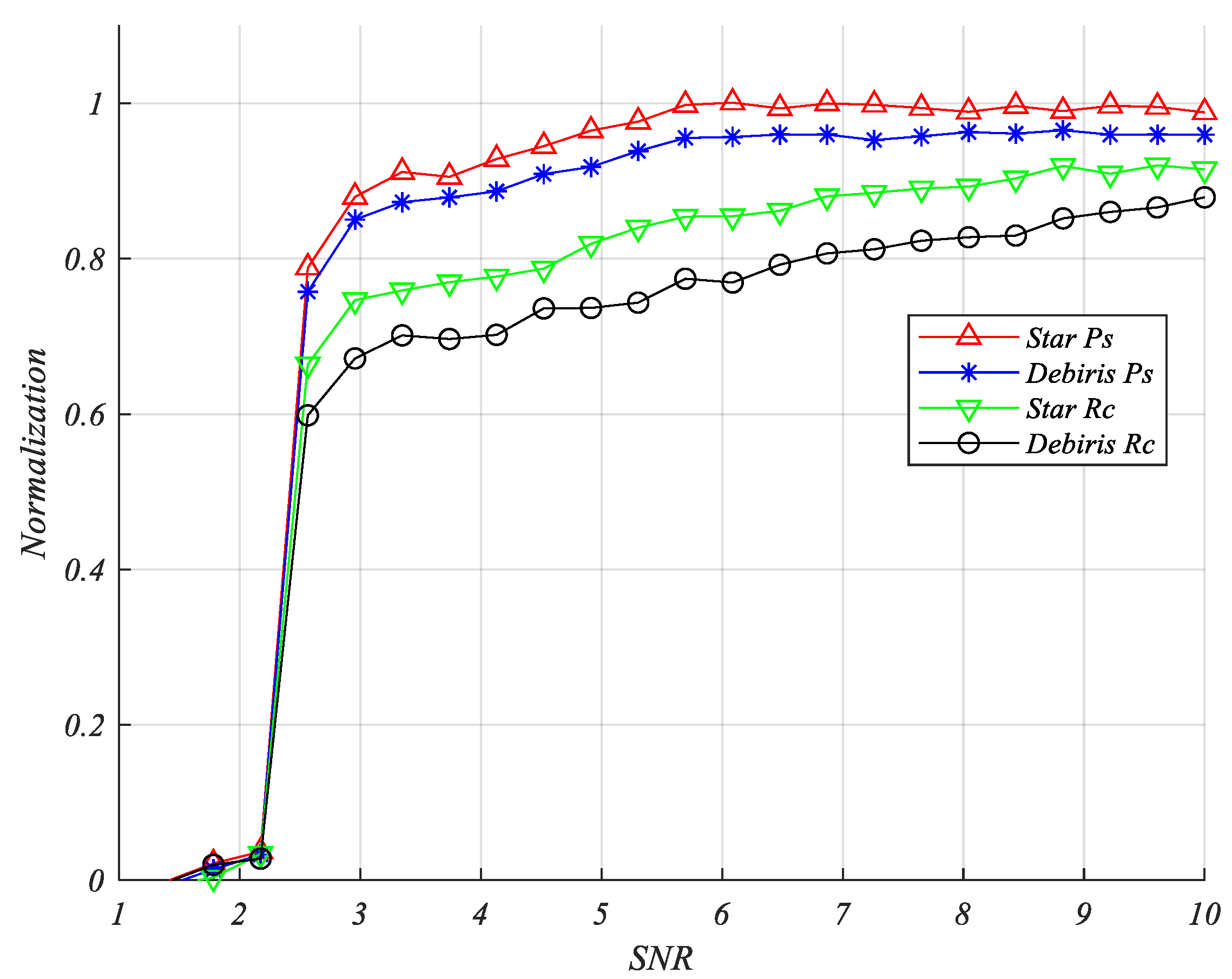
4.3. The Relationship between the Accuracy of Star/Target Detection and Signal-to-Noise Ratio

The SNR basically determines the detection accuracy. This section generates test data for different SNRs, conducts tests, and provides changes in detection accuracy. Based on the parameters in Table 1, the detection accuracy during statistics is shown in Figure 14.

When the SNR is less than five, the detection accuracy gradually decreases. By 2.5, the detection accuracy is greatly reduced due to the segmentation contrast threshold. By 1.4, it is basically impossible to detect stars and targets. At this time, the tail of stars is affected by noise, and the image is in a dispersed, fractured state, making it difficult to extract features through feature detection; When SNR > 6.5, the distinction between stellar trailing and debris target features is relatively clear, with almost no missed detections, and false alarms decrease as the SNR increases.

4.4. Comparison

Previous algorithms mainly focused on detection, tracking, and target feature extraction, relying mainly on traditional frame differences and correlations, making it difficult to apply to dim target detection in dense stellar long tail backgrounds. This section qualitatively compares the literature method with this method.

In

Table 4. Comparison with different literatures (×: unavailable; √: available).

No.	Methods	Low SNR	Occlusion Detection	Lightweight Computing	Continuous Tracking
1	[12]	×	×	×	√
2	[13]	√	×	√	×
3	[15]	√	×	×	√
4	[16]	√	×	√	×
5	[17]	√	×	×	×
6	[18]	√	×	×	√
7	[19]	√	×	√	√
8	Proposed	√	√	√	√

, previous literature mainly focused on detection and tracking under low SNR conditions. We conduct the rectangle contour fitting to the stellar tails, as the angle and length of the trailing star can be predicted. Then we obtain the image with the stellar tail, and the debris target superposed together, which can be analyzed in three cases. These images are put into the FCN, which can tell which case the images belong to, then we can obtain the information on the occluded faint debris target.

In this paper, under the condition of a detection accuracy of 90%, star and debris target detection were achieved in dense and long tail scenes, solving the problem of occlusion obstruction and continuous tracking caused by tail dragging under a high-duty cycle. When compared with previous algorithms, it has significant advantages.

5. Conclusions

This paper presents a detection method for staring debris targets in high-density star long-tail scenarios. By performing rectangular fitting on trailing stars, the influence of noise on the grayscale values of the trailing region was reduced. Based on the statistical characteristics of the staring targets, FCN was trained and learned to detect occluded targets. In total, 100 sets of 15 consecutive frames of images generated by simulation were tested, with a recall rate of over 90%. We conducted detection accuracy tests on changing inter-frame intervals and SNR and provided the relationship between indicator parameters and key parameters. When the inter-frame interval is less than 34, the detection accuracy begins to decrease; When the SNR is below 2.5, the detection accuracy drops sharply. Compared with previous literature, this design has the ability to detect and track occluded targets while ensuring an over 90% detection rate and a less than 10% false alarm rate simultaneously, effectively solving the problem of continuous tracking caused by target occlusion in previous methods.