Film Boiling around a Finite Size Cylindrical Specimen—A Transient Conjugate Heat Transfer Approach

Featured Application

Film boiling simulations were enabled without using powerful computational resources on relatively large-scale domains, thereby preserving the important features of flow by using a DNS of interface motion, confirmed by comparison with a snapshot from an experimental investigation.

Abstract

The DNS of film boiling requires strong computational resources that are difficult to obtain for daily CFD use by expert practitioners of industrial R&D. On the other hand, film boiling experiments are associated with the usage of expensive and highly sophisticated apparatus, and research to this end is relatively difficult due to high heat flow rates that are present in the process itself. When combined with transient heat conduction in a solid, the problem becomes significantly difficult. Therefore, a novel method in computation of conjugate heat transfer during film boiling in a quiescent liquid is proposed in this paper. The method relies on the solution of mass, momentum and energy conservation equations in a two-fluid framework, supplemented with the appropriate closures. Furthermore, turbulent flow was determined as an important parameter in obtaining an accurate solution to temperature field evolution in a solid specimen, via the proper modeling of the turbulent kinetic energy (TKE) value, that was imposed as a constant value, i.e., the frozen turbulence approach. It was found, in addition, that the appropriate TKE value can be obtained by use of Kelvin–Helmholtz instability theory in conjunction with boundary layer theory. The obtained results show excellent agreement with the experimental data within the first 15 s of the experiment, i.e., the first ca. 10% of the total duration of the film boiling mode of heat transfer. Furthermore, the heat transfer coefficient matched the error bands prescribed by the authors of this paper, which presented the correlations, whilst the averaged values are far beyond this band, i.e., are slightly more than 30% higher. Further inspection revealed a measure of similarity between the computational result of the volume fraction field distribution and the experiment, thus confirming the capability of the method to obtain realistic interface evolution in time. The method shows full capability for further pursuing industrial-scale film boiling problems that involve turbulent flow and the conjugate heat transfer approach.

1. Introduction

The sustainable development of the world’s leading economies is strongly linked with optimized power engineering and metal processing industries. However, it is less known that these two industrial branches require well-optimized processes, which involve boiling phenomena, to operate smoothly. Thus, the nucleate boiling regime is preferred among thermal power plants, since it allows for the removal of high heat fluxes with relatively small temperature differences on the heat transfer surface. Exceeding this limit, i.e., by surface overheating, may lead to a failure of the system with catastrophic consequences. This is the so-called film boiling regime. However, this unfavorable boiling mode in power plants is very common in the metallurgical quenching process, that is, the rapid cooling of a metal object to achieve certain microstructure that yields desired mechanical properties of the same, for example, hardness. To this end, a comprehensive set of experimental data is needed to achieve the safe and environmentally friendly work of these plants. But this experimental work is very costly and should be preceded by comprehensive theoretical and computational studies to extract the benefit from it. However, computational studies of boiling incorporate very resource-demanding interface tracking methods (ITMs), which require very fine grid resolutions to model the interfacial phenomena, well known as single-fluid methods, such as, for example, volume-of-fluid (VOF), coupled with direct numerical simulation (DNS) of interface motion, in which the volume fraction of vapor/liquid is tracked by solving the advection equation. On the other hand, two-fluid methods can overcome this but require adequate closure models. Compared to the aforementioned single-fluid models, a two-fluid model is considered to be able to predict more accurate results on coarser mesh, owing to the necessity of resolving the interface geometry/shape, though two sets of momentum and energy equations that must be solved. However, due to the averaging process in the formulation of the governing equations, the shape and area of the liquid–vapor interface are lost, and the dynamics related to the interface, e.g., surface tension and interphase forces, cannot be directly computed.

Relevant fundamental studies refer to investigations that are focused more on microscopic phenomena and can be used for validation or verification purposes. The mass transfer model based on the energy jump condition at the interface can be found in a study by Nichita [1]. The model is implemented within ANSYS Fluent as a part of a coupled level set and volume-of-fluid (CLSVOF) approach in the set of governing equations method via the source term in mass and energy conservation equations. The slug flow in a microchannel was studied by Magnini [2]. The considered cases include isothermal flows: flows with heat transfer and flows with phase change, that is, evaporative flows. The commercial software ANSYS (https://www.ansys.com/) Fluent was extended in the direction of curvature calculation in the computation of surface tension body force in a single-fluid VOF model. To this end, a height function algorithm was implemented within the software and validated against the already available interface reconstruction algorithm in the software. Furthermore, an evaporation model was also included; however, since the method is aimed at microscale simulations, the assumption of thermodynamic equilibrium at the interface does not hold anymore, that is, the temperature of the interface differs from the saturation temperature. Another modified formulation of the energy jump mass transfer model and its application in relevant film boiling studies was proposed by Sun et al. [3]. The model was applied in solution to a one-dimensional Stefan problem and film boiling on a horizontal surface, thereby assuming the coexistence of saturated and unsaturated phases in the domain. The usage of the instantaneous level set method (LSM) in conjunction with the stabilized finite element method (FEM) in the numerical modeling of the quenching process was proposed by Kosseifi [4]. The proposed model used the variational multiscale (VMS), which has been claimed as an method analogous to large eddy simulations (LES). The performed numerical simulations demonstrated the method’s capability in resolving the vapor film and the obtained solid temperatures were compared with experimental data. A mass conservative method for the computation of phase change processes using a sharp interface representation was proposed by Sato and Ničeno [5]. The mass transfer rate was computed directly from the heat flux at the interface, thus allowing for the sharp distribution of the dominant mass transfer rate in the interface region; the interface thereby being denoted as an isosurface (isoline in 2D) of the phase indicator (color function) equal to 0.5, and the cells bisected by this surface being marked as interface cells. In the evaluation of temperature gradients, the orthogonal distances between the center of the interface cell and the interface were used. A study on film boiling in the vicinity of a sphere immersed in saturated water at atmospheric pressure, also considering a case with the involved radiation heat transfer, was carried out by Arévalo et al. [6]. Film boiling was studied for various solid surface temperatures, and the obtained heat flux values were compared with results obtained using different correlations. Furthermore, an estimation of radiation coupling factors was performed using numerical simulation. A comprehensive review of computational models for the simulation of boiling and condensation phenomena was presented by Kharangate and Mudawar [7]. Among the reviewed models, three distinct mass transfer models were outlined, namely: the energy jump, Schrage, and Lee models, and their characteristics were summarized in tabular form. It should be noted that only the energy jump mass transfer model, among the three presented models, stems from basic principles, i.e., it does not require any empirical input to estimate the mass transfer across the interface. On the other hand, it requires an initial vapor cell to induce mass transfer, thus being incompatible for bulk boiling simulations. An exception to this general rule was found by Chen et al. [8], wherein the local cell size and gradient of the volume field were involved in the Lee mass transfer model. A study of the pool boiling process in which a film boiling regime was achieved as a consequence of exceeding the critical heat flux (CHF) limit was carried out by Sato and Ničeno [9]. The authors used the aforementioned approach [5] for handling multiphase flow with a phase change in an Eulerian framework, that is, using a single set of governing equations with a color function as an interface indicator, but adapting it to turbulent flow modeling using a large eddy simulation (LES) approach. More recently, the simulation of the dispersed flow film boiling (DFFB) regime using the level set method (LSM) in conjunction with direct numerical simulation (DNS) of turbulence was presented by Saini and Bolotnov [10]. This adiabatic flow study was carried out using “in-house” computational software PHASTA (https://docs.cci.rpi.edu/software/PHASTA/), based on the stabilized finite element method, with conditions at the inlet obtained using single-phase computation. More recent studies involved the Lee model’s application in modeling of film boiling around a horizontal cylinder, such as that presented by Wang et al. [11].

In summary, fundamental studies have revealed the main issues regarding mass transfer modeling, and demonstrated the main mass transfer models; among them, the energy balance model has been identified as the most prominent, since it does not rely on empirical constants and stems from pure energy balance at the interface between the fluids. The two main issues in successful resolution of film boiling during immersion quenching using this model are:

• Reconstruction of the temperature gradient at the vapor–liquid interface in the mass transfer model.
• Adequate turbulence modeling.

The necessary prerequisite to this end (first item) is the existence of the identifiable interface between the phases, such that mass transfer may take place at the interface. This is due to the gradient of volume fraction incorporated in the computation of interfacial area density. Furthermore, an additional remark must be pointed out regarding turbulence modeling (second item), since the turbulent heat flux is defined by consideration of the effective thermal conductivity and has to be computed accurately in order to estimate the transient temperature distribution in a solid object correctly. Hence, more elaborate turbulence modeling has to be carried out, since there is a complex interaction between the vapor and liquid phases in the process. However, these approaches are mostly assigned to one-fluid formulations, such as VOF or LSM, wherein a single set of governing equations is solved for both phases, and hence individual phase modeling, instead of their mixture, becomes difficult to handle.

Therefore, in this paper, a novel method for the estimation of mass transfer across the interface in a thermally driven phase change process is presented. The method is implemented within a two-fluid VOF formulation (available in the commercial CFD software ANSYS Fluent). It consolidates the benefits of the two multiscale multiphase modeling approaches—low-resolution meshes and large time steps from the two-fluid formulation—whilst preserving the sharp interface treatment using a geometrical reconstruction algorithm, that is, a property of the pure VOF method, generally used for DNS of interface motion. The strong point of the proposed mass transfer estimation method is in the energy jump model inherited in the final model, thus relying completely on basic principles when mass transfer across the interface is considered. Furthermore, in the usage of asymptotic-like behavior of the two-fluid model via the appropriate source terms in mass (zero-resistance), momentum (anisotropic drag) and energy equations, low-resolution computational meshes may be used whilst still preserving all the necessary features of a single-fluid model in a manner that interface geometry may be tracked.

The novelty/gap to be filled is in consideration of a standard DNS of interface motion case within the two-fluid VOF framework, thus making large-scale computations less computationally demanding. In doing so, hybrid meshes may also be applied, thus alleviating the need for structured or hexahedral (quadrangular) meshes. More details on how this is accomplished using the present approach are presented in the remainder of the paper.

2. Materials and Methods

2.1. Description of the Experiment

A film boiling experiment in the case of saturated and subcooled bath medium reported by Momoki et al. [12] was used as a validation study in this work. Specimens of different sizes were submerged in liquid coolant and the temperature distribution was measured at the specimen’s center. The specimens were made of silver; thus, due to small Biot number, that is, 0 < Bi < 0.1, a lumped transient heat conduction model was relevant for estimation of solid temperature due to inexistence of significant temperature gradients with respect to space coordinates of the solid body. A sheathed K-type thermocouple was placed at the center of the specimen, and the sampling time was 0.25 s.

In the context of the present work, a cylinder specimen with dimensions 45 mm diameter and 45 mm length, for which transient temperature distribution was available, was used as a validation benchmark. Specimens made of materials without structural transformation during the process were used for determination of cooling characteristics of a quenchant medium. The selected geometry model was taken due to availability of the measured temperature data at the center of the specimen.

2.2. Mathematical Modeling

The mathematical model that underlies the proposed computational method was composed of mass, momentum and energy conservation equations, written on a per-phase basis and supplemented with adequate closure models. A full description of the governing equation set, and appropriate closures is provided in [13], whilst special attention regarding the heat transfer modeling at the interface is presented herein. The goal was to invoke the kind of asymptotic-like behavior of a two-fluid model, in a sense that a sharp interface was maintained between the phases, whilst preserving all the features of a two-fluid model, i.e., relatively small mesh resolutions with relatively high time steps. In what follows, a brief overview of the heat transfer aspect of the model is presented together with the turbulence modeling issues.

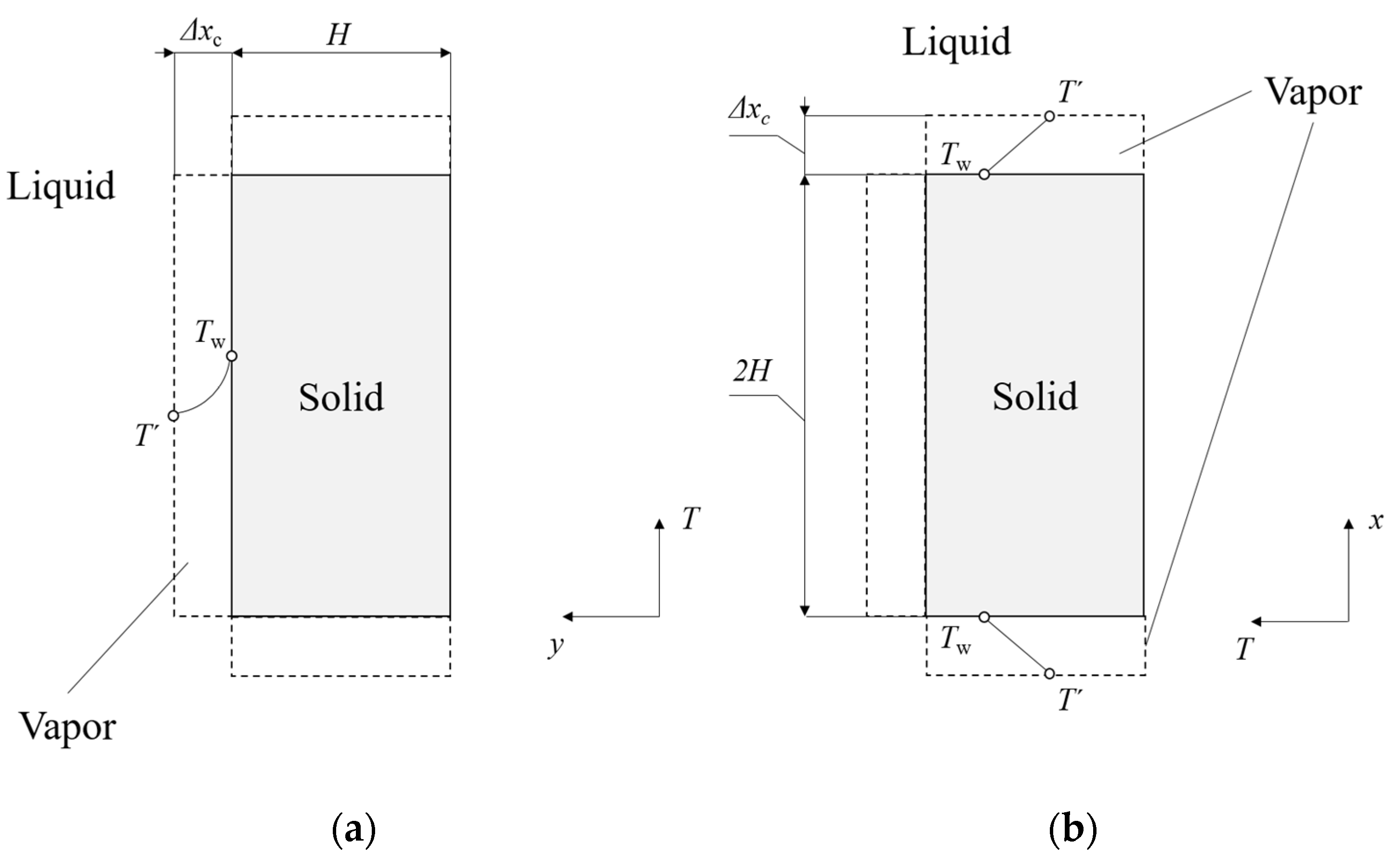
2.2.1. Interphase Heat Transfer

Since the saturation temperature liquid was assumed at this point, i.e., $T^{\prime }=T_l$, and the heat flow rate from the interface to the liquid phase reduces to ${\Phi }_l=h_l A_i \left( T^{\prime }-T_l\right)-\dot{m_{lv}}{h}^{\prime }=\dot{m_{lv}} h^{\prime }$, the volumetric heat flow rate from the interface to the vapor phase reads

$${\Phi }_l=h_l{A}_i\left(T^{\prime }-T_l\right)-{\dot{m}}_{lv}{h}^{\prime }=-{\dot{m}}_{lv}{h}^{\prime }$$

(1)

$${\Phi }_v=h_v{A}_i\left(T^{\prime }-T_v\right)+{\dot{m}}_{lv}h{″}^{}$$

(2)

where h_v is the heat transfer coefficient at the vapor side of the interface, h′ is the specific enthalpy of a saturated liquid at the system pressure, $A_i$ is the interfacial area density, $T^{\prime }-T_v$ is the temperature difference between the interface and the vapor phase, ${\dot{m}}_{lv}$ is the volumetric mass transfer rate for a vapor–liquid phase pair in a phase change process, and h″ is the enthalpy of the saturated vapor at the system pressure. It is noteworthy that a heat balance between the phases exists, i.e., ∣Φ_v∣ = ∣Φ_l∣. The heat transfer coefficient at the vapor phase of the interface has a fictitious function in a sense that is used to involve the approximated distance between the neighboring cell’s center to the interface and thus to approximate the temperature gradient in the vicinity of an interface.

2.2.2. Turbulent Flow

By insertion of average turbulent kinetic energy in all the cells except the ones in the immediate neighborhood of the heat transfer surface, i.e., the specimen surface’s adjacent cells, one may enhance the heat extraction from the solid and thus achieve better agreement with the experimental data. This is due to the enhanced heat flux at the interface that reads [7]

$$\overrightarrow{q_n}=\left(\lambda +{\lambda }_t\right)\frac{\partial T}{\partial \overrightarrow{n}},$$

(3)

where λ is molecular thermal conductivity, λ_t is the turbulent thermal conductivity, and $\frac{\partial T}{\partial \overrightarrow{n}}$ is the temperature gradient in the normal direction of the interface. Joining together molecular and turbulent thermal conductivity gives effective thermal conductivity

$${\lambda }_{eff}=\lambda +{\lambda }_t.$$

(4)

In the validation case, the flow is considered turbulent, although the turbulence transport equations are not solved; yet, the turbulent kinetic energy (TKE) is prescribed in all the cells of the computational domain, thus affecting the turbulent dynamic viscosity, μ_t, and, correspondingly, the turbulent thermal conductivity.

The turbulent viscosity is directly proportional to the square of turbulent kinetic energy, ${\mu }_t \propto TK{E}^2$, and is involved in computation of effective thermal conductivity, Equation (4). While the molecular thermal conductivity is a well-known physical property of a continuum, the turbulent thermal conductivity is computed analogously to the molecular Prandtl number, using the turbulent Prandtl number, $P{r}_t={\mu }_t{c}_p/{\lambda }_t$, that is taken as constant, 0.85, in the present research. The turbulent viscosity is modeled as in standard realizable k-ε models, using a variable factor C_μ; thereby, the dissipation rate is kept as the default value.

This approach can be referred to as the “frozen turbulence” approach, since the governing equations of turbulent transport are not solved, yet the turbulent kinetic energy contributions to the effective thermal conductivity, and thus the heat flow rate extraction from the solid specimen, are considered by prescription of TKE values thorough the domain.

Furthermore, a dispersed phase (vapor phase) formulation of a realizable k-ε turbulence model is chosen for the computations herein. Thus, only the bulk phase turbulence is modeled with transport equations (that are not solved in the present case—a frozen turbulence approach), while dispersed phase turbulence modeling is carried out using the Tchen correlation [14].

To sum up, in this paper, we simulated the temperature evolution in a solid material during the film boiling phase while cooling the material in a liquid pool. To do so, we needed to appropriately model the mass transfer at the vapor–liquid interface. Since the molecular thermal conductivity is not the only one present in the heat balance at the vapor–liquid interface, we needed to inject the turbulent thermal conductivity that has a significant influence on the heat transfer from the specimen to the bulk fluid. To accomplish this, due to instabilities associated with the application of the RANS model during the process, we were forced to mimic the turbulence modeling by involvement of only the turbulent kinetic energy as the input parameter but yielding the variable turbulent viscosity due to flow-dependent $C_{\mu }$ factor that is present in the realizable k-ε models in contrast to the standard or RNG models that have this factor as a constant. Further treatises on the so-called frozen turbulence approach are shown in the next subsection of this paper.

2.2.3. The “Frozen Turbulence” Approach

The half of the sum of principal stresses in a nonlinear Reynolds stress tensor, which appears in momentum conservation equation after the Reynolds averaging of dependent variables is applied due to fluctuations in these quantities in a wide spectrum of wavelengths and frequencies, forms the turbulent kinetic energy—see, e.g., Markatos [15]—as follows:

$$TKE=\frac{1}{2}\underset{¯}{{v^{\prime }}_i{v^{\prime }}_i},$$

(5)

where ${v^{\prime }}_i$ is the fluctuating velocity component in the i-th direction (index notation). Hence, the turbulent kinetic energy is strongly interlinked with another flow variable, the turbulent viscosity, ν_t, that is relevant only for turbulent flow. Since it appears in the effective thermal conductivity term, heat rejection from a cylinder specimen is thus plausible. An analogy between film flow and free jet flow near the nozzle exit can be made, since the initial core with a laminar flow inside precedes the disturbed flow. The disturbance that appears in a downstream direction is a Kelvin–Helmholtz instability and is, according to Hoppe and Breurer [16], a consequence of different tangential velocities across the interface between two fluids; disturbance of this type is due to surface instabilities, and is noticeable in the case of large bubbles wherein the significant influence has surface tension in contrast to small bubbles of small radii. The turbulent kinetic energy is, furthermore, in close relationship with turbulence intensity, another measure of turbulent flow. An experimental work by Philip [17] revealed that, in the case of annular jet flow, the peaks of turbulence intensities appear in the shear layers; thus, as claimed by the author, turbulence occurs in the shear layers. A study by Kimber [18] revealed that turbulence intensity profile closely follows the TKE distribution in a single jet flow. It is the bubble induced turbulence (BIT), studied in Ničeno et al. [19], wherein the liquid flow is turbulent, whilst the flow inside the vapor phase is laminar. Another analogy is the flow of breaking sea waves in the surf zone; studies by Kashima et al. [20] and Mori et al. [21] provide more detail in this regard, while the numerical assessment of this topic was presented in a simulation by Makris et al. [22]. The authors conducted a detailed study using a Lagrangian method that corresponds to the LES approach.

As per Cascioli et al. [23], in the co-flow of a jet, a strong shear between the jet and surrounding fluid domain contributes to turbulent kinetic production; on the other hand, the overall heat transfer rate, extracted from the solid object and transferred to the vapor–liquid interface, is significantly dependent on flow condition, i.e., the shear force driving the flow of liquid in the immediate neighborhood of the interface, as can be concluded from theoretical exposure provided by Sakurai et al. [24].

As in the case of jet or liquid film flow, in film boiling around a vertical cylinder, two distinct zones are defined according to Momoki et al. [12]: the zone of smooth interface and the zone where the interface is wavy. In contrast to flow of liquid film, which can be represented as Couette flow, as shown in Javed et al. [25], or flow film boiling, where the maximum velocity, regarding the film, is in the vicinity of the upper part of the film; in this case, i.e., the film boiling in a liquid pool, a more convenient approximation is a pipe flow, that is, a nonslip condition on the outer surface of the film.

In summary, frozen turbulence is applied throughout the domain by imposing constant TKE values: 0.25 m²/s² throughout the complete domain except for the initial cell layer in the vicinity of the specimen, wherein a zero value is imposed. This is shown in Figure 1, whereby only the enlarged zone next to the specimen has this zero value, while the remainder of the domain is filled with a TKE value of 0.25 m²/s². However, due to the application of a realizable k-ε turbulence model, which has a C_μ factor that varies throughout the domain, based on the flow field, the turbulent viscosity also tends to vary.

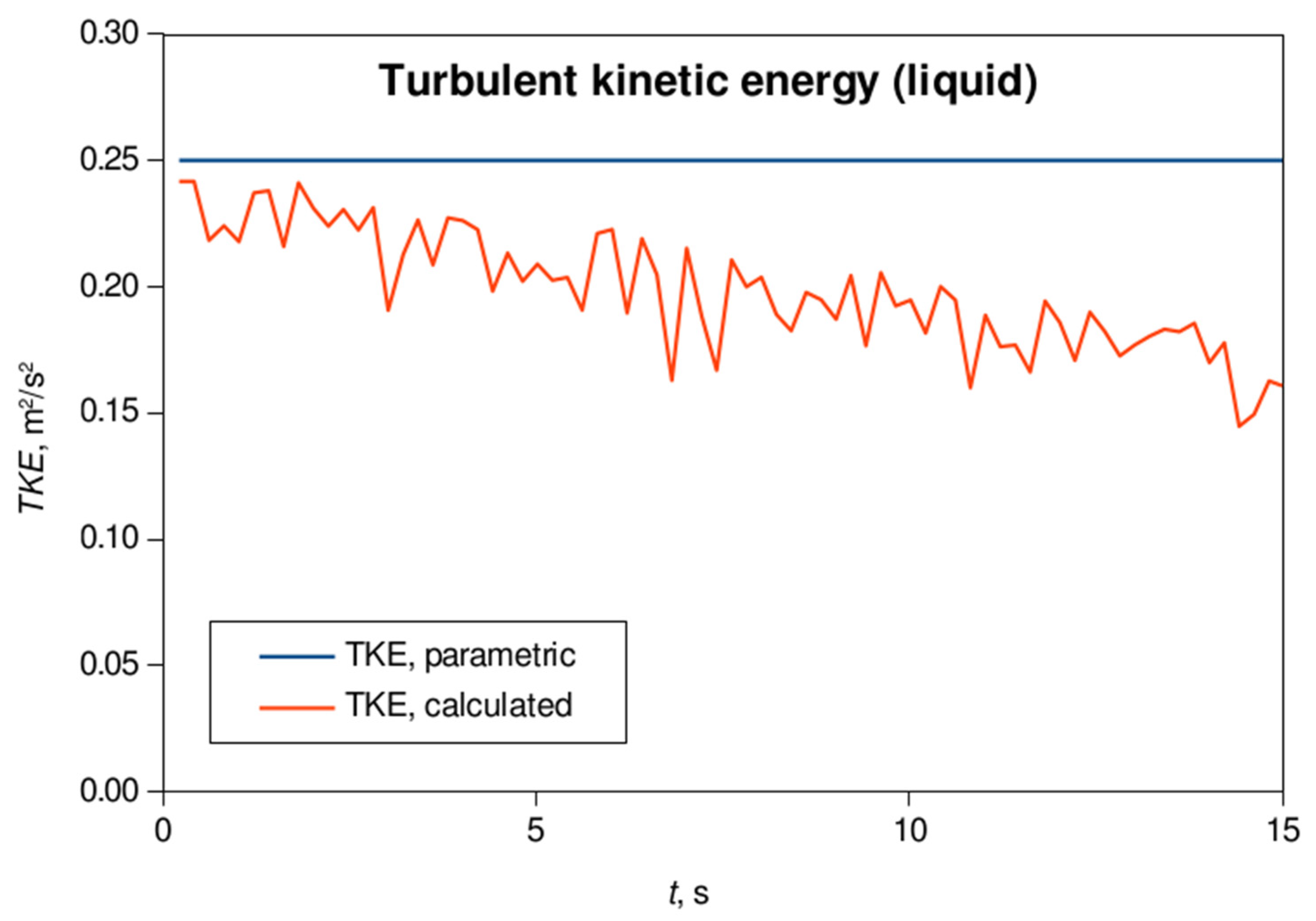
2.2.4. The Estimation of the Turbulent Kinetic Energy Value

It is interesting to note, however, that these values correspond to a great extent to the ones obtained with the equation for turbulent kinetic energy proposed in Hillier et al. [26] that, in the context of the present research, read

$$TKE\propto \frac{1}{4}{\rho }_{mix}\frac{\Delta w_{rel}{}^2{\left(F_v{F}_l\right)}^{\frac{1}{2}}}{{\left(\sqrt{F_v}+\sqrt{F_l}\right)}^2},$$

(6)

where ${\rho }_{mix}$ is the mixture density, Δw_rel is the relative velocity difference across the layer and F_v and F_l are the ratios between the density of vapor or liquid, respectively, and the sum of phase densities. The mixture density, ${\rho }_{mix}$, is defined as

$${\rho }_{mix}={\left({\rho }_v{\rho }_l\right)}^{\frac{1}{2}};$$

(7)

whilst density ratios F_v and F_l read

$$F_v=\frac{{\rho }_v}{{\rho }_v+{\rho }_l};$$

(8)

$$F_l=\frac{{\rho }_l}{{\rho }_v+{\rho }_l}.$$

(9)

The velocity profile in the case of immersion quenching has, at least to a certain extent, a parabolic-like profile; thus, an assumption of Poiseuille’s flow may be applied in obtaining the velocity distribution across the vapor layer, thereby assuming that the flow inside the layer is laminar, that is, λ_eff = λ. This assumption is justified such that, in the case of pool film boiling around a vertical surface of a cylinder, no-slip conditions at the interface between vapor and liquid, and the stationary wall of the cylinder are satisfied. Hence, a parabolic-like profile, as in the case of pipe flow velocity, may be considered.

The relative velocity, that is, the velocity input in the above expression, has to reflect the velocities in both the phases; hence, we assume that liquid velocity is zero due to pool boiling conditions; thus, the stationary interface between the phases may be assumed: the so-called “no-slip” condition. Consequently, inside the vapor film, a parabolic velocity profile may be assumed, which spreads over the vapor layer of thickness δ; hence, an averaged velocity through the vapor film is used in estimation of TKE, calculated from the continuity equation, that is, the mass conservation law, as follows:

$$\underset{\_}{w}=\frac{q_m}{{\rho }_v{\underset{\_}{\delta }}_m\pi }$$

(10)

where q_m is the mass flow rate per unit circumference, ${\rho }_v$ is vapor phase density, and ${\underset{\_}{\delta }}_m$ is an average thickness of the vapor layer, calculated as shown in Appendix A.

The computational model for analysis of the heat transfer phenomena during film boiling on a vertical surface was proposed by Yamada et al. [27], being derived for the case of film boiling on the vertical plane surface. Hence, a rectification of the unit width is conducted here by multiplication with π, when a cross-section of fluid element perpendicular to the flow direction is considered in obtaining the average velocity, Equation (10). The authors in the aforementioned article distinguish four different cases at the vapor–liquid interface, thereby considering the conditions at the bottom horizontal surface of the cylinder; hence, a no-slip condition at both the vapor layer beneath the cylinder and at the vertical surface is taken into account in this study due to the pool boiling conditions that are present in the flow.

The mass flow rate is defined analogously to Nusselt’s film condensation theory, from the momentum balance on the fluid element, with the exception of multiplication by 1/12 instead of 1/3. (The multiplication of the r.h.s. terms with 1/3 is also in the case with film boiling when slip, i.e., zero velocity gradient, is present at the top of the boundary layer, as shown in Yamada et al. [27].)

$$q_m=\frac{{\rho }_v \left({\rho }_l-{\rho }_v\right)g}{12 {\mu }_{v }}{\left({\underset{\_}{\delta }}_m\right)}^3,$$

(11)

where local layer thickness, present in the original model, is replaced with the averaged one, computed as shown in Appendix A.

The assumption of laminar flow inside the vapor layer may be approved with calculation of Reynolds number:

$$Re=\frac{\underset{¯}{w }{d}_{eqv}}{{\nu }_v},$$

(12)

where $\underset{\_}{w}$ is the mean velocity of the vapor phase, d_eqv is the equivalent diameter and ν_v is the vapor phase’s kinematic viscosity. The equivalent diameter is calculated as a difference between the outer diameter of the vapor film, i.e., D_v = d + 2δ, and diameter of cylinder, d = 0.045 m; or the equivalent diameter can be calculated as d_eqv = 4A/O = 2δ. This yields a value of 33.3 and thus confirms the accepted assumption of laminar flow inside the vapor film. The film boiling in the estimation of Reynolds number is considered with smooth interface between vapor and liquid, as in the study by Yamada et al. [27]. This very low value is a consequence of very small vapor film thickness, and a vapor velocity (volume averaged) in the range from ca. 1 m/s to ca. 1.3 m/s, that yields this low Reynolds number.

2.3. Computational Modeling

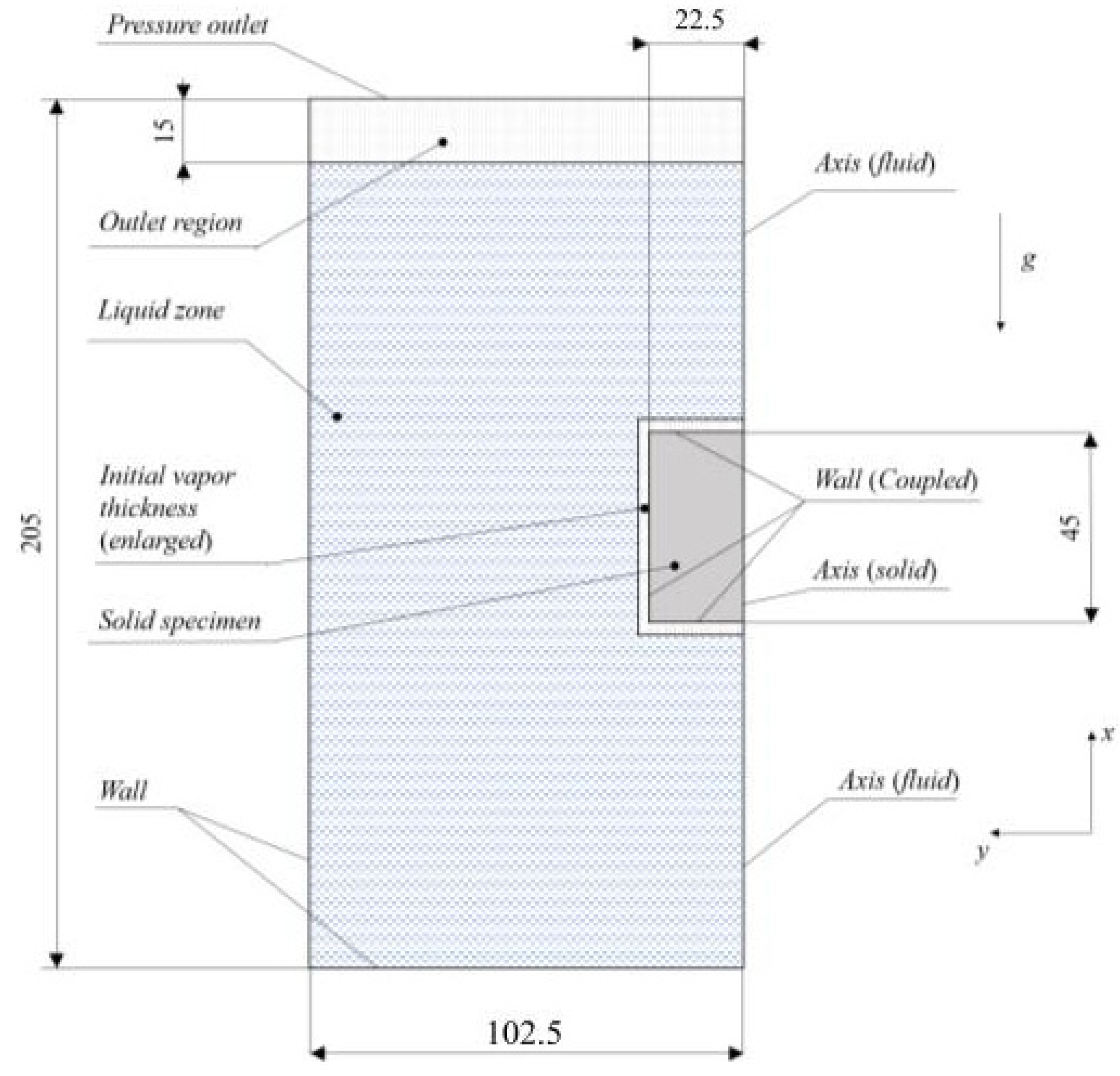
2.3.1. Description of the Case and Geometry

An axis-symmetric domain was constructed with the cylinder specimen placed in the middle of the domain’s height, as shown in Figure 1. The computational domain spans over the area x ∈ [−1.025 × 10⁻¹, 1.025 × 10⁻¹] m × y ∈ [0, 1.025 × 10⁻¹] m, and is composed of a fluid and solid part, separated via the fluid–solid interface. At the domain top, a 15 mm high outlet region is prescribed, containing the vapor phase. In the vicinity of the solid specimen, a one-cell vapor layer was initially placed, with a thickness of 0.61 mm, required for the mass transfer model in order to induce mass transfer. In Figure 1, the vapor blanked is, for the sake of simplicity, enlarged.

The domain is composed of 7938 quadrilateral cells (Figure 2a), with the refined cell zone adjacent to the specimen surface (Figure 2b). The specimen is made of silver and has equal diameter and height, 45 mm. The convergence of the equations is as follows: the residuals of the continuity equation were found to be of order 1 × 10⁻³; the x- and y-momentum conservation equations of the liquid phase were found to be of order 1 × 10⁻⁵ and 1 × 10⁻⁶, respectively, whilst the same equations yielded the residuals of order 1 × 10⁻⁵, x-momentum, and 1 × 10⁻⁶, y-momentum, in the case of the vapor phase; the energy equation residuals were reported to be less than 1 × 10⁻²⁰ for both the phases. The grid sensitivity check, however, was not performed according to findings in Gauss et al. [28], wherein it was shown that, when a two-fluid framework is used, the computational result is not dependent on the mesh resolution, as in the case of a single-fluid VOF method.

2.3.2. Boundary Conditions

The boundary conditions are assigned to the domain’s top, bottom and left side surface for both the phases, whilst the domain symmetry axis is defined as “axis” in the applied software. Thus, the top of the domain was set to the pressure outlet condition, with a prescribed outlet temperature 100 °C for both phases and the unit backflow vapor volume fraction. The bottom and left surface are defined as solid walls. The specimen surface is composed of three walls that interact with the fluid region via “coupled” condition.

2.3.3. Initial Conditions

The initial conditions involve the initial distributions of phase volume fractions, temperatures and velocities, supplemented with the initial profile of turbulent kinetic energy, that is, in contrast to other aforementioned dependent variables, maintained constant through the simulation, since the turbulence equations are not solved—the so-called “frozen turbulence” approach. The velocity fields of both phases were initially set to zero elsewhere in the domain, although the turbulent kinetic energy was initially set to a nonzero value everywhere except the initial vapor layer.

The initial temperature of a solid specimen is set to 600 °C, as per the experiment in Momoki et al. [12]. The liquid and outlet zone were set to the initial temperature of 100 °C. Inside the vapor layer, an initial temperature field is prescribed as follows (see Figure 3 and Figure 4):

In radial direction along the cylinder’s height, due to the analytical solution of the heat conduction equation in the radial direction of a cylindrical coordinate system (see Figure 3a for a qualitative description), a logarithmic temperature profile is imposed as follows:

$$T_{cell,i}=\frac{T^{\prime }-T_w}{ln\frac{H+\mathsf{\Delta }{x}_c}{H}}ln\frac{y_{c,i}}{H}+T_w,$$

(13)

whilst in the axial direction, at top and bottom surfaces, respectively, it follows the linear law due to the same reason as in the former case (the analytical solution to heat conduction PDE in the axial directions of the cylindrical coordinate system; see Figure 3b for a qualitative description):

$$T_{c,i}=\frac{T^{\prime }-T_w}{\mathsf{\Delta }{x}_c}\left(x_{c,i}-H\right)+T_w;$$

(14)

$$T_{c,i}=\frac{T^{\prime }-T_w}{-\mathsf{\Delta }{x}_c}\left(x_{c,i}+H\right)+T_w.$$

(15)

The edge element, however, is filled with the initial temperature computed as (Figure 4)

$$T_{c,e}=\frac{T_{ln}+T_{lin}+2T^{\prime }}{4},$$

(16)

which stems from an energy balance on a knot in the cell center, thereby assuming that the face temperatures of neighboring cells are those of their respective cell centers. This yields, however, the initial temperature in the edge control volume (CV) that is lower than these other two temperatures due to cooling contributions from two sides that remain at significantly lower saturation temperature.

2.3.4. Time-Stepping Procedure Applied in the Simulation

The time step applied in simulation is divided into two parts. Firstly, ten time steps with a size of 1 × 10⁻⁶ s were carried out. Then, a 2 × 10⁻⁴ s time step size was applied in the remainder of the simulation. Extensive study on the applied time-step size, and a brief comment on the applied equation discretization techniques can be found in [13].

3. Results

3.1. Temperature Distribution

The temperature distribution in a solid specimen agrees well with the experimental data by Momoki et al. [12] in approximately ten percent of the total film boiling period (the inflection point may be regarded as t ~ 140 s in [12], in the case of stable film boiling at the saturation temperature), as shown in Figure 5.

The time shift is accomplished using initial vapor thickness as shown in [10], since there is no known analytical solution to the Stefan problem in cylindrical coordinates, as outlined by Galović [30]; yet, there is a quasisteady approximate solution that is valid for a low Stefan number, Ste = c_p(T_w − T’)/r₀, that is, in the case of low wall superheat.

3.2. Comparison of Calculated Heat Transfer Coefficients

The area-weighted average heat transfer coefficients were extracted using the graphical user interface; the data were stored approximately every 0.2 s. The calculated heat transfer coefficient, h, in the performed numerical simulation stems from Newton’s cooling law:

$$h=\frac{q_w}{T_w-T_{\infty }},$$

(17)

where q_w is the heat flux at the specimen wall, T_w and T_∞ are the wall and free stream temperatures, respectively. The area-weighted heat transfer coefficient is calculated as a postprocess, thereby considering the heat transfer rates at the bottom, top and vertical (circumferential) surfaces of the cylinder; that is, the overall heat transfer coefficient is taken into account instead of separate, per-surface heat transfer. The analytical solution for the average overall heat transfer coefficient is presented in Momoki et al. [9] and reads

$$\underset{\_}{h}=\left[\frac{{\underset{\_}{h}}_A+4\frac{\left\{{\underset{\_}{h}}_{B1}{L}_{B1}+{\underset{\_}{h}}_{B2}{}_{}\left(L-L_{B1}\right)\right\}}{D}+{\underset{\_}{h}}_C{}_{}}{2+4\left(\frac{L}{D}\right)}\right],$$

(18)

where ${\underset{\_}{h}}_A{}_{}$ and ${\underset{\_}{h}}_C$ are, respectively, the average heat transfer coefficient on the bottom and top horizontal surfaces of the cylinder; ${\underset{\_}{h}}_{B1}{}_{}$ and ${\underset{\_}{h}}_{B2}{}_{}$ are the heat transfer coefficients on the vertical surface in the region of smooth and wavy vapor–liquid interfaces, respectively, whilst L and L_B1 denote the total and smooth interface lengths, respectively; D is the diameter of the cylinder. In their study, the authors impose a ±15% error bandwidth on the estimated average heat transfer coefficient results. Hence, here, we stick to the value obtained using Equation (18), and the result is shown in Figure 6.

In the formulae for average heat transfer coefficient during film boiling around a finite-length cylinder specimen, Equation (18), the contributions from each heat transfer surface via its own heat transfer coefficient noted above, the vapor phase is considered and superheated and thus the thermal properties of the vapor phase were taken for mean temperature, ϑ_m = (ϑ_w + ϑ′)/2, from [31] using the linear interpolation technique, and are listed in

Table 1. The thermal properties of superheated vapor are used in estimation of film boiling heat transfer coefficient at the temperature 350 °C.

Phase	$\mathit{\rho }$, kg/m3	cp, kJ/(kg K)	λ, W/(m K)	Pr, -
Vapor	0.35	2.04	0.041	0.91

The liquid (water) is considered as saturated; hence, among the thermal properties of the water, only the density is used, ${\rho }_l$ = 958.41 kg/m³, also taken from [31].

.

The discrepancy is found to be slightly more than 30% in the present numerical simulation. The average heat transfer coefficient from the numerical simulation is calculated as

$${\underset{\_}{h}}_{simul}{}_{}=\frac{{{\displaystyle \sum }}_{}^{}{h}_i\Delta t_i}{t_{total}},$$

(19)

where ${\underset{\_}{h}}_{simul}{}_{}$ refers to a calculated heat transfer coefficient using numerical simulation, $\Delta t_i$ is the time segment used for the averaging of heat transfer coefficient, and $t_{total}$ is the total simulation time, ~15 s. If we consider only ca. 5 s of the simulation at the beginning, we find that the average heat transfer coefficient fits into the ca. 24% error band, which is less than the 30% found as an average error band in the case of the complete simulation time considered in this study. This yields the conclusion that the overestimation of the heat transfer coefficient may be addressed to the overestimated turbulence kinetic energy level in the bulk fluid. In Yamada et al. [27], however, the discrepancy of the heat flux in the error band of 30% was regarded as reasonable.

In Figure 6, furthermore, one can observe the cyclic behavior of the heat transfer coefficient. This is due to cyclic behavior of the vapor–liquid interface during the film boiling process, which was also noted in study by Tsui et al. [32]. The heat transfer coefficient, obtained via numerical simulation, enters the upper limit of the error band, that is 15%, prescribed by the authors of the correlation.

The vapor evolves from the top horizontal surface and is advected due to buoyancy to the free surface of water, as shown in Figure 7, thereby forming the vapor jet, as also observed in other studies. Similar flow patterns were observed in photographic studies by Tsui et al. [32] and Jurić and Tryggvason [33]; both being calculated for film boiling on a horizontal surface.

The temperature field, on the other hand, exhibits slight overheating above the top of the cylinder, while being uniform elsewhere. The superheats may be found comparable, at least quantitatively, to those in the film boiling study by Sato and Ničeno [9]. The uniform temperature distribution in a solid is due to its small Biot number and, therefore, the inexistence of spatial temperature gradients in a solid. Since the vapor temperature does not differ significantly from the liquid temperature, the latter is not studied any further in this text.

An analysis of a single bubble using Newton’s second law, that is, the momentum conservation equation, shows how the bubble shape is influenced by inertia, buoyancy, viscous and surface tension forces. A study by Yamada [34] revealed the true behavior during film boiling of the cylinder specimen studied here, but with different dimensions. It is rather difficult to make a direct comparison with the experimental observation, but, at least qualitatively, one may obey the similarity between the performed simulation and the experiment that is conducted using silver specimens of similar dimensions and wall superheat.

In

Table 2. Joint comparison of experimental and the flow fields (volume fraction) obtained with usage of numerical simulation.

Quantity	Simulation; d × L = 45 × 45 mm	Experiment [31]; d × L = 32 × 32 mm
Flow field
t, s	10.22	15
ΔTw, K	444.9	~345

, a comparison of the flow fields obtained in the numerical simulation and the one in the experiment is made. The influence of surface tension has the tendency to minimize the contact area between the bulk fluid and a vapor phase, i.e., the surface tension force acts on the vapor, and tends to minimize the shape of the vapor bubble.

3.3. The Applied Turbulent Kinetic Energy Value

The effective thermal conductivity in a liquid phase, as outlined before, has been found to be crucial in appropriate modeling of heat extraction from a solid specimen. Hence, since the molecular thermal conductivity of the liquid phase remains constant throughout the computation, one should affect the turbulent part of the effective thermal conductivity, which, on the other hand, is a function of a turbulent viscosity since the turbulent Prandtl number is assumed as constant. The turbulent viscosity, from the viewpoint of truly relevant dependent variables, is a function of turbulent kinetic energy, although there is also a factor C_μ, that in the case of the selected two-equation turbulence model is a variable, that is, it does not have its default value of 0.09, as in the standard and RNG instances of the model. However, we now focus on turbulent kinetic energy as the key parameter in turbulence modeling; similar has been also pointed out in the thesis by Subhash [35]. Within the framework of the present work, the TKE value was obtained using a parametric investigation. A parametric study was carried out in order to determine the TKE value for which the temperature evolution would agree with the experimental result. In this case it was 0.25 m²/s². This value, however, may be obtained from Equation (6) if the velocity input is taken from numerical simulation; the volume-weighted average velocity magnitude field of the vapor phase in the boundary layer in vicinity of the vertical surface of the cylinder. In doing so, the one-cell boundary layer thickness may be found appropriate, since the two-fluid model is used, and the mesh resolution does not play an important role in obtaining the accurate solution, as shown in a study by Gauss et al. [28]. In addition, the usage of fine mesh resolution is regarded as inappropriate in the framework of Euler–Eulerian modeling, as noted in the study by Liu and Pointer [36]. Figure 8 compares the calculated TKE values using Equation (6) and those obtained with parametric study and used in this validation case.

The red line, i.e., the calculated TKE values using Equation (6) with the velocity input taken as the volume weighted average of the film velocity in a cell layer adjacent to the vertical surface of the specimen, shows reasonably good agreement with the blue line (applied constant TKE value) at the very beginning of the simulation. Later on, due to the transient nature of the phenomenon that was neglected due to the frozen turbulence approach, this discrepancy was significantly pronounced, thereby noting that the TKE level significantly changes (decreases) as the simulation proceeds to a higher time.

It is, however, obvious that the applied TKE value obtained using parametric investigation is slightly overestimated at the very beginning of the film boiling process (first 5 s of the process), whilst being completely overestimated in the later section of the process, when compared to calculated values using Equation (6). Sensitivity analysis, however, was not performed; this can be shifted to future investigations. It is, however, expected that the fine tuning of the TKE value would result in more accurate data.

This range of TKE values, say, ~0.15 m²/s² to ~0.25 m²/s², could be related to the studies that follow. The study by Kashima et al. [20] brings us the study from Svendsen [37]; with those models, if the TKE values in the range from 0.05 m²/s² to 0.15 m²/s² are used together with a certain turbulent length scale, one may obey the energy dissipation rate in the context of breaking surf zone wave analysis. It is interesting to note that these values coincide with the TKE values obtained in instability of a stable vapor flow study presented by Zimmer and Bolotnov [38]. In their study, the authors found a 0.15 m²/s² value of TKE as the threshold value in causing instability to the stable slug flow. Also, the authors proposed the correlation for which average value of TKE the instability may occur. Furthermore, the findings obtained in the present research are in close correspondence with the TKE value obtained in an analysis of a single jet flow in Kimber [18], wherein 0.2 m²/s² was obtained slightly beneath the jet core.

On the other hand, the TKE value of 0.25 m²/s² was chosen as the highest TKE input value in the simulation of dispersed two-phase flow using the LES method in the context of atmospheric turbulent boundary layer modeling in Vinković et al. [39]. Contrasting the temperature field in a solid specimen (Figure 5) with the calculated TKE values (Figure 8) may reveal that the constant TKE value results in too strong cooling after initial, say, 5 s of the process, yet the variable TKE value should be considered in further studies.

The visual observation of turbulent viscosity and corresponding vapor volume fraction fields shown in Figure 9, reveals how the former closely follow the pattern of the latter. This may be addressed to the selected mode of the applied turbulence model, i.e., the dispersed mode, wherein the turbulence is modeled only in the continuous phase, whilst Tchen correlation is used in the dispersed phase. In addition to this, there is also a changeable turbulent viscosity coefficient, C_μ, that is present in the selected, although not solved, turbulence model. This may be found relevant in obtaining the turbulent viscosity adjacent to the interface in the liquid phase, as well as the transition values from zero to a constant value that is in the bulk, since the k is assumed as a constant. Hence, it is obvious that a laminar flow is concerned within the vapor phase, implying the existence of the BIT in the performed numerical simulation. Speaking in terms of analogy with a turbulent jet flow, the realizable k-epsilon turbulence model is recommended for such flows.

In the present case, C_μ is a function of strain rate, that is, the nondiagonal elements of a strain rate tensor (momentum equation) that can be found in standard continuum mechanics or fluid mechanics textbooks and reads [40]

$${\epsilon }_{ij}=\frac{1}{2}\left(\frac{\partial u_i}{\partial x_i}+\frac{\partial u_j}{\partial x_j}\right),$$

(20)

where i and j are indexes of spatial coordinates in index notation (i, j = 1, 2, 3; meaning: x-, y- and z-coordinate), with u as the fluid velocity in the i-th direction, corresponding to tangential stresses (friction). Hence, the distribution of the turbulent viscosity exhibits the pattern shown before in Figure 9; it experiences smooth transition in the areas in the liquid that are occupied by a vapor–liquid interface. This friction is further transferred into the liquid in the nearby zone to the interface between the phases. Once more, we prove, at least quantitatively, the necessity of the application of such an instance of the selected turbulence model (realizable) in modeling such a phenomenon (film boiling).

A joint view of velocity magnitude of the vapor phase and its strain rate shows how friction is about to occur at the interface’s nearby zone, say, the “shear layer” in the context of the turbulent jet flow, Figure 10, where velocity gradients are the highest. A discussion on the application of this model in the context of jet flow in a confined space is available in Heschl [41].

4. Conclusions

In this paper, a novel method for calculating mass transfer for two-phase flows with phase change was proposed. The method is based on a two-fluid VOF formulation, and involves two asymptotic-like behaviors, i.e., the equality of the velocities and temperatures of the phases involved at the interface, thus mimicking the pure VOF calculation. The method was previously verified using an analytical solution to the Stefan problem, thereby using the computational meshes of three different cell types, namely: quadrilateral, stretched and hybrid cell type meshes, and is limited to computational modeling of stable film boiling. Hence, the transition to nucleate boiling has to be considered in future investigations. Furthermore, in this paper, the method was validated using the experimental data for pool film boiling during cooling of a silver specimen, available in Momoki et al. [12]. The silver specimen was subjected to a liquid medium, water, at saturation temperature; hence, the vapor film thickness was mostly pronounced. To accomplish this by use of numerical simulation, additional treatment of turbulent kinetic energy was carried out in order to extract—at least to a commensurate level of accuracy—the heat flux from the specimen, and, therefore, to accurately estimate the temperature field in a solid specimen, a transient CHT approach was used in a film boiling simulation, and the accuracy of the model was evaluated from the viewpoint of temporal distribution of the solid temperature in the vicinity of a particular point in a solid body.

The TKE value was obtained by using a parametric study, i.e., it was varied until a sufficiently correct estimate of a solid temperature was obtained. The TKE value of 0.25 m²/s² was found as reasonably accurate, i.e., a ± 2% accurate temperature distribution in the immediate neighborhood of the specimen center was obtained in ~10% of the total duration of stable film boiling.

Hence, a transient CHT film boiling simulation in an axis-symmetric coordinate system was carried out within the validation part of the work, and the following conclusions may be drawn:

• The shared velocity field values at the interface accurately represented the interface behavior, also in the case of more complex interface evolution.
• The application of the dispersed turbulence model is necessary in order to correctly estimate the temperature distribution in a solid; that is, the BIT may be assumed in the present context of pool film boiling.
• The application of Kelvin–Helmholtz instability theory in estimation of TKE magnitudes was found to be very straightforward when used in conjunction with boundary layer theory in estimation of the necessary velocity input.
• The obtained heat transfer coefficient values exhibit a cyclic character, the same as the evolution of the vapor–liquid interface, as shown by other authors.
• The obtained heat transfer coefficients only locally enter the prescribed error bandwidth of ±15%, whilst the average value is slightly above 30%.
• The temperature distribution in a solid material agrees with the measured values in, say, ~10% of total duration of the film boiling phase.
• The selected turbulence model exhibited a realistic value of turbulent viscosity inside the vapor film, which may be addressed to usage of the C_μ factor that, among other variables, depends on strain rate.

Finally, a zero-equation-like turbulence modeling approach was found appropriate, in addition to the proposed mass transfer model. Thus, all the prerequisites for conduction of a real quenching case that is industrially relevant were completed and are a matter of the subsequent publication. This confirms that the accepted computational method is capable of calculation of film boiling.

Further investigations may also address the occurrence of selective radiation of gases. Since the vapor participates in radiation heat transfer, involvement of selective radiation of gases may have some content in future research, more so if patents result from the work reported in this manuscript.

References

1. Nichita, B.A. An Improved CFD Tool to Simulate Adiabatic and Diabatic Two-Phase Flows; EPFL: Lausanne, Switzerland, 2010. [Google Scholar]
2. Magnini, M. CFD Modeling of Two-Phase Boiling Flows in the Slug Flow Regime with an Interface Capturing Technique. Ph.D. Thesis, Alma Mater Studiorum—Università di Bologna, Bologna, Italy, 2012. [Google Scholar]
3. Sun, D.-L.; Xu, J.-L.; Wang, L. Development of a Vapor–Liquid Phase Change Model for Volume-of-Fluid Method in FLUENT. Int. Commun. Heat Mass Transf. 2012, 39, 1101–1106. [Google Scholar] [CrossRef]
4. Kosseifi, N.E. Numerical Simulation of Boiling for Industrial Quenching Processes. Ph.D. Thesis, Ecole Nationale Supérieure des Mines de Paris, Paris, France, 2012. [Google Scholar]
5. Sato, Y.; Ničeno, B. A Sharp-Interface Phase Change Model for a Mass-Conservative Interface Tracking Method. J. Comput. Phys. 2013, 249, 127–161. [Google Scholar] [CrossRef]
6. Arévalo, R.; Antúnez, D.; Rebollo, L.; Abánades, A. Estimation of Radiation Coupling Factors in Film Boiling around Spheres by Mean of Computational Fluid Dynamics (CFD) Tools. Int. J. Heat Mass Transf. 2014, 78, 84–89. [Google Scholar] [CrossRef]
7. Kharangate, C.R.; Mudawar, I. Review of Computational Studies on Boiling and Condensation. Int. J. Heat Mass Transf. 2017, 108, 1164–1196. [Google Scholar] [CrossRef]
8. Chen, G.; Nie, T.; Yan, X. An Explicit Expression of the Empirical Factor in a Widely Used Phase Change Model. Int. J. Heat Mass Transf. 2020, 150, 119279. [Google Scholar] [CrossRef]
9. Sato, Y.; Niceno, B. Pool Boiling Simulation Using an Interface Tracking Method: From Nucleate Boiling to Film Boiling Regime through Critical Heat Flux. Int. J. Heat Mass Transf. 2018, 125, 876–890. [Google Scholar] [CrossRef]
10. Saini, N.; Bolotnov, I.A. Two-Phase Turbulence Statistics from High Fidelity Dispersed Droplet Flow Simulations in a Pressurized Water Reactor (PWR) Sub-Channel with Mixing Vanes. Fluids 2021, 6, 72. [Google Scholar] [CrossRef]
11. Wang, J.; Li, Y.; Wang, L. Numerical Study on Pool Film Boiling of Liquid Hydrogen over Horizontal Cylinders. Energies 2022, 15, 1044. [Google Scholar] [CrossRef]
12. Momoki, S.; Yamada, T.; Shigechi, T.; Kanemaru, K.; Yamaguchi, T. Film Boiling Around a Vertical Cylinder with Top and Bottom Horizontal Surfaces; American Society of Mechanical Engineers Digital Collection. In Proceedings of the ASME/JSME 2007 Thermal Engineering Heat Transfer Summer Conference, Vancouver, BC, Canada, 24 August 2009; pp. 611–619. [Google Scholar]
13. Cukrov, A.; Sato, Y.; Boras, I.; Ničeno, B. A Solution to Stefan Problem Using Eulerian Two-Fluid VOF Model. Brodogr. Teor. Praksa Brodogr. Pomor. Teh. 2021, 72, 141–164. [Google Scholar] [CrossRef]
14. Tchen, C.M. Mean Value and Correlation Problems Connected with the Motion of Small Particles Suspended in a Turbulent Fluid; Springer: Berlin, Germany, 1947. [Google Scholar]
15. Markatos, N.C. The Mathematical Modelling of Turbulent Flows. Appl. Math. Model. 1986, 10, 190–220. [Google Scholar] [CrossRef]
16. Hoppe, F.; Breuer, M. A Deterministic Breakup Model for Euler–Lagrange Simulations of Turbulent Microbubble-Laden Flows. Int. J. Multiph. Flow 2020, 123, 103119. [Google Scholar] [CrossRef]
17. Philip, G. Measurement of Turbulence in an Annular Jet; University of Missouri: Rolla, MO, USA, 1972. [Google Scholar]
18. Kimber, M.; Brigham, J.; Jana, A. Experimentally Validated Numerical Models of Non-Isothermal Turbulent Mixing in High Temperature Reactors; University of Pittsburgh: Pittsburgh, PA, USA, 2018. [Google Scholar]
19. Ničeno, B.; Dhotre, M.T.; Deen, N.G. One-Equation Sub-Grid Scale (SGS) Modelling for Euler–Euler Large Eddy Simulation (EELES) of Dispersed Bubbly Flow. Chem. Eng. Sci. 2008, 63, 3923–3931. [Google Scholar] [CrossRef]
20. Kashima, H.; Mori, N.; Mizutani, N. Visualization on Air Bubble Characteristics of the Surf Zone Breaking Waves. Proc. Coast. Eng. JSCE 2007, 54, 56–60. [Google Scholar] [CrossRef] [Green Version]
21. Mori, N.; Suzuki, T.; Kakuno, S. Experimental Study of Air Bubbles and Turbulence Characteristics in the Surf Zone. J. Geophys. Res. Ocean. 2007, 112, C05014. [Google Scholar] [CrossRef]
22. Makris, C.V.; Memos, C.D.; Krestenitis, Y.N. Numerical Modeling of Surf Zone Dynamics under Weakly Plunging Breakers with SPH Method. Ocean Model. 2016, 98, 12–35. [Google Scholar] [CrossRef]
23. Cascioli, E.; Buckingham, S.; Keijers, S.; Tichelen, K.V.; Kenjeres, S. Numerical and Experimental Analysis of a Planar Jet with Heated Co-Flow at Medium and Low Prandtl-Number Values. Nucl. Eng. Des. 2020, 361, 110570. [Google Scholar] [CrossRef]
24. Sakurai, A.; Shiotsu, M.; Hata, K. A General Correlation for Pool Film Boiling Heat Transfer From a Horizontal Cylinder to Subcooled Liquid: Part 1—A Theoretical Pool Film Boiling Heat Transfer Model Including Radiation Contributions and Its Analytical Solution. J. Heat Transf. 1990, 112, 430–440. [Google Scholar] [CrossRef]
25. Javed, B.; Watanabe, T.; Himeno, T.; Uzawa, S. Experimental Investigation on Characteristics of Liquid Film at Different Angle of Attack. JGPP 2017, 9, 22–31. [Google Scholar] [CrossRef]
26. Hillier, A.; Doorsselaere, T.V.; Karampelas, K. Estimating the Energy Dissipation from Kelvin–Helmholtz Instability Induced Turbulence in Oscillating Coronal Loops. ApJL 2020, 897, L13. [Google Scholar] [CrossRef]
27. Yamada, T.; Shigechi, T.; Momoki, S.; Kanemaru, K. An Analysis of Film Boiling around a Vertical Finite-Length Cylinder. Rep. Fac. Eng. Nagasaki Univ. 2001, 31, 1–11. [Google Scholar]
28. Gauss, F.; Lucas, D.; Krepper, E. Grid Studies for the Simulation of Resolved Structures in an Eulerian Two-Fluid Framework. Nucl. Eng. Des. 2016, 305, 371–377. [Google Scholar] [CrossRef]
29. Rohatgi, A. Webplotdigitizer, Version 4.5; Pacifica, CA, USA. 2021. Available online: https://automeris.io/WebPlotDigitizer (accessed on 25 May 2023).
30. Galović, A. Selected Chapters from Conduction. Unpublished Manuscript, University of Zagreb, Faculty of Mechanical Engineering and Naval Architecture (FSB): Zagreb, Croatia, 2003. (In Croatian)
31. Halasz, B.; Galović, A.; Boras, I. Toplinske Tablice; FSB: Zagreb, Croatia, 2013. [Google Scholar]
32. Tsui, Y.-Y.; Lin, S.-W.; Lai, Y.-N.; Wu, F.-C. Phase Change Calculations for Film Boiling Flows. Int. J. Heat Mass Transf. 2014, 70, 745–757. [Google Scholar] [CrossRef]
33. Juric, D.; Tryggvason, G. Computations of Boiling Flows. Int. J. Multiph. Flow 1998, 24, 387–410. [Google Scholar] [CrossRef]
34. Yamada, T. Study on Film Boiling Heat Transfer around a Vertical Cylinder with Top and Bottom Horizontal Surfaces; Nagasaki University: Nagasaki, Japan, 2007. [Google Scholar]
35. Maharshi, S. Computational Modelling of Liquid Jet Impingement onto Heated Surface. Ph.D. Thesis, Technische Universität, Darmstadt, Germany, 2017. [Google Scholar]
36. Liu, Y.; Pointer, W.D. Eulerian Two-Fluid RANS-Based CFD Simulations of a Helical Coil Steam Generator Boiling Tube; Oak Ridge National Lab. (ORNL): Oak Ridge, TN, USA, 2017. [Google Scholar]
37. Svendsen, I.A. Analysis of Surf Zone Turbulence. J. Geophys. Res. Ocean. 1987, 92, 5115–5124. [Google Scholar] [CrossRef]
38. Zimmer, M.D.; Bolotnov, I.A. Exploring Two-Phase Flow Regime Transition Mechanisms Using High-Resolution Virtual Experiments. Nucl. Sci. Eng. 2020, 194, 708–720. [Google Scholar] [CrossRef]
39. Vinkovic, I.; Aguirre, C.; Simoëns, S.; Gorokhovski, M. Large Eddy Simulation of Droplet Dispersion for Inhomogeneous Turbulent Wall Flow. Int. J. Multiph. Flow 2006, 32, 344–364. [Google Scholar] [CrossRef]
40. Herman, K. Teorija Elastičnosti i Plastičnosti; Udžbenici Sveučilišta u Zagrebu = Manualia Universitatis studiorum Zagrabiensis; 1. izd.; Element: Zagreb, Croatia, 2009; ISBN 978-953-197-682-4. [Google Scholar]
41. Heschl, C. Ein Beitrag zur Numerischen Berechnung Turbulenter Raumluftströmungen. Ph.D. Thesis, Fakultät für Maschinenbau der Technischen Universität Graz, Graz, Austria, 2010. [Google Scholar]
Figure 1. A schematic representation of the validation model with boundary conditions in a two-dimensional axisymmetric coordinate system. The dimensions are in mm.
Applsci 13 09144 g001
Figure 2. (a) The entire computational mesh; (b) a magnified view in the vicinity of the fluid–solid boundary.
Applsci 13 09144 g002
Figure 3. A schematic representation of initial temperature field distribution: (a) in radial direction, in vicinity of the vertical surface; (b) in the immediate neighborhood of top and bottom horizontal surface.
Applsci 13 09144 g003
Figure 4. A conceptual sketch on determination of initial temperature in the edge control volume: (a) the position of the control volume; (b) the neighboring cell center values used in computation. The circle denotes the cell center of a control volume.
Applsci 13 09144 g004
Figure 5. The temperature evolution in a solid specimen during approximately the first 15 s of the simulation; the data are compared to the experimental results from Momoki et al. [9], extracted using [29]. The dashed line denotes ± 2% error band.
Applsci 13 09144 g005
Figure 6. The calculated heat transfer coefficients using numerical simulation in comparison to ones obtained using Equation (18).
Applsci 13 09144 g006
Figure 7. Transient behavior of (a) vapor film, (b) temperature in the vapor phase and (c) temperature in the liquid phase.
Applsci 13 09144 g007
Figure 8. The comparison of the applied TKE value, obtained by use of a parametric analysis, and the ones obtained using Equation (6).
Applsci 13 09144 g008
Figure 9. The distributions of (a) turbulent viscosity and (b) volume fraction of vapor in two different time instances.
Applsci 13 09144 g009
Figure 10. An observation in vapor phase distributions of (a) velocity magnitude and (b) strain rate. The strain rate closely follows the interface shape, indicating the presence of friction at the interface between the phases.
Applsci 13 09144 g010