Abstract
A rolling bearing is a complex system consisting of the inner race, outer race, rolling element, etc. The interaction of components may lead to composite faults. Selecting the features that can accurately identify the fault type from the composite fault features with causality among components is key to composite fault diagnosis. To tackle this issue, we propose a feature selection approach for composite fault diagnosis based on the causal feature network. Based on the incremental association Markov blanket discovery, we first use the algorithm to mine the causal relationships between composite fault features and construct the causal feature network. Then, we draw upon the nodes’ centrality indicators in the complex network to quantify the importance of composite fault features. We also propose the criteria for threshold selection to determine the number of features in the optimal feature subset. Experimental results on the standard dataset for composite fault diagnosis show that our approach of using the causal relationship between features and the nodes’ centrality indicators of complex network can effectively identify the key features in composite fault signals and improve the accuracy of composite fault diagnosis. Experimental results thus verify our approach’s effectiveness.
1. Introduction
Rolling bearings, an important part of rotating machinery, are complex systems of many components [1]. The components interacting with each other easily lead to composite faults, meaning that multiple parts are failing [2]. Composite fault signals contain the causal relationships among components, and such relationships show themselves on the feature scale of the signals [3]. In this case, causal relationships exist also in the features extracted from composite fault signals, which makes it difficult to identify fault types. As a key step for fault diagnosis, the feature selection aims to select the most effective feature subset from the complex fault signals [4]. Due to the large amount of redundant information in the composite fault signal, selecting the optimal feature subset is essential for the stability and reliability of mechanical systems [5]. Thus, effective feature selection can not only reduce the space dimension of features but also improve the accuracy of fault diagnosis.
Feature selection has been widely used in the fields of fault diagnosis, remote sensing classification of multiple crops and predictive maintenance of automobiles [6]. In the field of feature selection, the most classical method is univariate feature selection [7]. Scholars draw upon Pearson product–moment correlation coefficients (PCCs), Fisher score, Laplacian score and Gini index to calculate the distance between features and type labels [8,9,10,11]. Sun et al., proposed a hybrid metric feature selection method to solve the problem of sample misclassification, which is caused by ignoring the distribution of data [12]. Based on the decision tree algorithm and the enhanced Gini index, Bouke et al. proposed an intelligent DDoS attack detection model to select features [13]. This model reduces the data dimensionality and avoids the overfitting problem. The growth of artificial intelligence has made machine learning techniques like Random Forest, Simple Bayes and Support Vector Machines quite popular for feature selection [14]. These methods focus on selecting the features sensitive to type patterns but ignore the hidden interactions among features. Other scholars find that approaches introducing frameworks of causal relationship can add to the interpretability of the results, such as those based on the Markov Blanket and information theory [15,16,17]. But these approaches only consider the causality between features and type patterns and neglect the causal structural information among composite fault features. A key issue here is whether effective features can be selected from the structural information of the causal relationships between the features.
Given the latest progress in this field, we focus on the criteria of feature selections. In contrast to the vast majority of studies, we constructed the feature selection mechanism by exploiting the potential correlations between features. That is, we propose a complex network model-based feature selection method for composite faults in rolling bearings. Complex network is a mathematical approach to express relational data [18]. It can directly express the various correlations within the rolling bearing system. For example, Ji et al. used the complex network model to express fault samples and their relationships [19]. Fault samples are categorized based on the similarity measure of the complex network. Chen et al. established a network model of fault data based on the components of the fault signals and their relationships [20]. Such an application can visualize the correlation relationship between the components in the bearing system and provide important support for the identification and treatment of composite faults. Therefore, we use complex networks model to express the causal relationship among composite fault features in the rolling bearing system and draw upon the characteristics of complex networks to select composite fault features. To the best of our knowledge, complex network analysis techniques have rarely been applied to the field of feature selection for rolling bearings.
In this work, we present a novel approach to the feature selection issue in the context of composite fault diagnosis. First, we draw upon incremental association Markov blanket (IAMB) discovery to mine the causal relationship among signal features and construct the complex network to express the causal relationship among composite fault features. Then, we model feature selection as the identification of key nodes in the network. In this case, we draw upon nodes’ centrality indicators of the complex network to quantify the importance of different composite fault features. We also propose threshold selection criteria to determine the number of features in the optimal feature subset. At last, we experiment on the accuracy of composite fault diagnosis to verify the effectiveness of our approach. Our method reduces the number of features from 20 to 10. Meanwhile, the accuracy of composite fault types is increasing by 4% (that is, the value is up to 94%).
The remaining part of the article will be as follows: Section 2 introduces the dataset of composite faults and theories relevant to our approach. Section 3 elaborates on the selection procedures in the causal feature network. Section 4 discusses the test experiments and the results. Section 5 offers a conclusion of our research.
2. Materials and Methods
2.1. Composite Fault Data
We draw upon a linear transient model to obtain the composite fault dataset [21]. This composite failure dataset is based on the rolling bearing vibration dataset collected at Case Western Reserve University (CWRU) [22]. The CWRU dataset contains single points of failures (SPOFs) of the rolling bearing under different working conditions, with different diameters and at different locations. The SPOFs can happen at the inner race, rolling element and outer race. The diameters of the SPOFs can be 0.1778 mm, 0.3556 mm, 0.5334 mm and 0.7112 mm. The experimental platform for collecting data is shown in Figure 1.
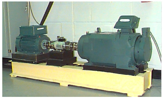
Figure 1.
CWRU bearing test rig.
2.2. Complex Network Model
Complex network makes it possible to undertake a quantitative study on complex systems from different scales and perspectives [23]. This analysis approach abstracts entities in a system into nodes and correlations between entities into edges. A complex network with N nodes can be expressed as . Here represents the set of nodes; , the set of edges; , the number of nodes; and , the number of edges.
At the macro scale, complex network offers various topological properties to describe the overall situation of the network. At the meso-scale, complex network draws upon community detection to mine the system’s pattern. At the micro scale, complex network measures nodes’ importance with centrality indicators. In this article, we focus on the nodes’ properties and base our discussion at the micro scale. Classic centrality indicators include degree, closeness, betweenness and PageRank centrality [24,25,26,27]. The indicators are defined as follows:
(1) Degree centrality (DC) describes the number of other nodes linked to a specific node in the network. DC is expressed as in Formula (1) where . Here, represents the element in row i and column j of the adjacency matrix A; n, the number of nodes in the network; and n − 1, nodes’ maximum degree. In the complex network, a node’s degree centrality shows its range of influence. The higher the degree is, the more important the node is. The average of all nodes’ degree centrality is the average degree.
(2) Closeness Centrality (CC) rules out the interference of special values by calculating the average distance from a specific node to all other nodes in the network. CC is expressed as in Formula (2) where is the average minimum distance from a random node i to other nodes in the network. The shorter the average minimum distance is, the higher the CC is.
(3) Betweenness centrality (BC) shows nodes’ function as bridges and is expressed as in Formula (3). means the number of the shortest paths between nodes s and t, and represents the number of the shortest paths which are between nodes s and t and pass through node i. Node i acting as a bridge reflects i’s control over the transmission of information between other nodes along the shortest paths.
(4) PageRank centrality (PC) shows the quality of a node’s neighbors and is expressed as in Formula (4). is the out-degree of node j. The higher a node’s PC, the more nodes pointing towards it. The specific node also has high-degree friends.
2.3. Incremental Association Markov Blanket (IAMB)
Markov blanket (MB) takes its origin from causal Bayesian network [27]. In its form, Markov blanket of a target variable T is a set of causal features, which makes all other variables probabilistically independent of the target variable T. Markov blanket is defined as in Definition 1.
Definition 1.
Assume that the set of all variables in the domain as U. When the feature subset satisfy the following equations, is defined as the Markov blanket of the target variable T.
Here, P () shows the corresponding probabilities.
Markov blanket discovery is an algorithm to find the Markov blanket (casual feature) of a target variable [28]. The core of this algorithm is learning the Markov boundary of the target variable to find key features through conditional independence tests and identify the causal features in the feature set. To more effectively identify features’ , IAMB is drawn upon in our research [29].
The algorithm adopts a two-stage framework of growth and shrinkage. In the growth stage, candidate variables are sorted through a “dynamic” heuristic process, which helps to overcome the algorithm’s data dependence. IAMB examines causal relationships among features in mainly two stages. First, in the growth stage, through independence tests, variables calculated as related to the target variable T are included in the Markov blanket set. Second, in the shrinkage stage, variables in the MB set calculated as independent of the target variable T are searched for and then deleted. When the MB set stops changing, the search ends. The Markov blanket of target variable T—that is, the causal feature set of the target variable—is obtained.
3. The Feature Selection Approach of Composite Faults
We propose to use casual feature network to select composite fault features. The approach is based on causal relationships and the complex network and includes four steps of data pretreatment, feature extraction, network construction and feature selection. The whole process is shown as in Figure 2.
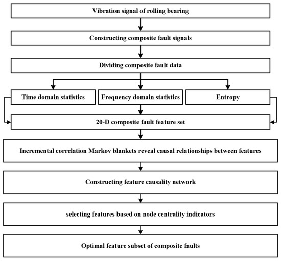
Figure 2.
The process of selecting composite fault features based on the causal feature network.
3.1. Data Pretreatment
We draw upon a linear transient model to mix single faults and construct, thus, the composite fault dataset [21]. The process is as follows:
We first extract nine single fault samples of different types and diameters at the sampling frequency of 12 kHz from the CWRU bearing dataset. The faults are inner race, outer race and rolling element faults and are 0.1778 mm, 0.3556 mm and 0.5334 mm in diameter. Then, we mix the above nine single faults in pairs to obtain 27 types of composite fault signals. Finally, through data pruning, we unify the data format and expand the dataset. Specifically, we intercept the first 102,400 points of each type of composite faults to ensure that the number of sampling points are consistent for each of the vibration data. We divide the 102,400 points of each type of composite faults into 100 segments to ensure that every 1024 points serve as a sample. As the signals generated by the rotation of rolling bearings are periodic, composite fault signals would recur with no qualitative changes in the short period. While ensuring that each signal contains a complete cycle of fault signals, segmenting vibration signals would lead to richer data. The CWRU bearing dataset is sampled at the bearing speed of 1730 rpm—that is, about 28.8 revolutions per second—and at the frequency of 12 kHz. At such a frequency, 12,000 sampling points can be collected every second, and every 417 sampling points show that the bearing completes one revolution. Taking 1024 points as a sample ensures that each piece of data contains a complete rotation cycle with the same starting point. Thus, 27 types of composite faults can generate a set of 2700 samples.
As we only cover fault types in our discussion of composite fault diagnosis here, we relabel the 27 types of composite faults as three types: inner race-outer race, inter race-rolling element and outer race-rolling element.
3.2. Extraction of Composite Fault Features
Feature extraction is a critical link in fault diagnosis. Through transformation, low-dimensional feature space is used to express the original high-dimensional feature space. In this case, the most representative and effective features are obtained. When constructing composite fault feature vectors, to achieve more comprehensive information for the extracted composite fault features, we extract 20 statistical features from three perspectives of time domain statistics, frequency domain statistics and entropy value. The calculation formulas and meanings are depicted in Table A1, Table A2, Table A3 and Table A4 of Appendix A.
Time domain statistics are the statistical value of vibration signals’ time domain parameters and describe how vibration signals change with time. Such statistics include dimensioned and dimensionless parameters. We choose seven dimensioned parameters, including the peak value, peak-to-peak value, average amplitude, root mean square, square root amplitude, variance and standard deviation and record them as fea1–7, respectively. We also select six dimensionless parameters of crest factor, impulse factor, margin factor, shape factor, kurtosis factor and skewness and record them as fea8–13, respectively [30,31].
Frequency domain statistics are the statistical value obtained by performing various operations on signals within the frequency domain after the Fourier transform. Such statistics show the changes in the frequency components of vibration signals. When rolling bearings fail, the frequency components of collected vibration signals change accordingly. Therefore, to obtain features in the frequency domain representative of the faults, we choose five frequency domain statistics of centroid frequency, mean square frequency, root mean square frequency, frequency variance and frequency standard deviation and record them as fea14–18, respectively [32].
Entropy is an indicator to measure the complexity of time series. For rolling bearings, when an unknown fault occurs, the periodic shock signal would lead to an increase in the ordered component of the vibration signal, resulting in a corresponding change in the entropy value. We choose two entropy indicators of power spectral entropy and singular spectral entropy and record them as fea19 and fea20 [33].
3.3. Construction of Causal Feature Network of Composite Faults
The expressions of statistical features have similar calculation methods and may call each other, which leads to redundancies in the feature set. Redundant features will expand the scale of the diagnostic model and slow down the diagnosis. Therefore, feature selection is critical. We have constructed the causal feature network (CFN), introducing the complex network to determine features of relative importance to fault diagnosis results.
The primary task for constructing the composite fault CFN is to define the network’s nodes and edges. As shown in Figure 3, we abstract each feature of composite fault vibration signals as nodes and the causal relationship between features as edges. The CFN of composite faults can be expressed with an adjacency matrix. is to show whether causality exists between features. If causality exists between feature i and j, then ; if no causal relationship exists, then .
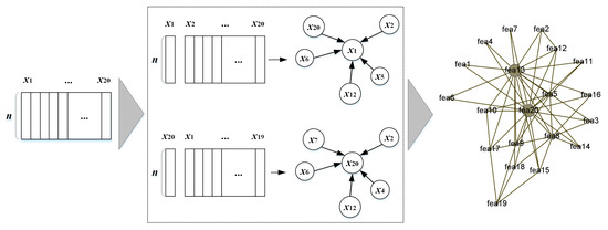
Figure 3.
The process of constructing composite fault CFN.
In defining edges, we use IAMB discovery algorithm to determine the causality between features, as shown in Figure 3. We sequentially take features of the composite fault feature set as the target variables and search for the Markov blanket of the target variables in the remaining 19-dimensional features. Then, we obtain the features that share causal relationships with the target variable features. In this case, we add edges between the target variable features and the features in its Markov blanket set.
3.4. Selection of Important Composite Fault Features
Fault feature selection is to determine the relative importance of features in affecting the fault diagnosis results. When the feature set and its internal causal relationships are abstracted into a network, fault feature selection becomes an issue of nodes’ centrality. Features contribute differently to the representation of composite fault information and the diagnosis results. Quantifying the importance of features in composite fault diagnosis is essential to the feature selection of composite faults. In the complex network, nodes with high centrality play a critical role.
In this section, we propose to use nodes’ centrality indicators to quantify the importance of composite fault features. Specifically, N top-ranked important features are selected in order of node importance (according to one of the centrality indicators), at first. Then, the diagnostic accuracy is obtained by calculating the proportion of sample faults correctly diagnosed in different cases (each centrality index of different numbers of features). The results are finally getting the number of features corresponding to the time when the accuracy reaches the peak.
Taking the DC index as an example, the algorithm first calculates the DC value of each node in the CFN network through Equation (1). Secondly, the 20-dimensional features within the feature set are ranked in ascending order according to the DC value. Thirdly, one feature representative sample with the top ranking is selected to perform the composite fault type recognition task to get the classification accuracy. Then, continue to increase the number of features until we get the accuracy of all the feature representative samples when performing the composite fault type recognition task. Finally, comparing all the accuracy results, the number of features corresponding to the largest accuracy value is the number of features included in the feature set selected according to the DC index.
In the causal feature network, the centrality indicators show the features’ importance in the network. Specifically, degree centrality shows the number of causal relationships of a feature, which indicates the feature’s range of influence. Closeness centrality represents the average minimum distance from a feature to all other features, thus eliminating the interference of special relationships. Betweenness centrality describes a node’s function as a bridge by representing the shortest transmission path through the specific feature and between two other random features. PageRank centrality shows a feature’s position in the network while considering the position of other features which have causal relationships with the specific feature.
4. Results
In this section, we describe the experiments to verify our proposed approach. First, we verify the two correlations between data. Then, we analyze the structural features of the composite fault CFN network. At last, we verify the effectiveness of our feature selection approach.
4.1. Analysis of the Correlations between Features
Detecting causality is the key step to construct the causal feature network. As causal relationships only exist based on correlations, the existence of correlations is the pre-requisite for the study of causal relationships. Therefore, in this section, we base our analysis on both correlations and causal relationships.
We first draw upon Pearson product-moment correlation coefficients (PCCs) to verify the correlations between composite fault features [34]. We undertake correlation analysis and hypothesis testing on the statistical features of 20 signals in the feature set and obtain the correlation coefficient r and its p value among statistical features. Experimental results are as shown in Figure 4. At the assumed significance of α = 0.05, features are mostly correlated with the exception of few features. Especially, strong linear correlations exist among fea1–7 and fea8–12. Therefore, correlations exist and thus can serve as the foundation for our exploration of causal relationships in the composite fault feature set.
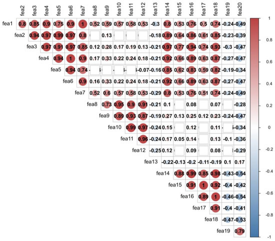
Figure 4.
Heat map of correlations among composite fault features. The output ranges from −1 to +1. Blanks represent no correlation; negative values, negative correlation; and positive values, positive correlation.
Through IAMB algorithm, we further calculate the Markov blanket of every feature, obtaining the subset of features sharing causal relationships with the features in the original feature set. In this case, we get the causality between two random features, and the results are shown in Figure 5. The results show that the feature set has much fewer causal relationships than correlations, and a large amount of correlations are false due to data co-existence. Such false correlations will result in feature redundancies and confuse the interpretation of composite fault diagnosis. Therefore, incorporating causality into the selection of composite fault features can effectively control the size of the optimal feature subset.
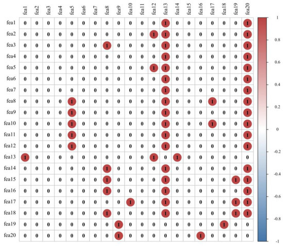
Figure 5.
Visualization of the adjacency matrix of feature causality. The output values are 0 and 1, where 1 represents causal relationships, and 0 represents no such relationships.
4.2. Structural Characteristics of the Causal Feature Network
4.2.1. Macro Characteristics
To grasp the overall situation of the causal feature network of composite faults, we take the macro perspective to analyze the network’s basic characteristics, including the network’s average degree, the network diameter, graph density, average clustering coefficient and average path length. The statistical results are as in Table 1. The results show that the causal feature network is a “small world” network [35]. “Small world”, one example of which is the six degrees of separation theory, reveals a phenomenon in the information society. Although the social network seems huge and complex, nodes in the network are near each other and closely linked. For the causal feature network of composite faults, the average clustering coefficient is high while the average path length is low, which means that the causal feature network shows “small world” effect. And the average path length of 1.78 means that it only takes 1.78 features to achieve causality between any two features in the network.

Table 1.
Descriptive statistics of the network’s basic characteristics.
4.2.2. Nodes’ Centrality of the Causal Feature Network
We use centrality indicators to describe the micro situation of the network and calculate the degree, closeness, betweenness and PageRank centrality of CFN’s nodes. The results, as in Table 2, show that the degree centrality ranges from 0.105 to 0.895; closeness centrality, from 0.514 to 0.905; betweenness centrality, from 0.059 to 59.730; and PageRank centrality, from 0.023 to 0.157.
Table 2.
Table of nodes’ centrality.
Among all features, fea13 and fea20 have the highest degree, closeness, betweenness and PageRank centrality, which shows that these two features share the most and closest causality with other features, and they, as the bridge, are most passed through by the shortest paths between random features. Other nodes, such as fea1, fea4, fea6 and fea7, rank lower in all centrality indicators. The lower ranking of the nodes in degree, closeness and PageRank centrality shows that they share the least and least close causality with other features, and the lower ranking in betweenness centrality shows that they are marginal in the CFN network and serve less as the bridge.
Previous studies selected features based on the feature correlations and fault types. Incorporating centrality indicators, we find that features with high centrality indicators are weakly correlated with fault types. The finding shows that high-centrality features will spread their influence among other nodes through the transmission of causality. Therefore, low-centrality features play a critical role in fault type recognition. As low-centrality features are marginal, causalities related to them are easily neglected. However, such causalities are unique. In this case, we establish the feature selection criteria where we select features in ascending order of nodes’ centrality. We further verify the criteria’s effectiveness.
4.3. Effectiveness of Our Criteria
The core task of feature selection is to obtain the optimal feature subset which requires minimum features to accurately identify fault types. In this section, we use the accuracy of fault diagnosis as the benchmark to verify the effectiveness of our feature selection criteria. We rely on the deep neural network (DNN) for composite fault diagnosis [36]. Specifically, we divide the set of extracted features in an 8:2 ratio. We randomly choose 80% of the set to train the DNN model and use the remaining 20% to test the result of the model. Then, we construct a DNN model for composite fault diagnosis. The model consists of four layers, namely an input layer, two hidden layers and an output layer.
For easier comparison, we set consistent parameters for our following studies. The number of the input layer’s neurons is the same as that of the features in the feature set after selection. The number of neurons in the first hidden layer is set at 500, and that of the second hidden layer is set at 1000. The two layers are both activated with the ReLU function. The number of neurons in the output layer is consistent with the number of type labels, both at 3. The output layer is activated with the sigmoid function. The learning rate of the DNN model is set at 1 × 10⁻⁵. The model is trained with the binary cross-entropy loss function and the Adam optimizer. The training is set for 500 times, and the batch size is set at 16. To counter random and contingent results, we repeat the experiment for 10 times to obtain the average.
4.3.1. Effective Analysis Based on the Fault Diagnosis Results
We verify the effectiveness of feature selection based on the accuracy of composite fault diagnosis. We discuss the accuracy for single features and the feature subset. In the verification, we formulate the criteria for deciding the selection threshold. We also analyze the results of different feature selection approaches.
The effectiveness for single features is the basis for determining the quality of the feature set. We have evaluated the effectiveness for each feature in the feature set and obtained the accuracy of solely relying on any single feature to diagnose composite faults. As shown in Table 3, the accuracy for single features is all above 50%, better than the random probability results. This shows that every feature can be used for composite fault diagnosis, but the resulting accuracy does not satisfy the requirements in real application. We base our further study on the results in Table 3 and build the original feature set (including 20 features) and propose an approach which obtains high accuracy with fewer features.
Table 3.
Accuracy of composite fault diagnosis for single features.
To obtain maximum accuracy with minimum features, we have designed the criteria for threshold selection. Specifically, we rank the centrality indicators of features in the CFN network and increase the number of input features in the DNN according to the ranking. Then we obtain the accuracy of composite fault diagnosis with different numbers of features. We will base our analysis on the accuracy of composite fault diagnosis and the accuracy gain.
Figure 6a shows how the accuracy changes with the size of the feature subset. The accuracy first rises and then drops. The maximum accuracy for different centralities corresponds to different sizes of the optimal subset (referred to here as the optimal number of features). Specifically, for degree and betweenness centrality, the optimal number of features is 10; and for closeness and PageRank centrality, that number is 9. When the optimal number of features is reached, the accuracy will either remain or decrease.
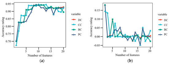
Figure 6.
Diagnosis results using different numbers of features. (a) shows how the accuracy of fault diagnosis changes with different numbers of features. Here, the abscissa is the number of selected features and the ordinate is the accuracy of composite fault diagnosis. (b) shows how the accuracy gain changes with different numbers of features. Here, the abscissa represents i + 1 features, and the ordinate represents the accuracy difference between diagnoses with i and i + 1 features.
Meanwhile, Figure 6b shows how the accuracy gain changes with the size of the feature subset. Overall, the accuracy gain first shrinks and then expands amongst volatilities, and the volatilities eventually become minor. When the number of features reach a certain threshold, more features do not improve the diagnosis and may even hamper the diagnosis. All this verifies that feature selection is necessary as more features do not always improve the results. The model with an appropriate number of features is better than the one with all features in fault diagnosis.
To verify the superiority of the proposed method, we contrast the performance of different selection approaches from the two viewpoints below. In practice, we use the feature subset obtained by different selection approaches as the input for the DNN and get the accuracy of composite fault as the foundation for comparison. Results are shown in Table 4. On the one hand, we contrast the accuracy of the optimal feature subset by using different centrality indicators of the CFN network. We find that the accuracy of our methods is over 94% for composite fault diagnosis, which is a 4% improvement over the results without feature selections. On the other hand, a number of various classical feature selection methodologies are contrasted, including IAMB, RF, SelectKBest. The results illustrate that those accuracies are lower than our approach (that is, 91.62%, 91.78% and 93.34%). Additionally, we screen the features using the feature sensitivity index [37,38]. Because all features have sensitivity values larger than 1, the results demonstrate that this indicator is not instructional for the research topic of this work.
Table 4.
Results of composite fault analysis using different approaches.
In addition, we use the Venn diagram to show the intersection of feature subsets under different approaches. The results are as shown in Figure 7. We find that the feature subsets selected with different centrality indicators have substantial overlaps in certain features. Nine features are chosen when different centrality indicators are used. Meanwhile, the feature subset selected directly with IAMB contains the five remaining features. The results show that the five features are redundant in the feature set and thus counterproductive in composite fault diagnosis.
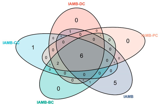
Figure 7.
Venn diagram of features under different selection approaches.
4.3.2. Effective Analysis Based on Randomized Analysis
We undertake random experiments to verify the effectiveness of our selected feature subset. We repeat the experiment for 4000 times under the same conditions and obtain the accuracy distribution of composite fault analysis. We choose 10 random features out of the 20-dimensional feature set to construct the new feature subset to represent samples. We use the new subset as DNN’s input for composite fault diagnosis and then observe the accuracy distribution. The results of randomized experiments are as shown in Figure 8. The accuracies of the random feature subset concentrate around 90%. Under our approach, the accuracy can reach 94.6%. In this case, our approach has an obvious strength in the feature selection of composite fault diagnosis.
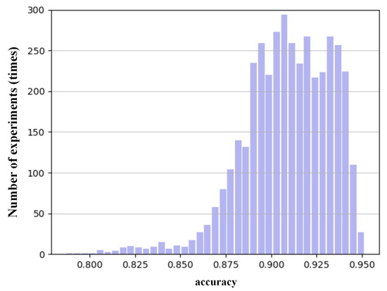
Figure 8.
Accuracy distribution of 4000 random experiments.
5. Conclusions
We focus on how to select effective features out of those extracted from composite fault signals of rolling bearings, thus making the composite fault diagnosis more accurate. We propose a feature selection approach based on the causal feature network (CFN), introducing causality into composite fault diagnosis and expressing such causality with the complex network model. With the model, we take an overall perspective in considering the features and their correlations in the rolling bearing system. Meanwhile, we use causality to express the hidden pattern of interactions within the system. First, we draw upon IAMB discovery algorithm to obtain the causal relationships between composite fault features and construct the complex network to express the causality. Then, we introduce nodes’ centrality indicators to quantify the importance of composite fault features and propose new criteria of threshold selection to determine the number of selected features. At last, we undertake experiments to verify the effectiveness of our approach. Experimental results show that our feature selection approach based on causality and complex network achieves high accuracy. Comparative experiments show that our approach achieves higher accuracy with fewer features.
The following are this paper’s primary conclusions: (1) When a composite fault is diagnosed using a DNN model, the diagnostic accuracy rate often increases before declining as the number of features increases. The growth in the number of characteristics after the accuracy rate reaches its maximum causes the accuracy rate to appear to remain the same or even decline. (2) The accuracy rate is unquestionably increased at first when features are added, but as time goes on, the improvement weakens; after a certain point, adding more features has no further impact on the effectiveness of the diagnosis. (3) Our suggested feature selection approach may surpass the diagnostic effect of 20 features with just about 10 features and achieve higher accuracy with less feature information. (4) Under identical circumstances, the diagnostic accuracy of 4000 randomized trials is concentrated around 90%, whereas the accuracy of our suggested technique can reach 94.6%. Our proposed method has clear advantages for feature selection for compound defect diagnosis.
In this study, we take a comprehensive approach to represent the hidden interaction patterns of rolling bearing systems. Then, causality is used to define the edges of complex networks. Results illustrate that our methods have clear advantages for feature selection for compound defect diagnosis. Future studies could concentrate on two aspects. On one hand, the strength of the causal relationships embedded in the network model allows further comparison of fault diagnosis results. On the other hand, the new index of node centrality should be developed to measure the important features of composite faults.
Author Contributions
Conceptualization, C.Y. and K.G.; methodology, Z.W. and K.G.; investigation, K.G.; data curation, K.G.; writing—original draft preparation, K.G.; writing—review and editing, M.L., Z.W., S.L. and C.Y.; supervision, C.Y. and Z.W. All authors have read and agreed to the published version of the manuscript.
Funding
The work is supported by the National Natural Science Foundation of China (61833002).
Institutional Review Board Statement
Not applicable.
Informed Consent Statement
Not applicable.
Data Availability Statement
The data are available upon request.
Conflicts of Interest
The authors declare no conflict of interest.
Appendix A
Table A1, Table A2, Table A3 and Table A4 present the formulae and meanings of the dimensioned time domain features, dimensionless time domain features, frequency domain features and entropy features.
Table A1.
Time domain features of dimensioned.
Table A1.
Time domain features of dimensioned.
| Feature Nodes | Feature Name | Formula | Significance |
|---|---|---|---|
| Root mean square value | Characterizes the energy of the vibration signal and is sensitive to changes in amplitude | ||
| Peak-to-peak | Describes how violently vibrating a vibration signal | ||
| Peak | Describes the point in the vibration signal where the vibration is most vibrating | ||
| Average amplitude | Describes the overall intensity trend of the vibration signal | ||
| Variance | Characterizes the dynamic component of the signal energy and describes the degree of fluctuation of the vibration signal | ||
| Standard deviation | Describes the degree of fluctuation of the vibration signal | ||
| Square root magnitude | Describes the energy of the vibration signal and is sensitive to changes in amplitude |
Table A2.
Time domain features of dimensionless.
Table A2.
Time domain features of dimensionless.
| Feature Nodes | Feature Name | Formula | Significance |
|---|---|---|---|
| Skewness | Characterize the symmetry of the signal distribution | ||
| Crest factor | Describe the degree of extreme peak value in the waveform, with or without shock | ||
| Waveform factor | Describes changes in the waveform of a vibration signal | ||
| Impulse factor | Describes whether there are abnormal pulses in the signal | ||
| Margin factor | Describes the wear condition of mechanical equipment | ||
| Kurtosis factor | Characterizes the flatness of the vibration signal waveform |
Table A3.
Frequency domain features.
Table A3.
Frequency domain features.
| Feature Nodes | Feature Name | Formula | Significance |
|---|---|---|---|
| Centroid frequency | Describes the location of the center of the vibration signal in the frequency domain | ||
| Mean square frequency | Describes the location distribution of the vibration signal in the frequency domain in the main frequency band | ||
| Root mean square frequency | Describes the radius of inertia of the vibration signal centered at the center of gravity frequency | ||
| Frequency variance | Describes the frequency distribution of the vibration signal in the frequency domain | ||
| Frequency standard deviation | Characterizes the overall off-center fluctuation of the vibration signal in the overall frequency domain |
Table A4.
Entropy.
Table A4.
Entropy.
| Feature Nodes | Feature Name | Formula | Significance |
|---|---|---|---|
| Power spectral entropy | Describes the complexity of the signal’s energy distribution in the frequency domain | ||
| Singular spectral entropy | Describes the complex state of a time series signal |
References
- Yu, J.; Hua, Z.; Li, Z. A new compound faults detection method for rolling bearings based on empirical wavelet transform and chaotic oscillator. Chaos Solitons Fractals 2016, 89, 8–19. [Google Scholar] [CrossRef]
- Pang, B.; Nazari, M.; Tang, G. Recursive variational mode extraction and its application in rolling bearing fault diagnosis. Mech. Syst. Signal Process. 2022, 165, 108321. [Google Scholar] [CrossRef]
- Glennan, S. Mechanisms and the nature of causation. Erkenntnis 1996, 44, 49–71. [Google Scholar] [CrossRef]
- Dhamande, L.; Chaudhari, M. Compound Gear-Bearing Fault Feature Extraction Using Statistical Features Based on Time-Frequency Method. Measurement 2018, 125, 63–77. [Google Scholar] [CrossRef]
- Zheng, J.; Pan, H.; Tong, J.; Liu, Q. Generalized refined composite multiscale fuzzy entropy and multi-cluster feature selection based intelligent fault diagnosis of rolling bearing. ISA Trans. 2022, 123, 136–151. [Google Scholar] [CrossRef]
- Li, J.; Cheng, K.; Wang, S.; Fred, M.; Robert, P.; Tang, J.; Liu, H. Feature Selection: A Data Perspective. ACM Comput. Surv. 2017, 50, 6. [Google Scholar] [CrossRef]
- Drotár, P.; Gazda, J.; Smékal, Z. An experimental comparison of feature selection methods on two-class biomedical datasets. Comput. Biol. Med. 2015, 66, 1–10. [Google Scholar] [CrossRef]
- Zhang, B.; Zhang, Y.; Jiang, X. Feature selection for global tropospheric ozone prediction based on the BO-XGBoost-RFE algorithm. Sci. Rep. 2022, 12, 9244. [Google Scholar] [CrossRef]
- Sun, L.; Wang, T.; Ding, W.; Xu, J.; Lin, Y. Feature Selection Using Fisher Score and Multilabel Neighborhood Rough Sets for Multilabel Classification. Inf. Sci. 2021, 578, 887–912. [Google Scholar] [CrossRef]
- Barile, C.; Casavola, C.; Pappalettera, G.; Kannan, V. Laplacian score and K-means data clustering for damage characterization of adhesively bonded CFRP composites by means of acoustic emission technique. Appl. Acoust. 2022, 185, 108425. [Google Scholar] [CrossRef]
- Liu, H.; Zhou, M.; Liu, Q. An embedded feature selection method for imbalanced data classification. IEEE/CAA J. Autom. Sin. 2019, 6, 703–715. [Google Scholar] [CrossRef]
- Sun, L.; Zhang, J.; Ding, W.; Xu, J. Mixed measure-based feature selection using the Fisher score and neighborhood rough sets. Appl. Intell. 2022, 52, 17264–17288. [Google Scholar] [CrossRef]
- Bouke, M.; Abdullah, A.; ALshatebi, S.; Mohd, T.; Hayate, E. An intelligent DDoS attack detection tree-based model using Gini index feature selection method. Microprocess. Microsyst. 2023, 98, 104823. [Google Scholar] [CrossRef]
- Wang, N.; Li, Q.; Du, X.; Zhang, Y.; Zhao, L.; Wang, H. Identification of main crops based on the univariate feature selection in Subei. J. Remote Sens. 2017, 21, 519–530. [Google Scholar] [CrossRef]
- Lee, J.; Jeong, J.-Y.; Jun, C.-H. Markov blanket-based universal feature selection for classification and regression of mixed-type data. Expert Syst. Appl. 2020, 158, 113398. [Google Scholar] [CrossRef]
- Guo, X.; Yu, K.; Cao, F.; Li, P.; Wang, H. Error-aware Markov blanket learning for causal feature selection. Inf. Sci. 2022, 589, 849–877. [Google Scholar] [CrossRef]
- Tran, M.; Elsisi, M.; Liu, M. Effective feature selection with fuzzy entropy and similarity classifier for chatter vibration diagnosis. Measurement 2021, 184, 109962. [Google Scholar] [CrossRef]
- Yong, Z.; Donner, R.; Marwan, N.; Donges, J.; Kurths, J. Complex network approaches to nonlinear time series analysis. Phys. Rep. 2019, 787, 1–97. [Google Scholar] [CrossRef]
- Ji, Z.; Fu, Z.; Zhang, S. Fault diagnosis of diesel generator set based on optimized NRS and complex network. J. Vib. Shock. 2020, 39, 246–251. [Google Scholar] [CrossRef]
- Chen, A.; Mo, Z.; Jiang, L.; Pan, Y. A complex network association clustering-based diagnosis method for the separation of composite fault features. Vib. Shock. 2016, 35, 76–81. [Google Scholar] [CrossRef]
- Lu, J.; Cheng, W.; He, D.; Zi, Y. A novel underdetermined blind source separation method with noise and unknown source number. J. Sound Vib. 2019, 457, 67–91. [Google Scholar] [CrossRef]
- Smith, W.; Randall, R. Rolling Element Bearing Diagnostics Using the Case Western Reserve University Data: A Benchmark Study. Mech. Syst. Signal Process. 2015, 64, 100–131. [Google Scholar] [CrossRef]
- Lambiotte, R.; Rosvall, M.; Scholtes, I. From networks to optimal higher-order models of complex systems. Nat. Phys. 2019, 15, 313–320. [Google Scholar] [CrossRef] [PubMed]
- Zhong, S.; Zhang, H.; Deng, Y. Identification of influential nodes in complex networks: A local degree dimension approach. Inf. Sci. 2022, 610, 994–1009. [Google Scholar] [CrossRef]
- Kopsidas, A.; Kepaptsoglou, K. Identification of critical stations in a Metro System: A substitute complex network analysis. Phys. A Stat. Mech. Its Appl. 2022, 596, 127123. [Google Scholar] [CrossRef]
- Zhang, M.; Huang, T.; Guo, Z.; He, Z. Complex-network-based traffic network analysis and dynamics: A comprehensive review. Phys. A Stat. Mech. Its Appl. 2022, 607, 128063. [Google Scholar] [CrossRef]
- Wu, X.; Jiang, B.; Lv, S.; Wang, X.; Chen, H. Review of causal feature selection algorithms based on Markov boundary discovery. Pattem Recognit. Aitificial Intell. 2022, 35, 422–438. [Google Scholar] [CrossRef]
- Tian, G.; Qiang, J. Efficient Markov Blanket Discovery and Its Application. IEEE Trans. Cybern. 2016, 47, 1–11. [Google Scholar] [CrossRef]
- Wan, P.; Wu, C.; Lin, Y.; Ma, X. Driving anger states detection based on incremental association markov blanket and least square support vector machine. Discret. Dyn. Nat. Soc. 2019, 2019, 1–17. [Google Scholar] [CrossRef]
- Prieto, M.; Cirrincione, G.; Espinosa, A.; Ortega, J.; Henao, H. Bearing Fault Detection by a Novel Condition-Monitoring Scheme Based on Statistical-Time Features and Neural Networks. IEEE Trans. Ind. Electron. 2013, 60, 3398–3407. [Google Scholar] [CrossRef]
- Rauber, T.W.; de Assis Boldt, F.; Varejao, F.M. Heterogeneous Feature Models and Feature Selection Applied to Bearing Fault Diagnosis. IEEE Trans. Ind. Electron. 2015, 62, 637–646. [Google Scholar] [CrossRef]
- He, Z.; Shi, T.; Xuan, J. Milling tool wear prediction using multi-sensor feature fusion based on stacked sparse autoencoders. Measurement 2022, 190, 1–10. [Google Scholar] [CrossRef]
- Wei, J.; Yu, L.; Zhu, L.; Zhou, X. RF fingerprint extraction method based on Ceemdan and multidomain joint entropy. Wirel. Commun. Mob. Comput. 2022, 2022, 5428280. [Google Scholar] [CrossRef]
- Zhang, M.; Li, W.; Zhang, L.; Jin, H.; Mu, Y.; Wang, L. A Pearson correlation-based adaptive variable grouping method for large-scale multi-objective optimization. Inf. Sci. 2023, 639, 118737. [Google Scholar] [CrossRef]
- Kuperman, M.; Abramson, G. Small world effect in an epidemiological model. Phys. Rev. Lett. 2001, 86, 2909. [Google Scholar] [CrossRef] [PubMed]
- LeCun, Y.; Bengio, Y.; Hinton, G. Deep learning. Nature 2015, 521, 436–444. [Google Scholar] [CrossRef]
- Guo, X.; Wu, N.; Cao, X. Fault diagnosis of rolling bearing of mine ventilator based on characteristic fusion and DBN. Ind. Mine Autom. 2021, 47, 14–20. [Google Scholar] [CrossRef]
- Kuang, T.; Li, Z.; Zhu, W.; Xie, J.; Ju, J.; Liu, J.; Xu, J. The impact of key strata movement on ground pressure behavior in the Datong coalfield. Int. J. Rock Mech. Min. Sci. 2019, 119, 193–204. [Google Scholar] [CrossRef]
Disclaimer/Publisher’s Note: The statements, opinions and data contained in all publications are solely those of the individual author(s) and contributor(s) and not of MDPI and/or the editor(s). MDPI and/or the editor(s) disclaim responsibility for any injury to people or property resulting from any ideas, methods, instructions or products referred to in the content. |
© 2023 by the authors. Licensee MDPI, Basel, Switzerland. This article is an open access article distributed under the terms and conditions of the Creative Commons Attribution (CC BY) license (https://creativecommons.org/licenses/by/4.0/).