Sentinel-2 Observation of Water Color Variations in Inland Water across Guangzhou and Shenzhen after the Establishment of the Guangdong-Hong Kong-Macao Bay Area

Abstract

Guangzhou and Shenzhen are two core cities in the Guangdong-Hong Kong-Macao Greater Bay Area (GBA). It is increasingly important to regulate water quality in urban development. The Forel–Ule Index (FUI) can be obtained by optical data and is an important indicator. Therefore, we used Sentinel-2 to calculate the FUI of 41 lakes and reservoirs in Guangzhou and Shenzhen from January to December in 2016–2021, and analyzed their spatio-temporal variations, including spatial distributions, seasonal variations, and inter-annual variations. We also performed a correlation analysis of driving factors. In Guangzhou, the FUI was low in the north and west, and high in the south and east. In Shenzhen, the FUI was high in the west and low in the east. Moreover, 68% of the lakes and reservoirs in Guangzhou exhibited seasonal variations, with a low FUI in summer and autumn, and high levels in spring and winter. Shenzhen had the lowest FUI in autumn. Furthermore, 36% of the lakes and reservoirs in Guangzhou exhibited increasing inter-annual variations, whereas Shenzhen exhibited stable and decreasing inter-annual variations. Among the 41 lakes and reservoirs analyzed herein, the FUI of 10 water areas were positively correlated with precipitation, while the FUI of 31 water areas were negatively correlated with precipitation. Increased precipitation leads to an increase in external pollutants and sediment, as well as the resuspension of substances in the water, resulting in more turbid water. Therefore, an increase in precipitation is positively correlated with the FUI, whereas a decrease in precipitation is negatively correlated with the FUI. These findings can be used to design suitable management policies to maintain and control the local water quality.

1. Introduction

The Pearl River Delta has been developed into the GBA, which is one of the four largest bays in the world, and is the economic center of not only Guangdong province, but also the entire country. Although it is located in the second largest estuary in China, this region faces huge water problems. The GBA is densely populated. Owing to its large-scale industrial and agricultural development and densely distributed cities and towns, water pollution is extremely prominent in the region, which seriously hinders its sustainable development. Surface water environmental quality reports from Guangdong province in the first half of 2018 showed that the surface water quality was poor (accessed on 17 July 2018; http://www.gdep.gov.cn/hjjce/hjxt/201807/t20180717_240642). Guangzhou and Shenzhen are becoming increasingly important in the GBA. Therefore, it is imperative to analyze the surface water quality in Guangzhou and Shenzhen.

Traditional water-quality-monitoring methods collect a set number of sampling points in a specific water area, after which, on-site sampling is conducted. Such methods are not only time-consuming and energy intensive, but also provide limited information with respect to spatio-temporal variations, particularly in inaccessible water areas. Remote sensing technology is advantageous in terms of both a wide monitoring range and a short monitoring cycle [1,2]. In addition, remote sensing can retrieve some traditional parameters, such as water clarity (SDD) [3,4,5], chlorophyll a (Chla) [6,7,8], suspended particulate matter (SPM) concentration [9,10], colored dissolved organic matter (CDOM) [11], etc. However, owing to the complex optical properties of inland water, many algorithms for parameters are limited to different regions and seasons [12,13].

To apply remote sensing to analyze the variations in water quality, it is necessary to select parameters that are invariant by optical properties, such as water color. Water color can provide regional and global water quality characteristics, and is used to monitor lakes and reservoirs. Water color results from the interactions between sunlight and the substances (Chla, SPM, and CDOM), and is related to the absorption and scattering of the substances [14].

Previous studies have applied water color parameter analyses for water quality research. Alfoldi and Munday (1978) used Landsat data for chromaticity analysis and found that it was a rapid and simple water quality monitoring method [15]. Related studies have also shown that differences in the water components produced considerable differences in the main wavelength range of the water color. Related studies have indicated that, owing to the uncertainty of the substances in the water, extensive retrieval methods for water quality parameters using water color analysis and the band ratio method have certain limitations and instabilities [16].

Li et al. (2016) analyzed water quality variations of ten lakes in China by extracting the Forel–Ule Index (FUI) from the Moderate Resolution Imaging Spectrometer (MODIS) [17]. Furthermore, Wang et al. (2018) used MODIS to retrieve the trophic status of water using the FUI, and analyzed the variations in global inland water [18]. The FUI dataset for global lakes and reservoirs from 2000 to 2018 based on MODIS was then released, which provided information on spatio-temporal variations in water color of global lakes and reservoirs during the period [19].

Zhao et al. (2021) [20] applied the SDD model proposed by Wang et al. (2020) [21] to Sentinel-2 to calculate the SDD of the Yangtze River mainstream and analyze its spatio-temporal variations from 2017 to 2020 [20]. Sentinel-2 has been used to analyze the water color variations of Baiyangdian Lake [22]. Furthermore, Sentinel-2 has been used to calculate the water hue angle α and determine the threshold for screening water color anomalies, which achieved good results in Heilongjiang and Hebei province [23].

The Development Plan for the GBA was issued on 18 February 2019, and officially announced the construction of the GBA, in which Guangzhou and Shenzhen are two important cities. Therefore, we analyzed water color variations of 41 inland lakes and reservoirs (larger than 0.5 km²) in Guangzhou and Shenzhen after the construction of the GBA. We used Sentinel-2 to produce monthly, quarterly and annual FUI products, and analyzed their spatial distributions, seasonal and inter-annual variations, and driving factors.

2. Materials and Methods

2.1. Study Area

Guangzhou and Shenzhen, they are located in Guangdong Province (Figure 1). They are increasingly important core cities in the GBA as well. They have no freezing periods throughout the year and are abundant in rainfall, and the rainy season extends from April to September.

There are 41 lakes and reservoirs larger than 0.5 km² in Guangzhou and Shenzhen: 22 in Guangzhou, in the Conghua, Huadu, Luogang, and Zengcheng areas, and 19 in Shenzhen, in the Bao’an, Futian, Longgang, Yantian, and Luohu areas.

2.2. Research Data

(1)

Sentinel-2

Sentinel-2, at an orbital height of 786 km, is equipped with a multi-spectral imager (MSI) with 13 spectral bands, an image width of 290 km, and spatial resolutions of 10, 20, and 60 m. The revisit time of each satellite is 10 d. Sentinel-2A and 2B are complementary; thus, the revisit time is shortened to 5 d. In addition, the revisit time of Sentinel-2 in the mid-latitudes can be shortened to 2–3 d. Sentinel-2 has high temporal and spatial resolutions, a relatively rich spectral band, and a wide imaging width. During 2016–2018, Sentinel-2 only included Level-1C, which must be processed using Sen2Cor to obtain Level-2A surface reflectance (SR). Since 2019, SR can be obtained directly from the official ESA through Sen2Cor. Their spectral response functions are very similar; thus, the two satellites can be regarded as the same (Figure 2).

(2)

Auxiliary data

To better analyze spatio-temporal variations in external factors affecting long-term water quality, we performed this study in Guangzhou (http://swj.gz.gov.cn/) and Shenzhen (http://swj.sz.gov.cn/). Precipitation data for each administrative region from January to December of 2016–2021 were obtained from the Water Affairs Bureau website.

Table 1. Precipitation stations in Guangzhou City and Shenzhen.

Guangzhou City		Shenzhen City
Area	Station	Area	Station
Conghua Area	Taipingpu Station	Baoan Area	Shiyan Station
	Huanglongdai Station		Luotian Station
Huadu Area	Jiuwantan Station		Tiegang Station
		Futian Area	Xili Station
Huangpu Area	Huangpu Station	Longgang Area	Qinglinjing Station
		Dapeng New Area	Nanao Station
Zengcheng Area	Paitan Station	Yantian Area	Sanzhoutian Station
		Luohu Area	Shenzhen Station

presents the precipitation stations in Guangzhou and Shenzhen used in this study. Wind speeds were obtained from the National Centers for Environmental Information (NCEI) of the National Oceanic and Atmospheric Administration (NOAA) (https://www.ncei.noaa.gov/data/global-summary-of-the-day/archive/). Statistics on the residents, tourism, and Gross Domestic Product (GDP) of Guangzhou and Shenzhen were obtained from the official website of the GBA (https://www.dsec.gov.mo/BayArea/zh-MO/#s5).

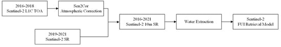
2.3. Image Pre-Processing

Although Sentinel-2 has been widely used, there is no precise atmospheric correction for water. Wang et al. (2016) proposed a secondary simple correction method for SR data, which can remove sun glint and residual noise effects from SR data [24]. The correction formula is:

$$R_{rs}\left(\mathsf{\lambda }\right)=\frac{R_{rs}\left(\mathsf{\lambda }\right)-\min \left(R_{rs}\left(\mathrm{NIR}\right):R_{rs}\left(\mathrm{SWIR}\right)\right)}{\pi }$$

(1)

where min (R_rs(NIR): R_rs(SWIR)) represents the minimum value of both NIR and SWIR bands, and R_rs(λ) represents the raw R_rs of the visible bands R_rs(443), R_rs(490), R_rs(560), and R_rs(705) of Sentinel-2 data.

2.4. Waterbody Extraction Method

This is the most commonly used method to identify water by water index. It is efficient, and easy to apply; however, it cannot effectively restrain interference factors around the water, such as trees, shadows, and asphalt roads. Support Vector Machine (SVM), Decision Tree (DT), and other classification methods are required to manually draw high-precision samples with rich water types in advance; however, the sample selection is very complex and time-consuming, and the sample precision will also affect the water extraction results.

To accurately identify water, we selected a global surface coverage product released by Gong Peng [25] in 2019 as the reference area. Because a waterbody is affected by external factors, the range of the product was expanded by 2 pixels and then used as the buffer for water, while the gray image of the Multi-Band Water Index (MBWI) [26] was used as enter data (MBWI gray image). K-Means was used to identify the waterbody within the buffer. The flowchart is Figure 3.

MBWI = 2 R_rs(Green) − R_rs(Red) − R_rs(NIR) − R_rs(SWIR1) − R_rs(SWIR2)

(2)

The central wavelengths of R_rs(Green), R_rs(Red), R_rs(NIR), R_rs(SWIR1), and R_rs(SWIR2) in Equation (2) are 560 nm, 665 nm, 842 nm, 1610 nm, and 2190 nm.

Determining the optimal threshold using the conventional threshold method is repetitive and tedious, and human error may be introduced into the classification results. The unsupervised classification method has the advantage of low human involvement and efficiency. K-means clustering is an effective unsupervised classification. The water and non-water classification results were obtained by K-means clustering of water body index results. For the K-means clustering parameters, the classification number, change threshold, and maximum iteration numbers were 10, 0.01, and 10,000, respectively. After clustering, we obtained water and non-water classification results [26]. The result of water extraction is Figure 4.

2.5. Calcualtion

The FUI was calculated based on the CIE-XYZ standard color system proposed by the International Commission on Illumination (CIE), in which the X, Y, Z tristimulus values were first proposed. Sentinel-2 has five visible light bands, and the formula for calculating the X, Y, Z tristimulus values is Equation (3) [27]:

$$\left\{\begin{array}{c}X=11.756R\left(443\right)+6.423R\left(490\right)+53.696R\left(560\right)\\ +32.028R\left(665\right)+0.529R\left(705\right)\\ Y=1.744R\left(443\right)+22.289R\left(490\right)+65.702R\left(560\right)\\ +16.808R\left(665\right)+0.192R\left(705\right)\\ Z=62.696R\left(443\right)+31.101R\left(490\right)+1.778R\left(560\right)\\ +0.015R\left(665\right)+0.000R\left(705\right)\end{array}\right.$$

(3)

The Landsat 8 Operational Land Imager (OLI) has four visible light bands, and the formula is Equation (4):

$$\left\{\begin{array}{c}X=11.053R\left(443\right)+6.950R\left(483\right)+51.135R\left(561\right)+34.457R\left(661\right)\\ Y=1.320R\left(443\right)+21.053R\left(483\right)+66.023R\left(561\right)+18.034R\left(661\right)\\ Z=58.038R\left(443\right)+34.931R\left(483\right)+2.606R\left(561\right)+0.016R\left(661\right)\end{array}\right.$$

(4)

The relevant information is in

Table 2. Spectral bands for the Sentinel-2 and Landsat 8 OLI.

Sentinel-2		Landsat 8 OLI
Central Wavelength (nm)	Bands	Central Wavelength (nm)	Bands
443	Coastal Blue	443	Coastal Blue
490	Blue	483	Blue
560	Green	561	Green
665	Red	661	Red
705	Vegetation Red Edge

.

The chromaticity coordinates in the CIE were calculated based on tristimulus values, and the results of the chromaticity coordinates were normalized to 0–1 (Figure 5 and

Table 3. Chromaticity coordinates and hue angles (α) of the FUI [18].

FUI	x	y	$\mathit{\alpha }$ (°)
1	0.191363	0.166919	40.467
2	0.198954	0.199871	45.19626
3	0.210015	0.2399	52.85273
4	0.226522	0.288347	67.16945
5	0.245871	0.335281	91.29804
6	0.266229	0.37617	122.5852
7	0.290789	0.411528	151.4792
8	0.315369	0.440027	170.4629
9	0.336658	0.461684	181.4983
10	0.363277	0.476353	191.8352
11	0.386188	0.486566	199.0383
12	0.402416	0.4811	205.0622
13	0.416243	0.47368	210.5766
14	0.431336	0.465513	216.5569
15	0.445679	0.457605	222.1153
16	0.460605	0.449426	227.6293
17	0.475326	0.440985	232.8302
18	0.488676	0.43285	237.3523
19	0.503316	0.424618	241.7592
20	0.515498	0.416136	245.5513
21	0.528252	0.408319	248.9529

). Therefore, a new coordinate system was obtained [18] that is described by Equation (5):

$$\left\{\begin{array}{c}x=\frac{X}{X+Y+Z}\\ y=\frac{Y}{X+Y+Z}\end{array}\right.$$

(5)

Finally, the hue angle $\alpha$ was obtained [18] by Equation (6):

$$\alpha =arctan\left(\frac{y-y_w}{x-x_w}\right)\times \frac{180}{\pi }+180$$

(6)

where $y_w$ and $x_w$ are $\left(\frac{1}{3},\frac{1}{3}\right)$.

To eliminate hue angle $\alpha$ deviations caused by band dispersion and band setting $\Delta$, we established an error polynomial fitting formula based on the water surface reflectance database and added the system deviation simulated by the polynomial to the hue angle $\alpha$ calculated from the multi-spectral images. The method had the effect of eliminating bias [29].

The optimal linear relationship between the hue angle $\alpha$ calculated from the hyperspectral data and that calculated by the satellite sensor was obtained by finely correcting the hue angle $\alpha$. Specifically, the hue angle $\alpha$ was corrected by compensating for the linear interpolation between the natural water spectrum and the sensor band. Owing to sensor band limitations, a large offset was not generated randomly. The calibration formula of the hue angle $\alpha$ based on the Sentinel-2 data is as follows [20]:

$$\Delta =46.2094a^5-412.256a^4+1385.5708a^3-2128.364a^2+1443.7115a-341.6433$$

(7)

The calibration formula of hue angle $\alpha$ based on the Landsat 8 OLI is as follows [30]:

$$\Delta =-52.819a^5+334.88a^4-758.26a^3+746.324a^2-315.18a+39.761$$

(8)

where a is the hue angle $\alpha$ divided by 100. By correcting the hue angle $\alpha$, its value is closer to the actual water color. In this study, the definition of the hue angle $\alpha$ was based on the point of equal-energy white light, and increased with the main wavelength of color. Note that the definition of the hue angle $\alpha$ in this study is different from that of van der Woerd and Wernand in theirs [29]. Each FUI represents the hue angle $\alpha$ range, with a smaller FUI indicating clearer water, whereas a larger FUI indicates more turbid water.

2.6. Temporal and Spatial Aggregation

Since Guangzhou and Shenzhen do not have a freezing period, FUI was calculated from January to December of 2016–2021. Based on Sentinel-2, the FUI of 41 lakes and reservoirs in Guangzhou and Shenzhen were obtained, as well as their spatial distributions, their seasonal and interannual variations, and the driving factors affecting the variations in the FUI. Because the water is dynamic, calculating the FUI from a single-day image resulted in greater randomness; therefore, we performed our statistical analysis using the monthly average effective FUI to reflect the variations in lake and reservoir water quality more faithfully. The season division is

Table 4. Season division.

Month	Season
March, April, May	Spring
June, July, August	Summer
September, October, November	Autumn
December, January, February	Winter

.

We used remote sensing images with cloud cover ≤30% and no significant cloud cover above the water body as valid data. If multiple effective data were obtained every month, the average of the multi-scene effective data were calculated as the monthly average of the monthly FUI. If only single-scene effective data were available in a given month, the scene image of the FUI represented the average results for the month. Using the statistical monthly average FUI reduced the random error generated by single-scene data. The statistic result of valid Setinel-2 data is Figure 6.

2.7. Evaluation Index

Trend changes analyzed by the Mann–Kendall (M–K) significance test [31,32] in Guangzhou and Shenzhen from 2016 to 2021. The M–K test uses a standardized Z-statistic to determine the monotonic trend of the data, where Z > 0 indicates that the data has an increasing trend and Z < 0 indicates that the data has a decreasing trend (

Table 5. Mann–Kendall significance test.

Z	$\mathit{\alpha }$	Significance
≥2.58	≤0.01	Extremely significant
≥1.96	≤0.05	Significant
<1.96	>0.05	Not significant

Note: $\alpha$ represents the significance level; Z represents the standard confidence value.

).

The coefficient of variation (CV), mean relative error (MRE), and root mean square error (RMSE) were used to calculate the evaluation index. The CV compares the dispersion degrees of different groups of data. Smaller CV values indicate smaller degrees of variation of the data; larger CV values indicate greater degrees of variation. These parameters were calculated as follows:

$$\mathrm{MRE}=\frac{1}{n}\frac{\left|A-A^{\prime }\right|}{A}$$

(9)

$$\mathrm{RMSE}=\sqrt{\frac{{\sum }_1^n{\left(A-A^{\prime }\right)}^2}{n}}$$

(10)

$$\mathrm{CV}=\frac{\mathrm{Standard}\mathrm{deviation}}{\mathrm{Mean}\mathrm{value}}$$

(11)

$$\mathrm{Standard}\mathrm{deviation}=\sqrt{\frac{{\sum }_{i-1}^n{\left(A_i-\overline{A}\right)}^2}{n}}$$

(12)

$$\mathrm{Mean}\mathrm{value}=\frac{A_1+\cdots +A_n}{n}=\frac{{\sum }_{i=1}^n{A}_i}{n}$$

(13)

where A is the result of Landsat 8 OLI, A′ is the result of Sentinel-2, and n is the number of verification points.

The correlation coefficient is used to explain the correlation between two parameters. Positive correlations indicate that when one variable increases/decreases, the other also increases/decreases. The Pearson correlation coefficient (PCC) represented the correlation between two variables, as follows:

$$rho=\frac{cov\left(X,Y\right)}{{\sigma }_X{\sigma }_Y}=\frac{\sum XY-\frac{\sum X\sum Y}{N}}{\sqrt{\left(\sum X^2-\frac{{\left(\sum X\right)}^2}{N}\right)\left(\sum Y^2-\frac{{\left(\sum Y\right)}^2}{N}\right)}}$$

(14)

3. Results

3.1. Accuracy Evaluation of the FUI

Owing to a lack of in situ data from inland water in Guangzhou and Shenzhen, the accuracy evaluation was mainly divided into two parts to show the universality and stability of the FUI in a large-scale study area.

First, the FUI was calculated using Sentinel-2 (23 May 2019) from Baiyangdian Lake, which has complex optical characteristics. Second, the in situ R_rs(λ) acquired from Baiyangdian Lake on 21 and 22 May 2019 was obtained and the results were compared. The accuracy evaluation indices were MRE and RMSE. The MRE and RMSE were 3.54% and 0.57, respectively. Figure 7 shows a scatterplot of the accuracy evaluation of the FUI in Baiyangdian Lake.

Xu et al. [33] applied the FUI to Landsat 8 OLI data and found that the FUI has good accuracy and universality, and can be applied to large-scale water quality variations. Therefore, the FUI calculated using the Landsat 8 OLI data were used as the actual values to evaluate Sentinel-2 data. Seventy verification points were selected for lakes and reservoirs in Guangzhou and Shenzhen, and Sentinel-2 and Landsat 8 transited this region on 5 December 2021.

If a corresponding number of verification points are selected off the shore, the shore may be affected by optical shallow water or pollutants; However, the spatial resolution is different. If a verification point is located on the edge, it may also be distributed by land proximity effects. Thus, the distance between the verification points and the edge was set as larger than 5 pixels, allowing the selected points to reduce influence factors. Figure 8 shows selected verification points in the study area.

Figure 5 shows that there are 21 FUI levels, each of which represents a discrete hue angle $\alpha$ range. To compare the results of the two sensors more accurately, we utilized the hue angle $\alpha$ instead of the FUI for accuracy evaluation. With each verification point as the center, Sentinel-2 selects a 9 × 9 pixels area and the Landsat 8 OLI selects a 3 × 3 pixels area. The spatial resolutions of the two sensors differ, which can ensure that the selected area of each verification point is consistent. The influence of single-pixel randomness was reduced. The mean value of the CV of 70 verification points in Sentinel-2 and Landsat 8 OLI were 1.1% and 5.8%, respectively. These CV results were similar to those obtained previously, indicating that the results are stable and reliable. The PCC was calculated as 0.77. Therefore, the method was shown to be reliable. Previous studies have cross-verified the water color parameters retrieved by MODIS, Landsat 8 OLI, and Sentinel-2, and have good application potential [20,34,35].

3.2. Spatial Distribution

Figure 9a shows the spatial distribution of 22 lakes and reservoirs in Guangzhou, located in the Conghua, Huadu, Luogang, and Zengcheng areas. Their overall spatial distributions were low in the north and west, and high in the south and east. The FUI ranged from 6.3 to 9.5 in the Conghua area in the north, and ranged from 7.3–9.5 in the Luogang area in the south. Moreover, the FUI ranges of the Huadu area in the west and the Zengcheng area in the east were 7.7–11.2 and 8.0–12.3, respectively. Figure 9b shows the spatial distribution of the FUI of 19 water areas in Shenzhen, located in the Bao’an, Longgang, Futian, Luohu, and Yantian areas. The overall spatial distribution was high in the west and low in the east. The FUI ranges in Bao’an, Longgang, Futian, Luohu, and Yantian areas were 8.2–9.9, 7.3–9.1, 8.4, 8.3, and 6.3, respectively.

3.3. Seasonal Variations

The 41 lakes and reservoirs were numbered, (i.e., GZ1-GZ22 in Guangzhou and SZ1-SZ19 in Shenzhen). According to the statistics of the evaluation standards and trends of 41 lakes and reservoirs in Guangzhou and Shenzhen (Figure 10, Figure 11 and Figure 12), only a few lakes and reservoirs exhibited significant seasonal FUI variations, while most of the lakes and reservoirs exhibited no significant variations. Figure 10 shows the seasonal variations of 22 water areas in Guangzhou, 68% of which had lower FUIs in summer/autumn and higher FUIs in winter/spring, while 32% of the lakes and reservoirs exhibited slightly different variation trends. Among them, the FUI of GZ4 was lower in autumn/winter, and higher in spring/summer, whereas GZ11 exhibited the opposite trend. Furthermore, the FUI of GZ12 was lower in spring/autumn, and higher in summer/winter. The FUIs of GZ14 and GZ18 were the lowest in summer and the highest in winter. The seasonal variations in all lakes and reservoirs were extremely similar, and the FUI was the lowest in autumn.

3.4. Inter-Annual Variations

Among the 19 reservoirs in Shenzhen, the FUI of 9 decreased, while the rest remained relatively stable. As for inland water quality, that of Shenzhen was better than that of Guangzhou. As shown in Figure 13, Figure 14 and Figure 15, in 2016–2021, the annual variations in the FUI of the 41 lakes and reservoirs were not significant, indicating that the water quality did not change significantly and remained at a good level. Figure 14 and Figure 15 show the results of the annual variations in the FUI of 41 lakes and reservoirs in Guangzhou and Shenzhen from 2016 to 2021, respectively. Among the 41 lakes and reservoirs, 36% had increased FUI trends, 30% had decreased FUI trends, and 34% were relatively stable. For 22 lakes in Guangzhou, their FUI trends were relatively stable.

4. Discussion

The water quality variations of inland, coastal, and ocean water are somewhat similar, and all have exhibited decreasing trends [36]. In different regions, the factors leading to variations in water quality differ [18,37,38,39]. The FUI variations of lakes and reservoirs in Guangzhou and Shenzhen were found to be mainly caused by natural and human factors.

4.1. Meteorological Factors

The natural factors that affected the variations in water quality were mainly precipitation and wind speed. Figure 16. shows the PCC results of 41 lakes and reservoirs in Guangzhou and Shenzhen. Two lakes and reservoirs in Guangzhou were positively correlated with precipitation, while the rest were negatively correlated. Furthermore, eight lakes and reservoirs in Shenzhen were positively correlated with precipitation, while the rest were negatively correlated. Precipitation increases water volume: when the water volume increases, the concentrations of SPM, chlorophyll, and other substances are diluted, thereby making the water clearer and reducing its FUI. However, precipitation also affects the runoff volume, which affects the concentrations of organic and non-polar suspended solids in the water, as well as the aquatic vegetation transported into lakes and reservoirs, thereby making the water turbid and increasing its FUI.

Wind speed was the main factor affecting the water quality of the inland lakes and reservoirs. When the wind speed increases, it causes substances in the water to become resuspended, thereby making the water turbid. Strong winds also transport some pollutants from the shore into the water, thereby producing increased turbidity.

As both Guangzhou and Shenzhen have a subtropical climate, the temperature remains high all year, and many typhoons occur annually. Affected by the temperature, nutrients accumulate in lakes and reservoirs, and the amount of floating algae in the water increases, leading to increased turbidity of the water body, which increases the FUI. Figure 16 shows the numbers of typhoon landing days in the study area. Whenever a typhoon makes landfall, the wind speed and power increase. Under these conditions, strong winds disturb sediments in lake and reservoirs, causing the sediment to re-suspend, leading to higher turbidity and an increase in the FUI.

4.2. Human Factors

Figure 17 shows the GDP, tourist population, and resident population of Guangzhou and Shenzhen; however, the data obtained from website did not include the tourist and resident populations of Shenzhen in 2021. During 2016–2021, the GDP and resident populations of Guangzhou and Shenzhen both increased annually. During 2016–2019, the tourist and resident populations in both cities increased, but then decreased significantly in 2020 owing to the COVID-19 pandemic. The lakes and reservoirs assessed in this study were shallow and therefore vulnerable to external factors and human activity. The statistical results indicate that dense populations, a relatively developed economy, frequent human activity, inflow of external pollutants, increased internal nutrient loads, and other related factors increased the turbidity and FUI within the study area.

The trends show that most lakes and reservoirs have insignificant seasonal and interannual variations. Through on-site investigation, we found that some lakes and reservoirs are protected areas for local water sources and are affected by human interference factors. Only natural factors (such as precipitation and wind speed) may have an impact on water quality, which may be another reason for the insignificant seasonal and interannual variations.

The statistical results of the correlations between the FUI and the GDP, tourism, and the resident population (Figure 18) indicate that half of the water bodies were negatively correlated with the GDP, tourism, and the resident population, whereas the other half were positively correlated with GDP, tourism, and the resident population. Based on field observations, some of the lakes and reservoirs were local source water protection areas, which are less affected by external human activity. Therefore, natural factors mainly affect their water quality. The GDP, tourism, and residential data used in this study were obtained from the entire city and were not confined to the specific administrative region in which each lake/reservoir was located. This may have affected the correlation statistical results. We will collect more detailed data in the future and perform further statistical analysis.

4.3. Model Adaptability

The optical characteristics of inland water bodies are complex and vary widely both regionally and seasonally, leading to strong regional and seasonal limitations in the remote sensing retrieval model for water quality parameters. This limits the advantages of using satellite remote sensing for long-term and large-scale water environmental monitoring. The FUI model was derived from optical remote sensing data based on the principle of optical color theory; thus, it was not affected by water body regions and seasons.

The lakes and reservoirs in Guangzhou and Shenzhen were distributed widely throughout the respective regions. The optical properties of inland water are relatively complex. The uncertainty of traditional empirical and semi-empirical methods in different regions and water is large; therefore, conducting large-scale and long-term analysis of spatio-temporal variations in water quality is difficult [13]. The FUI is an optical parameter, which is invariant with the optical characteristics of inland water, and does not have regional or seasonal limitations. Although there is a relationship between the FUI and two parameters (i.e., water clarity and trophic status), this relationship is not clear. However, we can approximate the overall quality of water using the FUI. In addition, the FUI has a strong anti-interference ability regarding aerosol types and observational conditions [18]. Therefore, the FUI was selected as the index for evaluating water quality in lakes and reservoirs larger than 0.5 km² in Guangzhou and Shenzhen, and their spatio-temporal variations were analyzed.

5. Conclusions

The FUI is an optical parameter that results from the interactions between solar radiation and components in water, and is significantly related to water quality. Thus, the FUI can be applied to evaluate water quality in the long term and at large scales. The accuracy evaluation indicates that the FUI can be successfully applied to Sentinel-2 data.

Overall, Sentinel-2 can be used to carry out spatial distribution and seasonal and inter-annual variations. In addition, monitoring water quality is economical, efficient, and intuitive by remote sensing, and provides guidance for developing suitable management policies.

Of the 41 lakes and reservoirs analyzed in Shenzhen and Guangzhou, 36% exhibited deteriorating water quality trends. Owing to the relatively scattered distribution of these lakes and reservoirs, relevant governance policies such as “one lake, one policy” can be formulated based on the actual scenario in each location. For example, weeds and debris can be removed regularly, aquatic organisms can be introduced to improve the self-purification capacity of the water body, and the discharge of pollutants and sub-standard wastewater can be reduced.

In the future, we plan to apply the FUI to multi-source optical data to analyze the spatio-temporal variations on a larger scale, for a longer period, and for smaller water bodies. We also plan to collect more satellite-ground synchronous in situ data to evaluate the accuracy of the FUI.

References

1. Ma, R.; Junwu, T.; Duan, H.; Delu, P. Progress in Lake Water Color Remote Sensing. J. Lake Sci. 2009, 21. [Google Scholar] [CrossRef]
2. Zhang, F.; Zhang, B.; Li, J.; Shen, Q.; Wu, Y.; Wang, G.; Zou, L.; Wang, S. Validation of a Synthetic Chlorophyll Index for Remote Estimates of Chlorophyll-a in a Turbid Hypereutrophic Lake. Int. J. Remote Sens. 2014, 35, 289–305. [Google Scholar] [CrossRef]
3. Song, K.; Liu, G.; Wang, Q.; Wen, Z.; Lyu, L.; Du, Y.; Sha, L.; Fang, C. Quantification of Lake Clarity in China Using Landsat OLI Imagery Data. Remote Sens. Environ. 2020, 243, 111800. [Google Scholar] [CrossRef]
4. Yao, L.; Li, J.; Xiao, C.; Zhang, F.; Wang, S.; Yin, Z.; Wang, C. A Classification-Based, Semianalytical Approach for Estimating Water Clarity From a Hyperspectral Sensor Onboard the ZY1-02D Satellite. IEEE Trans. Geosci. Remote Sens. 2022, 60. [Google Scholar] [CrossRef]
5. Yin, Z.; Li, J.; Liu, Y.; Xie, Y.; Zhang, B. Water Clarity Changes in Lake Taihu over 36 Years Based on Landsat TM and OLI Observations. Int. J. Appl. Earth Obs. Geoinf. 2021, 102, 102457. [Google Scholar] [CrossRef]
6. Gupana, R.S.; Odermatt, D.; Cesana, I.; Giardino, C.; Nedbal, L.; Damm, A. Remote Sensing of Sun-Induced Chlorophyll-a Fluorescence in Inland and Coastal Waters: Current State and Future Prospects. Remote Sens. Environ. 2021, 262, 112482. [Google Scholar] [CrossRef]
7. Liu, X.; Steele, C.; Simis, S.; Warren, M.; Tyler, A.; Spyrakos, E.; Selmes, N.; Hunter, P. Retrieval of Chlorophyll-a Concentration and Associated Product Uncertainty in Optically Diverse Lakes and Reservoirs. Remote Sens. Environ. 2021, 267, 112710. [Google Scholar] [CrossRef]
8. Werther, M.; Odermatt, D.; Simis, S.G.H.; Gurlin, D.; Lehmann, M.K.; Kutser, T.; Gupana, R.; Varley, A.; Hunter, P.D.; Tyler, A.N.; et al. A Bayesian Approach for Remote Sensing of Chlorophyll-a and Associated Retrieval Uncertainty in Oligotrophic and Mesotrophic Lakes. Remote Sens. Environ. 2022, 283, 113295. [Google Scholar] [CrossRef]
9. Jiang, D.; Matsushita, B.; Pahlevan, N.; Gurlin, D.; Lehmann, M.K.; Fichot, C.G.; Schalles, J.; Loisel, H.; Binding, C.; Zhang, Y.; et al. Remotely Estimating Total Suspended Solids Concentration in Clear to Extremely Turbid Waters Using a Novel Semi-Analytical Method. Remote Sens. Environ. 2021, 258, 112386. [Google Scholar] [CrossRef]
10. Stramski, D.; Constantin, S.; Reynolds, R.A. Adaptive Optical Algorithms with Differentiation of Water Bodies Based on Varying Composition of Suspended Particulate Matter: A Case Study for Estimating the Particulate Organic Carbon Concentration in the Western Arctic Seas. Remote Sens. Environ. 2023, 286, 113360. [Google Scholar] [CrossRef]
11. Houskeeper, H.F.; Hooker, S.B.; Kudela, R.M. Spectral Range within Global ACDOM(440) Algorithms for Oceanic, Coastal, and Inland Waters with Application to Airborne Measurements. Remote Sens. Environ. 2021, 253, 112155. [Google Scholar] [CrossRef]
12. Shen, Q.; Jun-Sheng, L.I.; Yuan-Feng, W.U.; Zhang, B. Review of Spectral Curve Fitting and Analysis of Inherent Optical Parameters in Lakes. Remote Sens. Inf. 2014. [Google Scholar]
13. Zhang, Y.; Zhang, B.; Wang, X.; Li, J.; Feng, S.; Zhao, Q.; Liu, M.; Qin, B. A Study of Absorption Characteristics of Chromophoric Dissolved Organic Matter and Particles in Lake Taihu, China. Hydrobiologia 2007, 592, 105–120. [Google Scholar] [CrossRef]
14. Kondratyev, K.Y.; Pozdnyakov, D.V.; Pettersson, L.H. Water Quality Remote Sensing in the Visible Spectrum. Int. J. Remote Sens. 1998, 19, 957–979. [Google Scholar] [CrossRef]
15. Alföldi, T.T.; Munday, J. Water Quality Analysis by Digital Chromaticity Mapping of Landsat Data. Can. J. Remote Sens. 1978, 4, 108–126. [Google Scholar] [CrossRef]
16. Bukata, R.P.; Jerome, J.H.; Kondratyev, K.Y.; Pozdnyakov, D.V.; Kotykhov, A.A. Modelling the Radiometric Color of Inland Waters: Implications to a) Remote Sensing and b) Limnological Color Scales. J. Gt. Lakes Res. 1997, 23, 254–269. [Google Scholar] [CrossRef]
17. Li, J.; Wang, S.; Wu, Y.; Zhang, B.; Chen, X.; Zhang, F.; Shen, Q.; Peng, D.; Tian, L. MODIS Observations of Water Color of the Largest 10 Lakes in China between 2000 and 2012. Int. J. Digit. Earth 2016, 9, 788–805. [Google Scholar] [CrossRef]
18. Wang, S.; Li, J.; Bing, Z.; Evangelos, S.; Tyler, A.N.; Qian, S.; Zhang, F.; Tiit, K.; Lehmann, M.K.; Wu, Y. Trophic State Assessment of Global Inland Waters Using a MODIS-Derived Forel-Ule Index. Remote Sens. Environ. 2018, 217, 444–460. [Google Scholar] [CrossRef] [Green Version]
19. Wang, S.; Li, J.; Zhang, W.; Cao, C.; Zhang, B. A Dataset of Remote-Sensed Forel-Ule Index for Global Inland Waters during 2000–2018. Sci. Data 2021, 8. [Google Scholar] [CrossRef] [PubMed]
20. Zhao, Y.; Wang, S.; Zhang, F.; Shen, Q.; Li, J. Retrieval and Spatio-Temporal Variations Analysis of Yangtze River Water Clarity from 2017 to 2020 Based on Sentinel-2 Images. Remote Sens. 2021, 13, 2260. [Google Scholar] [CrossRef]
21. Wang, S.; Li, J.; Zhang, B.; Lee, Z.; Spyrakos, E.; Feng, L.; Liu, C.; Zhao, H.; Wu, Y.; Zhu, L.; et al. Changes of Water Clarity in Large Lakes and Reservoirs across China Observed from Long-Term MODIS. Remote Sens. Environ. 2020, 247, 111949. [Google Scholar] [CrossRef]
22. Zhao, Y.; Wang, S.; Zhang, F.; Shen, Q.; Li, J.; Yang, F. Remote Sensing-Based Analysis of Spatial and Temporal Water Colour Variations in Baiyangdian Lake after the Establishment of the Xiong’an New Area. Remote Sens. 2021, 13, 1729. [Google Scholar] [CrossRef]
23. Zhao, Y.; Shen, Q.; Wang, Q.; Yang, F.; Wang, S.; Li, J.; Zhang, F.; Yao, Y. Recognition of Water Colour Anomaly by Using Hue Angle and Sentinel 2 Image. Remote Sens. 2020, 12, 716. [Google Scholar] [CrossRef] [Green Version]
24. Wang, S.; Junsheng, L.; Bing, Z.; Qian, S.; Fangfang, Z.; Zhaoyi, L. A Simple Correction Method for the MODIS Surface Reflectance Product over Typical Inland Waters in China. Int. J. Remote Sens. 2016, 37, 6076–6096. [Google Scholar] [CrossRef]
25. Gong, P.; Li, X.; Wang, J.; Bai, Y.; Chen, B.; Hu, T.; Liu, X.; Xu, B.; Yang, J.; Zhang, W.; et al. Annual Maps of Global Artificial Impervious Area (GAIA) between 1985 and 2018. Remote Sens. Environ. 2020, 236, 111510. [Google Scholar] [CrossRef]
26. Wang, X.; Xie, S.; Zhang, X.; Chen, C.; Guo, H.; Du, J.; Duan, Z. A Robust Multi-Band Water Index (MBWI) for Automated Extraction of Surface Water from Landsat 8 OLI Imagery. Int. J. Appl. Earth Obs. Geoinf. 2018, 68, 73–91. [Google Scholar] [CrossRef]
27. Van der Woerd, H.J.; Wernand, M.R. Hue-Angle Product for Low to Medium Spatial Resolution Optical Satellite Sensors. Remote Sens. 2018, 10, 180. [Google Scholar] [CrossRef] [Green Version]
28. Novoa, S.; Marcel, W.H.; Woerd, H.J.V.D. The Forel-Ule Scale Revisited Spectrally: Preparation Protocol, Transmission Measurements and Chromaticity. J. Eur. Opt. Soc. Rapid Publ. 2013, 8, 13057. [Google Scholar] [CrossRef] [Green Version]
29. Woerd, H.; Wernand, M. True Colour Classification of Natural Waters with Medium-Spectral Resolution Satellites: SeaWiFS, MODIS, MERIS and OLCI. Sensors 2015, 15, 25663–25680. [Google Scholar] [CrossRef] [Green Version]
30. Zhang, W.; Wang, S.; Zhang, F.; Shen, Q.; Wu, Y.; Mei, Y.; Qiu, R.; Li, J. Analysis of the Water Color Transitional Change in Qinghai Lake during the Past 35 Years Observed from Landsat and MODIS. J. Hydrol. Reg. Stud. 2022, 42, 101154. [Google Scholar] [CrossRef]
31. Hamed, K.H.; Ramachandra Rao, A. A Modified Mann-Kendall Trend Test for Autocorrelated Data. J. Hydrol. 1998, 204, 182–196. [Google Scholar] [CrossRef]
32. Mann, H.B. Nonparametric Test against Trend. Econometrica 1945, 13, 245–259. [Google Scholar] [CrossRef]
33. Xu, Y.; Feng, L.; Hou, X.; Wang, J.; Tang, J. Four-Decade Dynamics of the Water Color in 61 Large Lakes on the Yangtze Plain and the Impacts of Reclaimed Aquaculture Zones. Sci. Total Environ. 2021, 781, 146688. [Google Scholar] [CrossRef] [PubMed]
34. Li, P.; Ji, H.; Ke, Y.; Fu, Y. Combining Landsat-8 and Sentinel-2 to Investigate Seasonal Changes of Suspended Particulate Matter off the Abandoned Distributary Mouths of Yellow River Delta. Mar. Geol. 2021, 441, 106622. [Google Scholar] [CrossRef]
35. Xu, M.; Barnes, B.B.; Hu, C.; Carlson, P.R.; Yarbro, L.A. Water Clarity Monitoring in Complex Coastal Environments: Leveraging Seagrass Light Requirement toward More Functional Satellite Ocean Color Algorithms. Remote Sens. Environ. 2023, 286, 113418. [Google Scholar] [CrossRef]
36. Shi, K.; Zhang, Y.; Zhu, G.; Qin, B.; Pan, D. Deteriorating Water Clarity in Shallow Waters: Evidence from Long Term MODIS and in-Situ Observations. Int. J. Appl. Earth Obs. Geoinf. 2018, 68, 287–297. [Google Scholar] [CrossRef]
37. Olmanson; LG; Bauer; ME; Brezonik; PL A 20-Year Landsat Water Clarity Census of Minnesota’s 10,000 Lakes. Remote Sens. Environ. 2008, 112, 4086–4097. [CrossRef]
38. Fleming-Lehtinen, V.; Laamanen, M. Long-Term Changes in Secchi Depth and the Role of Phytoplankton in Explaining Light Attenuation in the Baltic Sea. Estuar. Coast. Shelf Sci. 2012, 102–103, 1–10. [Google Scholar] [CrossRef]
39. Capuzzo, E.; Stephens, D.; Silva, T.; Barry, J.; Forster, R.M. Decrease in Water Clarity of the Southern and Central North Sea during the 20th Century. Glob. Change Biol. 2015, 21, 2206–2214. [Google Scholar] [CrossRef] [Green Version]
Figure 1. Study area.
Applsci 13 09039 g001
Figure 2. Spectral Response Function: Sentinel-2A/2B.
Applsci 13 09039 g002
Figure 3. Flowchart of the water extraction procedure.
Applsci 13 09039 g003
Figure 4. The result of water extraction.
Applsci 13 09039 g004
Figure 5. FUI colors and the subdivision of the FUI from 1 to 21 in CIE chromaticity diagram [28]. The red crosses mark the chromaticity coordinates of the Forel–Ule Index. The hue angle α is the angle between the vector to a point and the negative x’-axis (at t = 1/3) [18].
Applsci 13 09039 g005
Figure 6. The amount of valid Sentinel-2 data in Guangzhou and Shenzhen.
Applsci 13 09039 g006
Figure 7. Scatter plots of the FUI in Baiyangdian Lake. Note: the number by each point represents the number of points [22].
Applsci 13 09039 g007
Figure 8. Verification points.
Applsci 13 09039 g008
Figure 9. The spatial distribution of FUI. Red numbers represent the mean value of the FUI for each lake/reservoir.
Applsci 13 09039 g009
Figure 10. Statistical results of the seasonal variations trends.
Applsci 13 09039 g010
Figure 11. Seasonal variations in the FUI in Guangzhou.
Applsci 13 09039 g011
Figure 12. Seasonal variations in the FUI in Shenzhen.
Applsci 13 09039 g012
Figure 13. Statistical results of the inter-annual variations trends.
Applsci 13 09039 g013
Figure 14. Inter-annual FUI variations of Guangzhou.
Applsci 13 09039 g014
Figure 15. Inter-annual FUI variations in Shenzhen.
Applsci 13 09039 g015
Figure 16. Relationship among FUI, wind speed, and precipitation.
Applsci 13 09039 g016
Figure 17. Results of anthropogenic factors: GDP, tourist, population.
Applsci 13 09039 g017
Figure 18. Relationship among FUI, GDP, tourist, resident.
Applsci 13 09039 g018