Abstract
In the prediction and modeling analysis of wear degree in the field of industrial parts processing, there are problems such as poor prediction ability for long sequence data and low sensitivity of output feedback to changes in input signals. In this paper, a combined prediction model is proposed that integrates dual attention mechanisms and self-regressive correction. Firstly, pre-processing is performed on the collected wear data to eliminate noise and aberrant mutation data. Then, the feature attention mechanism is introduced to analyze the input data sequence, and the weights of each feature under the temporal condition are set based on the contribution of the prediction results, thereby obtaining the LSTM hidden state at the current time. Subsequently, the temporal attention mechanism is introduced to perform a weighted calculation of the hidden state information, analyze the correlation of long-term sequential wear data, and decode and output the analysis results. Finally, the ARIMA model is used to perform linear correction on the predicted results to improve the accuracy of wear degree prediction. The proposed model is compared and analyzed with the models that are highly related in recent research on real-world wear degree datasets. The experimental results show that the improved model has a better ability to improve the corresponding problems and has a significant increase in prediction accuracy.
1. Introduction
In recent years, with the development of technologies such as sensor technology, computer technology, communication technology, and the Internet of Things, various industries such as the internet industry and the manufacturing industry have generated and stored a large amount of data [1]. Among them, industrial big data is a new concept that literally refers to the big data generated in the application of information technology in the industrial field. For the manufacturing industry, how to explore and unleash the inherent value of industrial data has become a core driving force for digital transformation in the industry [2]. Industrial big data differs significantly from internet big data. The research focus of internet big data lies in the distributed storage and processing of large-scale data, emphasizing real-time data analysis and processing. It involves the storage and management mechanisms for unstructured data and typically employs methods such as querying, statistics, and visualization to obtain in-depth information from the data. On the other hand, industrial big data is targeted towards complex industrial processes and is primarily applied in areas such as product fault diagnosis and prediction, analysis of industrial production data, and optimization of production processes [3].
During the manufacturing process in the industrial sector, the wear and tear of components is inevitably affected by various external factors. Improper production methods resulting in component wear can not only reduce production efficiency but also lead to a decline in the precision and quality of produced parts, causing significant economic losses to factories [4]. Predicting the degree of component wear is a crucial step towards industrial production intelligence. Accurate wear prediction can provide reliable references for adjusting the factory’s processing methods and serve as a basis for formulating new processing plans, giving the production process a certain level of foresight. Additionally, precise wear prediction can proactively warn against abnormal increases in wear, enabling factories to mitigate potential loss risks, save production costs, and enhance productivity [5]. Therefore, research on predicting component wear has significant practical implications.
The prediction of wear degree in material components is based on a large amount of historical data from the machining process to forecast future wear conditions. There are many factors that contribute to component wear, such as machining duration, vertical force, jaw rotation angle, torque, coefficient of friction at the contact surface, temperature, etc. It can be seen that the wear data collected from the production line is a set of time-sequential data composed of multiple variables. Therefore, wear degree prediction involves the study of multivariate time series forecasting methods [6]. The research on wear degree prediction algorithms conducted in this paper is based on existing time series forecasting algorithms.
The initial research on time series prediction used traditional statistical econometric methods for modeling, including autoregressive models (AR), moving average models (MA), autoregressive moving average models (ARMA), and autoregressive integrated moving average models (ARIMA) [7], etc. Yongfeng Du et al. [8] proposed a structural damage identification method based on time series analysis that uses the ratio of the residual of the identified working condition to the variance of the residual of the AR prediction reference model as the damage indicator to identify structural damage. Sen Wu et al. [9] constructed multiple original data matrices based on the acceleration AR model coefficient vectors under non-damaged and unknown states using structural acceleration time series to identify structural damage. Fang Liu et al. [10] proposed an online abnormality detection method combining autoregression (AR) and wavelet to overcome the shortcomings of process control time series abnormality detection and the characteristics of oscillation data collected in the adjustment phase of control systems, and the method has been experimentally proven to be practical. Hongyu Zhang et al. [11] established a single wind speed time series model in a wind farm based on the ARMA model by connecting actual wind speed sequences with regression analysis model time series through probability measurement transformation. Yang Zhang et al. [12] proposed a network traffic combination prediction model that uses ARMA to predict stationary sequences and ELM to predict non-stationary sequences and achieved good results in experiments. Ronghuan Li et al. [13] established a quantitative investment and trading portfolio model based on a multivariate periodic ARMA model and predicted the trend of Bitcoin and gold account values. Yang J. et al. [14] used the ARMA model and wavelet ARMA combination model to predict the passenger flow of a subway station in Beijing, providing reference suggestions for urban rail transit operations. Shaomin Zhu et al. [15] combined ARIMA with LSTM to predict the main pump status of a nuclear power plant, and experimental results proved that the prediction accuracy of the combined model is better than that of single ARIMA and LSTM models. Yingruo Li et al. [16] conducted a long-term ozone concentration forecast study using the ARIMA time series analysis model. However, the use of traditional statistical regression models alone for time series prediction, although simple and fast, is difficult to deal with complex, multi-featured, and nonlinear time series data.
In recent years, combination prediction models based on deep learning have begun to receive widespread attention in the field of time series prediction, among which the most popular is the combination of neural network models and attention mechanisms. Shun-Yao S et al. [17] proposed a new attention mechanism, TPA, which is combined with RNN for multi-variable prediction. Qingqing Huang et al. [18] proposed a method based on multi-scale convolutional attention network fusion (MSCANF), which improves the accuracy of tool wear prediction by constructing attention modules to fuse feature information at different scales.
Some scholars have optimized LSTM or Bi-LSTM networks and combined them with various attention mechanisms to predict multi-feature time series in different application scenarios. Hu J. et al. [19] considered that multivariate time series data have different impacts on the target sequence in different time stages and designed a new multi-level attention network to capture different impacts. The results show that the prediction performance of the proposed model beats all baseline models on specific datasets. Fu E et al. [20] proposed a new time series prediction model, Conv-LSTM, based on the time self-attention mechanism, convolutional neural network, and LSTM. Compared with six baseline models, the combined model achieved the best short-term prediction performance on multiple real datasets. Abbasimehr et al. [21] combined LSTM and a multi-head attention mechanism to predict multivariate time series.
Du S et al. [22] combined the attention mechanism with the encoder–decoder based on the Bi-LSTM network to predict air quality with temporal characteristics, achieving good experimental results. Chengsheng Pan et al. [23] proposed a network traffic anomaly detection method based on second feature extraction and Bi-LSTM-Attention, which achieved abnormal detection of multi-class network traffic. Jiajin Zhang et al. [24] proposed a convolutional neural network and bidirectional long-short-term memory network fusion model based on attention mechanisms, which improved the accuracy of predicting the service life of aircraft engines. Henghui Zhao et al. [25] proposed a short-term traffic flow prediction model based on temporal and spatial attention (Bi-LSTM). By introducing an attention mechanism, the problem of different impacts of input features at different times on traffic flow prediction at the targeted time is solved. Although deep learning models with added attention mechanisms can better capture the interrelationships between different features, the problem of insensitivity to changes in input scales for neural network nonlinear models has not been solved.
In light of the current research status mentioned above, this paper proposes a wear prediction method based on the combination of deep learning and linear prediction models. This method aims to predict wear degree by extracting time correlations with multiple external factors such as vertical force, jaw angle, torque, and temperature. The predicted results will then be corrected using the ARIMA model to improve the prediction accuracy.
2. Establishment of the Model
The neural network and linear autoregression combined prediction model proposed in this paper (Figure 1) is based on the encoder–decoder structure [26]. The encoder–decoder is an abstract concept for deep learning models. The encoder is responsible for transforming the input into features, while the decoder transforms the features into targets. This structure was first applied to machine translation and achieved excellent results. Later, researchers began to consider its application to time series prediction and conducted a large amount of research and experimentation, making significant progress. In the wear prediction model in this article, the encoder represents the input data as a fixed-length vector, and the decoder represents the vector generated by the encoder as the corresponding output result, which is the predicted wear degree. However, a challenge with the encoder–decoder structure arises as the length of the input sequence increases, causing the dilution of previous information by subsequent inputs and significantly degrading its performance. To address this issue, the feature attention mechanism and the temporal attention mechanism are introduced to integrate with this structure.
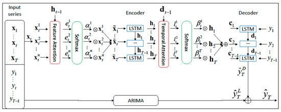
Figure 1.
Wear prediction model diagram.
The feature attention mechanism is first introduced to analyze the input data sequence, and the weights of each feature under the temporal condition are set based on the contribution of the prediction results, thereby obtaining the LSTM hidden state at the current time. Then, the temporal attention mechanism is introduced to perform weighted calculations on the hidden state information, analyze the correlation of the long time-series data on the wear degree, decode the analysis results, and output them. Finally, considering the low sensitivity of the input signal to the output feedback of the neural network model [27], Arima is used to linearly correct the prediction result and optimize the wear degree prediction result.
2.1. Encoder with Integrated Feature Attention Mechanism
Given a time series input matrix generated from a wear data set, the matrix is defined as , where each is a vector that contains features, i.e., . represents the length of the sequence matrix window, and represents the data size of the input sequence at time . With the first values of the target sequence and as inputs, this model aims to train and learn the mapping from the input sequence to the current value of the target sequence .
The encoder in this article uses LSTM units, and each LSTM unit has a storage unit state representation at time . The access to the storage unit is controlled by input gate , forget gate and output gate . The structure of the encoder is shown in Figure 2.
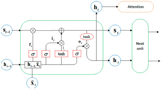
Figure 2.
Schematic diagram of the encoder structure.
The process of updating the hidden state of each encoder unit is represented by the following formula:
Among them, ( represents the size of the hidden state) represents the concatenation of the previous hidden state and the current input . and are the weight and bias terms that need to be learned. refers to the Sigmoid function and represents the element-wise multiplication at corresponding positions in matrices.
The prediction of the wear level in this article involves multiple factors such as torque, vertical force, turning angle, friction coefficient, and temperature, and there are complex correlation relationships between these features. In order to better grasp the inherent connections between the characteristics, this article uses a feature attention mechanism to adaptively select relevant feature sequences. The attention weight of the local features is obtained by referring to the LSTM unit’s previous hidden state and unit state . The formula for the constructed attention mechanism is as follows:
Among them, represents the -th input sequence within the step length, and are the weight and bias items that need to be learned.
Then, the Softmax function is applied to for normalization to obtain , represents the importance of the -th feature at time to the target sequence, and its calculation formula is as follows:
Calculate the weighted sum of all input feature sequences, and use it as the output . Then, the hidden state of the LSTM encoder unit at time can be updated, which is the nonlinear mapping from to :
2.2. Decoder with Integrated Temporal Attention Mechanism
The traditional encoder–decoder structure cannot capture long-term temporal relationships in input sequences. As the time series grows, the predictive performance of this structure will deteriorate significantly. To solve this problem, the temporal attention mechanism is introduced to perform weighted calculations on the hidden state information, analyze the long time-series correlation of the wear degree data, decode the analysis results, and finally output the prediction results .
The attention weights of each encoder’s hidden state at a given time are calculated based on the previous hidden state of the decoder and the storage state of the LSTM unit, as shown in the following Formula:
In Formula (10), represents the concatenation of the previous hidden state and unit state, and are the parameter weights and bias terms to be learned. The attention weight obtained after normalization using the Softmax function represents the importance of the -th encoder hidden state at time to the predicted target sequence. The weighted sum of the encoder’s hidden states is calculated to serve as the input to the corresponding decoder. The formula is as follows:
The decoder’s hidden state at time can be represented by combining with the given first target sequences, as follows:
The update formula for is similar to the update Formulas (2)–(5) of the encoder hidden states . The updated can be express as:
The mapping from input sequence to predicted target sequence value can be represented as:
represents their concatenation, parameter and map it to the size of the decoder’s hidden state, represents weight values, and represents bias terms. is the predicted wear result of the decoder output.
By analyzing the importance of different input positions through the temporal attention mechanism and adaptively optimizing the weight configuration, the adverse effects caused by information dilution during the input process are alleviated, and the predictive performance of the model for long time-series data is improved. Although the performance has improved, there is still room for optimization in predicting real-world data sets with large fluctuations.
2.3. Linear Autoregressive Component
Since various gates in the LSTM unit use non-linear activation functions to map input signals to output signals, these activation functions tend to approach zero derivatives when there is a large-scale change in input signals, resulting in a decrease in the learning rate of the gradient descent algorithm, slow updating of network parameters, difficulty in converging to the optimal solution [28], and a decrease in prediction accuracy.
To solve the above problem, this paper constructs a composite prediction model using the linear autoregressive moving average model (ARIMA) to correct the non-linear component and optimize the final prediction result. The ARIMA model construction process is shown in Figure 3.
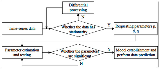
Figure 3.
ARIMA Model Construction Process.
The time series data used for wear prediction is non-stationary. Firstly, it is necessary to determine the order of differencing d to perform the differencing operation and conduct a stationarity test to obtain a relatively stationary time series. Then, the auto-correlation Function (ACF) and partial auto-correlation function (PACF) of the stationary time series are respectively calculated, and the corresponding order is obtained based on the autocorrelation and partial autocorrelation plots. Finally, the optimal order values p and q are obtained through parameter estimation to complete the construction of the ARIMA model. The prediction component obtained based on this model is represented as . The prediction result output by the overall composite model is shown below:
and are two hyperparameters. represents the linear prediction component and represents the non-linear prediction component.
The predicted results of the combination of linear components make up for the inherent deficiency of neural networks’ insensitivity to scale, allowing them to output more accurate predicted results at different scales of input sequences, thereby improving the model’s generalization ability and stability.
3. Experimental Design and Verification
3.1. Dataset Description and Preprocessing
Dataset 1: The bearing wear dataset used in this paper is obtained from a parts quality monitoring center located in Changchun, Jilin Province, China. This institution has a collaborative relationship with the School of Computer Science and Technology at Changchun University of Science and Technology. All the data were collected on the experimental platform provided by this institution. The experimental platform is shown in Figure 4. Part of the data set sequence is shown in Figure 5.
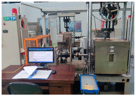
Figure 4.
Illustration of experimental platform.
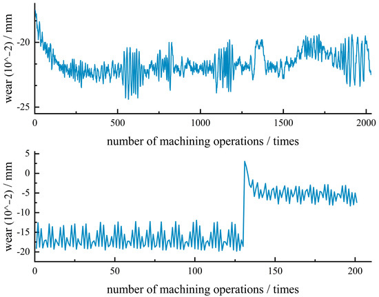
Figure 5.
Illustration of wear prediction sequence dataset.
The experimental bearings used are double-row radial ball bearings (SKF 2204E-2RS1TN9). An AC motor rotates at a constant speed of 3000 RPM and is connected to the bearings through a friction belt. The bearing material is high-carbon chromium bearing steel (GCr15) with an outer ring diameter of 47 mm, an inner ring diameter of 20 mm, a radial load of 11.5 kN, and a torque load of 0.7 N·m. The collected data consists of nine features: vertical force, jaw angle, torque, torque peak value, torque valley value, friction coefficient, bearing temperature, operating time, and wear amount. Torque is measured using a torque sensor with a range of 500 N·m. The jaw angle is measured using a wire encoder, and angular displacement (angular velocity) is detected using an optical encoder. The bearing wear amount is measured using a laser distance sensor. The force on the bearing is measured using a load sensor. The sampling frequency is set at 20 kHz, with measurements taken at regular intervals to capture the bearing wear amount. The collected data is divided into a 70% training set and a 30% testing set. This dataset is utilized in both Experiment 1 and Experiment 2.
Dataset 2: NASA Milling Cutter Wear Dataset [29]. This data is sourced from publicly available milling cutter wear experimental data conducted by NASA laboratories. The data collection was performed during dry milling and roughing operations under various cutting parameters and conditions. The experiment utilized six sensors, including two vibration sensors, two current sensors, and two acoustic emission sensors. The collected data consists of six features: table vibration, spindle vibration, AC spindle motor current, DC spindle motor current, acoustic emission at the table, and acoustic emission at the spindle. The sampling frequency was set at 100 kHz, resulting in a total of six-channel signals. A total of sixteen 6-flute milling cutters (KC710) were tested in the experiment. Each cutter was machined in a brand-new state, and the tool wear was measured using a microscope at regular intervals until the wear reached a certain level and the experiment was stopped. Two feed rates, 0.5 mm/rev and 0.25 mm/rev, which translate into 413 mm/min and 206.5 mm/min, and two radial cutting depths, 0.75 mm and 1.5 mm, were selected as milling parameters. The experiment included two types of tool materials: cast iron and stainless steel. This paper selected data from tools 3, 9, and 13 and created three test cases, C3, C9, and C13, respectively, for method validation, where C3 and C9 were used as the training sets and C13 was used as the testing set. This dataset is utilized in Experiment 3. Table 1 represents the processing conditions corresponding to three types of cutting tools.

Table 1.
NASA Milling Dataset tool processing conditions.
As mentioned in the introduction of this paper, industrial big data has many uses and can be applied in industrial modeling, prediction, control, decision-making, optimization, fault diagnosis, etc. However, the pursuit of stability and reliability in the industry sets high requirements for data quality in these applications. Specifically, data generated in industrial processes is prone to noise, missing values, and outliers due to sensor failures, human operational factors, and system errors. Using such data directly for analysis can have a severe negative impact on the accuracy and reliability of models. Therefore, prior to modeling, it is often necessary to preprocess the data, eliminating noise, correcting inconsistencies, and identifying and removing outliers, in order to enhance model robustness and prevent overfitting.
By visualizing the collected data samples, two main types of data defects can be identified: invalid data and outlier data. Invalid data typically occurs during the initial startup phase of the experimental platform. Since the dataset itself is large and the proportion of invalid data is relatively small, a direct deletion approach is employed to handle invalid data. On the other hand, outlier data in the dataset often manifests as sudden amplitude changes in one or several data points due to certain reasons. In this study, a sliding window median filtering method (Hampel filtering) is utilized for outlier data processing. The effect of outlier data and invalid data processing is shown in Figure 6. First, a sample size is set, and the window size is defined as . An upper and lower bound coefficient is specified. Subsequently, using a sliding window approach, the local standard deviation and the local estimated median are calculated for each sample. Finally, the upper and lower bounds for outlier detection are determined. Finally, the upper bound of outlier values is calculated as , while the lower bound is calculated as . If a sample value exceeds the upper bound or falls below the lower bound, it is replaced with the estimated median . There is no fixed standard for determining the value of the sliding window size. It is necessary to choose an appropriate window length based on the actual data characteristics and filtering effectiveness. In general, the higher the data sampling frequency and the more sampling points available, the larger the window length can be, and vice versa. If the data has a faster rate of change, the window length should be reduced accordingly to capture the data changes in a timely manner, while it can be increased if the rate of change is slower. A common rule of thumb is to choose a window size of around 5% to 15% of the length of the time data sequence. The usefulness of the procedure depends on the specific characteristics of the dataset and the goals of the analysis. Both limited and large datasets can benefit from the sliding window median filtering (Hampel filtering) procedure for handling outliers. With a limited dataset, sliding window median filtering can still be useful for identifying and mitigating outliers. It can help smooth the data and identify potential anomalies within the available observations. However, it is important to be cautious, as the effectiveness of the procedure may be limited by the small sample size. The statistical robustness of the results may decrease when the dataset is small. With a large dataset, sliding window median filtering can still be valuable for outlier detection and correction. It can provide a means to identify and handle outliers in a more efficient manner. Additionally, larger datasets often provide more reliable statistical estimates, which can enhance the accuracy of the sliding window median filtering process. In summary, while both limited and large datasets can benefit from the sliding window median filtering procedure, it is important to consider the limitations of the dataset size. A larger dataset generally provides more robust results and statistical estimates. However, even with a limited dataset, the procedure can still be useful for detecting and handling outliers, but the interpretability of the results should be approached with caution.
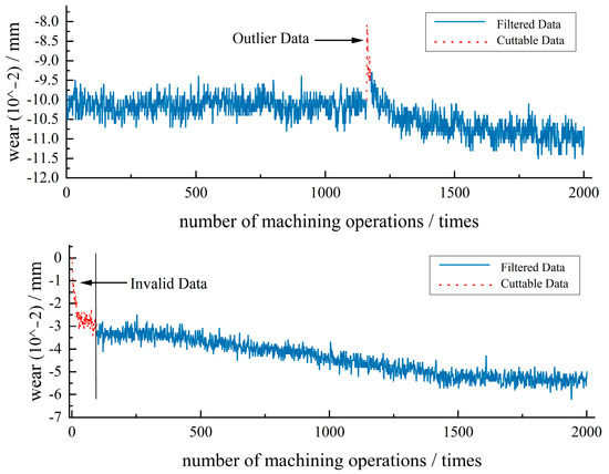
Figure 6.
Visualization of handling outlier data and invalid data.
By performing operations such as analysis and handling of invalid data, outlier localization analysis, and data filtering on the original data from the wear dataset, a solid foundation is established for the subsequent experiments.
3.2. Model Parameters
The experimental environment was configured with an AMD R5 5500U (2.10 GHz) and 16 GB of RAM. The programming language used was Python 3.6, and the deep learning experiments were completed using the TensorFlow framework. The parameter settings for the prediction model training are shown in Table 2. The setting of learning rates in Table 2 is manually determined based on empirical experience. If the learning rate is too large, it may not converge to the local optimal solution, while setting it too small can result in slow convergence of the model and potential overfitting. In this study, the initial learning rates are set to 0.1, 0.01, 0.001, 0.0001, etc., to observe the loss during the initial epochs of the network. Eventually, a learning rate of 0.01 is selected. The model reduces the learning rate by 5% every 10,000 iterations. The sensors record a total of nine features: vertical force, jaw angle, torque, torque peak value, torque valley value, friction coefficient, bearing temperature, operating time, and wear amount. The Adam algorithm was used as the optimizer for model training.
Table 2.
Forecast model parameter setting table.
3.3. Evaluation Metrics
When using a combined model for prediction and comparing the prediction performance of different models, this paper uses the following evaluation metrics: root mean square error (RMSE), mean absolute error (MAE), mean absolute percentage error (MAPE), and R2, corresponding to the calculation Formulas (18)–(21):
where represents the true value of wear at time , is the result obtained by the model prediction, and is the mean value of the true wear data.
3.4. Experimental Results and Analysis
Experiment 1: Performance analysis of an algorithm with an attention fusion mechanism.
Targeting the issue of low prediction accuracy for long-term sequential data in encoder–decoder architectures, the performance of the algorithm is improved by incorporating feature attention mechanisms and temporal attention mechanisms to handle long sequence information. To prove the effectiveness of the algorithm with the fusion of dual attention mechanisms, a comparative prediction experiment was conducted using a single attention mechanism and a dual attention mechanism, and the experimental results are shown in Table 3.
Table 3.
Performance comparison of models using different attention mechanisms.
From the data in Table 3, compared with the FA-Encoder-Decoder that uses the feature attention mechanism alone, the DA-Encoder-Decoder model has improved by 0.8113, 1.5848, 2.7314 (%), and 0.0389 in the four indicators of MAE, RMSE, MAPE, and R2, which confirms the significant gain of adding the temporal attention mechanism for predicting long-term sequence data. Compared with the TA-Encoder-Decoder that uses the temporal attention mechanism alone, the DA-Encoder-Decoder model has improved by 0.5546, 0.6157, 2.6773 (%), and 0.0256 in the four indicators, confirming the effectiveness of adding the feature attention mechanism to improve the prediction indicators. The visualized comparative results are shown in Figure 7, with the red line representing the model with the fusion of dual attention mechanisms, which has a higher degree of fit between the prediction curve and the true value compared to the other two models with single attention mechanisms. The reason for this is that the feature attention mechanism can adaptively select more important features according to the contribution of each feature to the wearer, while the temporal attention mechanism can solve the problem of diluted information caused by long sequence input. Therefore, the joint action of these two attention mechanisms has a better prediction effect.
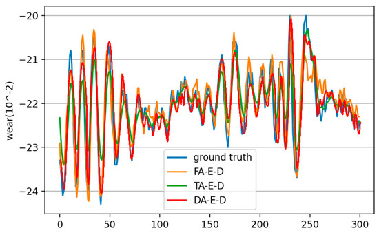
Figure 7.
Comparison of algorithms with fusion of different attention mechanisms.
Experiment 2: Performance validation of an algorithm with linear autoregressive component optimization.
In order to address the problem of neural network models being insensitive to input data with large-scale changes, the ARIMA linear model is introduced to optimize the prediction results. To verify the effectiveness of the improved combined prediction model, the long short-term memory network (LSTM), gated recurrent unit (GRU), and Stacked auto-encoder (SAEs) [30] were selected for comparative experiments. The dataset remained the same, and the experimental results are shown in Table 4.
Table 4.
Comparison of performance between combined prediction models and other basic algorithms.
From the data in Table 4, it can be seen that the DA-Encoder-Decoder prediction model with dual attention mechanisms is superior to the three basic neural network prediction models, LSTM, GRU, and SAEs, in four evaluation indicators. After introducing ARIMA, the DA + ARIMA combined prediction model can further improve the predictive ability by about 1.8%, 3.3%, 2.6%, and 1.6% on four evaluation indicators. The visualization comparison of the experiment is shown in Figure 8 and Figure 9. The figures intuitively indicate that under the conditions of drastic changes in input data scale, the prediction errors of the three basic neural network algorithms are relatively large. The prediction curve fitting effect of the dual attention mechanism model is improved, but the problem of error still exists. After introducing the linear component, the combined model exhibits the closest fitting accuracy between the prediction curve and the ground truth, effectively correcting errors. This indicates that neural network models may suffer from reduced sensitivity to changes in input signals and decreased prediction accuracy due to their nonlinear characteristics. The combination prediction model optimizes performance by incorporating linear prediction components, achieving the goal of improving wear degree prediction. The experimental results demonstrate its effectiveness.
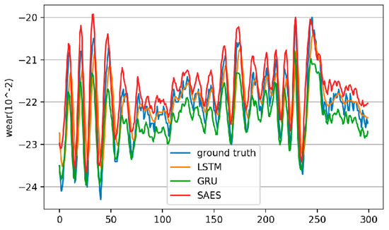
Figure 8.
Wear prediction results of LSTM, GRU, and SAEs.
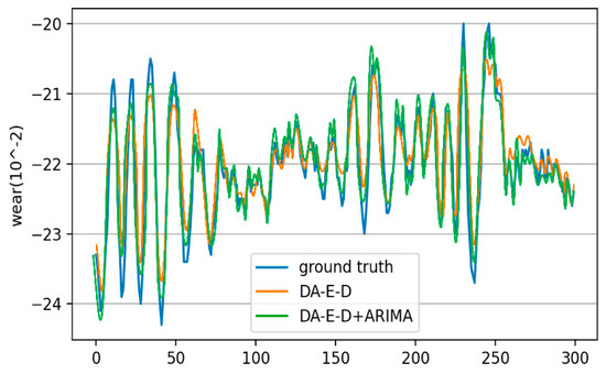
Figure 9.
Wear prediction results of the combination prediction model with added linear autoregressive component.
Experiment 3: Comparative experiments on the publicly available NASA dataset.
From Experiments 1 and 2, it can be observed that the proposed wear prediction method in this paper outperforms other baseline models significantly. This demonstrates the effectiveness of the trained model for wear prediction proposed in this study. Additionally, considering the limitation of a single dataset, in Experiment 3, the publicly available NASA milling tool wear data was used to predict tool wear under different conditions and parameters, further validating the effectiveness of the proposed method and confirming the conclusions drawn from the analysis. Furthermore, a comparative analysis was conducted between the algorithm studied in this paper and recent works on wear prediction, aiming to validate the universality and robustness of the algorithm.
In this section, the APCANet-MP-SVR (Activated PCANet with max pooling and support vector regression) model [31] and the SE-IDANN (sample expansion and improved domain adversarial training of neural networks) model [32] were used as comparative models. The APCANet-MP-SVR model improves tool wear prediction accuracy by optimizing the principal component analysis model (PCANet). The SE-IDANN model addresses the challenge of weak tool wear features by enhancing the domain adversarial neural network (DANN), enabling accurate prediction of tool wear quantity. The fitting curves of the comparative experiments on the NASA milling tool wear dataset are shown in Figure 10, and the results of the comparative experiments are presented in Table 5.
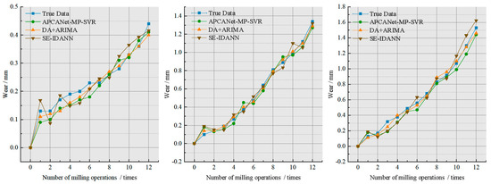
Figure 10.
Milling cutter wear prediction fitting curve of NASA.
Table 5.
Results of different methods in NASA dataset.
From the data in Table 5, the R2 values (used to measure the goodness of fit, where a value closer to 1 indicates better model performance) for different models on the dataset are all above 0.85, and the models demonstrated relatively stable accuracy in prediction. The DA + ARIMA model outperforms the APCANet-MP-SVR model and the SE-IDANN model in all three different test cases. The DA + ARIMA model achieves a 4.05%, 2.14%, and 4.02% higher R2 value than the APCANet-MP-SVR model and a 4.62%, 3.42%, and 4.52% higher R2 value than the SE-IDANN model in the respective test cases. Additionally, it can be observed that the DA-Encoder-Decoder model also exhibits slightly higher prediction performance compared to the two comparative models. The comparison metrics listed in Table 5 further validate the performance of the proposed model in this study, indicating its robustness.
4. Conclusions
To address the problem of poor long-sequence data prediction ability in the encoder-decoder structure for wear prediction analysis, a dual attention mechanism prediction model is proposed. The model integrates a feature attention mechanism to calculate the weight of each input feature at the current time and enhance the influence of important features on the prediction results. It also integrates a temporal attention mechanism to optimize the weighting of the hidden state information of the encoder and capture the long-term correlation of input data. To address the problem of low sensitivity of output feedback to input signal changes in neural networks, the ARIMA model is used to linearly correct the prediction results and further optimize the wear prediction results. The performance of the model with different attention mechanisms was tested on a real-world dataset, and a comparison experiment was designed between the combination prediction model and other prediction models. The results show that the combination prediction model has a significant advantage in improving wear prediction accuracy.
Author Contributions
Conceptualization, Z.W. and N.Q.; methodology, Z.W. and N.Q.; writing-original draft preparation, Z.W.; writing-review and editing, Z.W., N.Q. and M.L.; supervision, P.W.; project administration, P.W. All authors have read and agreed to the published version of the manuscript.
Funding
This research was funded by the Jilin Province Science and Technology Innovation Platform Construction Project (YDZJ202302CXJD027).
Institutional Review Board Statement
Not applicable.
Informed Consent Statement
Not applicable.
Data Availability Statement
The data is unavailable due to commercial restrictions.
Conflicts of Interest
The authors declare no conflict of interest.
References
- Liu, Q.; Qin, S. Perspectives on Big Data Modeling of Process Industries. Acta Autom. Sin. 2016, 42, 161–171. [Google Scholar]
- Ren, L.; Jia, Z.; Lai, L.; Zhou, L.; Zhang, L.; Li, B. Data-driven industrial intelligence: Current status and future directions. Comput. Integr. Manuf. Syst. 2022, 28, 1913–1939. [Google Scholar]
- Luo, L. Application and Practical Research of Industrial Big Data. Inf. Rec. Mater. 2022, 23, 167–169. [Google Scholar]
- Hu, D.; Zhang, C.; Wang, S.; Zhao, Q.; Li, J. Intelligent Prediction Model of Tool Wear Based on Deep Signal Processing and Stacked-ResGRU. Comput. Sci. 2021, 48, 175–183. [Google Scholar]
- Zhang, C.; Yao, X.; Zhang, J.; Liu, E. Tool wear monitoring based on deep learning. Comput. Integr. Manuf. Syst. 2017, 23, 2146–2155. [Google Scholar]
- Chen, Y.; Jin, Y.; Jiri, G. Predicting tool wear with multi-sensor data using deep belief networks. Int. J. Adv. Manuf. Technol. 2018, 99, 1917–1926. [Google Scholar] [CrossRef]
- Pahlavani, M.; Roshan, R. The comparison among ARIMA and hybrid ARIMA-GARCH models in forecasting the exchange rate of Iran. Int. J. Bus. Dev. Stud. 2015, 7, 31–50. [Google Scholar]
- Du, Y.; Li, W.; Li, H.; Liu, D. Structural Damage Identification Based on Time Series Analysis. J. Vib. Shock 2012, 31, 108–111. [Google Scholar]
- Wu, S.; Wei, Z.; Wang, S.; Wang, B.; Li, Y. Damage Identification Based on AR Model and PCA. J. Vib. Meas. Diagn. 2012, 32, 841–845+868. [Google Scholar]
- Liu, F.; Mao, Z. Dynamic Outlier Detection for Process Control Time Series. Control Theory Appl. 2012, 29, 424–432. [Google Scholar]
- Zhang, H.; Yin, Y.; Shen, H.; Zhang, M.; Wang, H. A Wind Speed Time Series Modelling Method Based on Probability Measure Transformation. Autom. Electr. Power Syst. 2013, 37, 7–10+17. [Google Scholar]
- Zhang, Y.; Wu, B.; Zhang, J.; Chen, W. Network Traffic Forecasting Based on Combined Model. J. Huazhong Univ. Sci. Technol. Nat. Sci. Ed. 2016, 44 (Suppl. 1), 29–34. [Google Scholar]
- Li, R.; Chen, W.; Xu, W.; Li, C. Prediction on the Value Trends of Bitcoin and Gold-on Account of ARMA Time Series Forecasting Model. Acad. J. Comput. Inf. Sci. 2022, 5, 79–84. [Google Scholar]
- Yang, J.; Liu, B.; Zhu, W.; Feng, C.; Zhang, H. Short-term Passenger Flow Prediction for Urban Rail Transit Based on Ensemble Models. J. Transp. Syst. Eng. Inf. Technol. 2019, 19, 119–125. [Google Scholar]
- Zhu, S.; Xia, H.; Lyu, X.; Lu, C.; Zhang, J.; Wang, Z.; Yin, W. Condition Prediction of Reactor Coolant Pump in Nuclear Power Plants based on the Combination of ARIMA and LSTM. Nucl. Power Eng. 2022, 43, 246–253. [Google Scholar]
- Li, Y.; Han, T.; Wang, J.; Quan, W.; He, D.; Jiao, R.; Wu, J.; Guo, H.; Ma, Z. Application of ARIMA Model for Mid-and Long-term Forecasting of Ozone Concentration. Environ. Sci. 2021, 42, 3118–3126. [Google Scholar]
- Shih, S.-Y.; Sun, F.-K.; Lee, H.-Y. Temporal pattern attention for multivariate time series forecasting. Mach. Learn. 2019, 108, 1421–1441. [Google Scholar] [CrossRef]
- Huang, Q.; Huang, H.; Zhang, Y.; Han, Y. Tool wear prediction based on multi-scale convolution attention network fusion. In Proceedings of the 2021 China Automation Congress, Beijing, China, 22–24 October 2021; Volume 6. [Google Scholar]
- Hu, J.; Zheng, W. Multistage attention network for multivariate time series prediction. Neurocomputing 2020, 383, 122–137. [Google Scholar] [CrossRef]
- Fu, E.; Zhang, Y.; Yang, F.; Wang, S. Temporal self-attention-based Conv-LSTM network for multivariate time series prediction. Neurocomputing 2022, 501, 162–173. [Google Scholar] [CrossRef]
- Abbasimehr, H.; Paki, R. Improving time series forecasting using LSTM and attention models. J. Ambient. Intell. Humaniz. Comput. 2022, 13, 673–691. [Google Scholar] [CrossRef]
- Du, S.; Li, T.; Yang, Y.; Horng, S.J. Multivariate time series forecasting via attention-based encoder–decoder framework. Neurocomputing 2020, 388, 269–279. [Google Scholar] [CrossRef]
- Pan, C.; Li, Z.; Yang, W.; Cai, L.; Jin, A. Anomaly Detection Method of Network Traffic Based on Secondary Feature Extraction and BiLSTM-Attention. J. Electron. Inf. Technol. 2023, 45, 1–9. [Google Scholar]
- Zhang, J. Aeroengine residual life prediction based on attention mechanism and CNN-BiLSTM model. J. Electron. Meas. Instrum. 2022, 36, 231–237. [Google Scholar]
- Zhao, H.; Huang, D.; Zeng, R.; Yu, J. Short-term traffic flow prediction based on spatio-temporal attention Bi-LSTM model. Comput. Simul. 2022, 39, 177–181+455. [Google Scholar]
- Sutskever, I.; Vinyals, O.; Le, Q.V. Sequence to sequence learning with neural networks. In Proceedings of the Advances in neural information processing systems, Montreal, QC, Canada, 8–13 December 2014; Volume 27. [Google Scholar]
- Lai, G.; Chang, W.C.; Yang, Y.; Liu, H. Modeling long-and short-term temporal patterns with deep neural networks. In Proceedings of the 41st International ACM SIGIR Conference on Research & Development in Information Retrieval, Ann Arbor, MI, USA, 8–12 July 2018; pp. 95–104. [Google Scholar]
- Sharma, S.; Sharma, S.; Athaiya, A. Activation functions in neural networks. Towards Data Sci. 2017, 6, 310–316. [Google Scholar] [CrossRef]
- Agogino, A.; Goebel, K. Mill Data Set [EB/OL]. Available online: https://ti.arc.nasa.gov/project/prognostic-data-repository (accessed on 1 February 2023).
- Chen, M.; Zeng, W.; Xu, Z.; Li, J. Delay prediction based on deep stacked autoencoder networks. In Proceedings of the Asia-Pacific Conference on Intelligent Medical 2018 & International Conference on Transportation and Traffic Engineering 2018, Beijing, China, 21–23 December 2018; pp. 238–242. [Google Scholar]
- Duan, J.; Zhou, H.; Liu, Z.; Zhan, X.; Liang, J.; Shi, T. Milling Tool Wear Prediction Research Based on Optimized PCANet Model. J. Mech. Eng. 2023, 59, 278–285. [Google Scholar]
- Dong, S.; Jiang, M.; Luo, Z. Tool status recognition method based on sample expansion and IDANN. J. Chongqing Univ. 2023, 46, 16–26. [Google Scholar]


Disclaimer/Publisher’s Note: The statements, opinions and data contained in all publications are solely those of the individual author(s) and contributor(s) and not of MDPI and/or the editor(s). MDPI and/or the editor(s) disclaim responsibility for any injury to people or property resulting from any ideas, methods, instructions or products referred to in the content. |
© 2023 by the authors. Licensee MDPI, Basel, Switzerland. This article is an open access article distributed under the terms and conditions of the Creative Commons Attribution (CC BY) license (https://creativecommons.org/licenses/by/4.0/).