Research on the Mobile Robot Map-Building Algorithm Based on Multi-Source Fusion

Abstract

In this paper, the mobile robot position fusion algorithm is inaccurate. There is a delay, and the map-construction accuracy is not high; an improvement method is proposed. First, the Cartographer algorithm is optimized. Radius filtering is used for data processing after voxel filtering. In contrast, the idea of multi-sensor fusion is used to fuse the processed IMU data information. This improved method improves the efficiency of the algorithm and the accuracy of the positional pose fusion. We verify the effect of the algorithm applied to the environment map, respectively, in the experimental building promenade environment and the teaching building hall environment, and analyze and compare the effect of map construction before and after the improvement; the experiment proves that in the experimental building promenade environment, the absolute error of measuring and analyzing the obstacles reduces by 0.06 m, and the relative error decreases by 1.63%; in the teaching building hall environment, the absolute error of measuring and analyzing the longest side of the map decreases by 1.121 m and the relative error decreased by 5.52%. In addition, during the experimental operation, the CPU occupancy of the optimized algorithm is around 59.5%. In contrast, the CPU occupancy of the original algorithm is 67% on average, and sometimes it will soar to 75%. The experimental results prove that the algorithm in this paper significantly improves performance in all aspects when constructing real-time environment maps.

1. Introduction

The problem of localization and map-building for mobile robots, which is the basis for achieving autonomous navigation, has become a hot research topic. To solve the indoor and outdoor localization problems and achieve accurate autonomous navigation, the robot map-building process—a single sensor—cannot complete complex map-building. In simultaneous localization and map-building (SLAM), fusing multiple sensors for map-building has become a popular research topic [1,2]. Traditional SLAM algorithms usually rely on a single sensor, such as LiDAR or a camera. Still, using a single sensor has some limitations [3]: vision sensors are susceptible to lighting conditions, while object reflections and occlusions limit LiDAR. To overcome these limitations, researchers have started to fuse multiple sensors to improve the accuracy and robustness of map-building [4].

Standard sensors include LiDAR, cameras, inertial measurement units (IMU), GPS, and more. LiDAR provides accurate distance and depth information. IMU can give information about robot attitude and acceleration, and vision sensors can provide visual information about the environment [5,6,7]. The choice of fused sensors depends on the specific application scenario and requirements [8]. The map-building algorithm for fusing multiple sensors involves techniques for calibrating sensor data, data correlation, and state estimation. Wei Shen et al. [9] proposed a USV LiDAR–slam-assisted fusion localization method that combines GNSS/INS localization with LiDAR–slam, which uses different sensor-fusion information and data-feedback correction to achieve the effect in different situations, and obtains data with more stability and observability. Xing Wei et al. [10] proposed an improved Hector–SLAM algorithm by finding that the Hector–SLAM algorithm has the problem of map drift and overlap when constructing maps, which first eliminates invalid laser data and then uses Inertial Measurement Unit (IMU) for compensation, and the method effectively improves the accuracy of the maps and the efficiency of the robot. Zhang Shaojiang et al. [11] proposed a map-matching method based on the combination of LiDAR, IMU, and an odometer for point-cloud data, which matches the point-cloud information collected by LiDAR with the known point-cloud data, introduces the point-to-point iterative closest-point algorithm (PP-ICP), and at the same time, the starting point of the autopilot car is set to be the initial coordinates of the point-cloud map data, and then establishes a predictive-state equation composed of the autopilot car’s gas-pedal control and steering wheel control of the self-driving car, then selects the predictive-state equations consisting of the throttle control and steering wheel control of the self-driving car. Finally, it utilizes the extended Kalman filter to fuse the information data from the three sensors, to update and correct the localization. Its robustness and localization accuracy meet engineering requirements, but on the other hand, it also increases the computational volume and difficulty of the algorithm. IMU-based fusion methods pose significant challenges in solving time synchronization and measurement delay problems. Researchers have been optimizing the Kalman filter update process to address this issue. Xia Xin et al. [12] proposed an algorithm for estimating the sideslip angle of self-driving cars based on the synthesis of consensus and vehicle kinematics/dynamics. Based on the measurement of the velocity error between the Reduced-Delay Inertial Navigation System (R-INS) and the Global Navigation Satellite System (GNSS), the velocity-based Kalman filter is formalized to estimate the R-INS velocity error, attitude error, and gyro bias error. Xin Xia and Lu Xiong et al. [13] fused the information from the Inertial Measurement Unit (IMU) and the Global Navigation Satellite System (GNSS) to align the heading of the GNSS and proposed a method for estimating the sideslip angle based on the vehicle kinematics model. Lu Xiong et al. [14] offered an adaptive Kalman filter low-sampling-rate Global Navigation Satellite System (GNSS) speed and position measurement method based on Inertial Measurement Unit (IMU). Liu Wei et al. [15] proposed a kinematic model-based VSA estimation method by fusing the information from Global Navigation Satellite System (GNSS) and Inertial Measurement Unit (IMU).

With the diversification and requirements of simultaneous localization and map-building application scenarios, academics have paid increasing attention to the development of SLAM algorithms [16]. Researchers are committed to designing efficient versions of SLAM algorithms suitable for different hardware platforms to meet the performance requirements in different environments and application scenarios [17], and graph-optimization algorithms are gradually being applied. Olson et al. [18] proposed an optimization method based on stochastic gradient descent (SGD), where iteratively, the non-repeatedly randomly selecting constraints and calculating the corresponding gradient descent direction, in which the optimal solution of the objective function is found, can effectively correct the bitmap. Grisetti et al. [19] extended Olson’s algorithm—a novel node parameterization is applied to the graph, which significantly improves the performance. The ability to handle arbitrary network topologies allows the binding of the complexity of the algorithm to the size of the mapping region rather than to the length of the trajectory. One of the most representative open-source SLAM algorithms for graph optimization is the Cartographer algorithm proposed by Google, which adjusts the bit pose of the submap on the path using loopback detection [20], thus removing the accumulated error in the process of building the graph from the last loopback to the current moment while achieving a balance between computational effort and real-time performance. In the literature [21], an adaptive multi-stage distance scheduler is used to optimize the processing speed of the Cartographer, and the local positional correction is achieved by controlling the scanning range of the LiDAR sensor and the search window of the point-cloud matcher through the scheduling algorithm. The algorithm effectively increases the processing speed of the Cartographer to a level similar to that of close-range LiDAR scanning while maintaining the accuracy of long-range scanning. Han Wang and Chen Wang et al. [22] introduced point-cloud intensity information into SLAM systems and proposed a novel SLAM framework by adding intensity constraints in the front-end odometry and back-end optimization phases, which uses frame-to-map matching to compute the optimal bit position by minimizing the geometric residuals and intensity residuals, which provides higher accuracy compared to purely geometric SLAM methods. Still, LOAM-based algorithms must perform downsampling operations of the point-cloud data in the execution phase, which does not accurately represent the underlying local network structure.

In the autonomous driving technology field, the sensors’ localization algorithm, one of the most basic and essential aspects, has received increasingly extensive attention [23]. With the continuous development of deep-learning technology, many scholars have now studied deep-learning-based SLAM schemes to obtain better accuracy and stronger robustness. Deep-learning-based SLAM technology has made many breakthroughs, especially in feature extraction, and matching has shown excellent performance [24]. Li Zhichao et al. [25] implemented geometric constraints in the odometry framework to decompose bit position estimation into two parts: the learning-based matching network part and the rigid transform estimation part based on singular value decomposition, and the experimental results show that the method has comparable performance with the traditional LiDAR odometry method. Liu Wei et al. [26] proposed a new algorithm, YOLOv5-tassel, which employs four detection heads and BiFPN to enhance feature fusion for small fringe detection, and introduces the attention mechanism of SimAM to extract the part of interest in feature mapping.

This study addresses the problem of local SLAM localization and map-building in indoor and outdoor environments, based on Google’s open-source Cartographer algorithm for improvement. In this paper, an improved voxel filtering and IMU information preprocessing method is proposed, and IMU information is introduced using the idea of multi-sensor fusion. The technique can be applied to mapping and navigation, and the experimental results verify the superiority of the algorithm of fused IMU information in constructing high-precision environmental maps.

2. Research of SLAM Algorithm

The Cartographer algorithm is a real-time map-construction algorithm capable of generating maps with a resolution of 0.05 m [27]. The algorithm is based on the principle of graph optimization, which graphically represents the process of robotic SLAM [28]. The optimization process is a nonlinear least-squares approach to optimize the cumulative error in building the map [29] to obtain a consistent map representation. The nodes in graph optimization represent the poses of the robot, while the edges represent the spatially constrained relationships between the nodes. Graph optimization is divided into two parts: front end and back end [30], while the optimization approach used in this paper is mainly applied to the front end. Figure 1 illustrates the infrastructure of the algorithm.

2.1. Submap

The usual scan-to-scan laser-matching accumulates errors. The Cartographer algorithm introduces the concept of submap, which turns the original scan-to-scan matching into scan-to-map matching, i.e., the laser matches with the submap first.

Several consecutive scans create a submap. When a submap is made, the raster probability is less than $P_{\min }$ for no obstacle at that point, between $P_{\min }$ and $P_{\max }$ for unknown, and greater than $P_{\max }$ for an obstacle at that point. Each frame of scans will generate a set of raster points called hits and a set of raster points called misses. Its submap is a raster map, and the submap can be considered a two-dimensional array whose value values under each index indicate the probability. To improve the performance and speed of operations, the Cartographer optimizes the probability representation.

As shown in Figure 2, the grid points in each hit are given the initial value $P_{\mathrm{hit}}$, and the grid points in each miss are called $P_{\mathrm{miss}}$. If the grid point already has a p-value, the value of the grid point is updated with the following.

The probability of a lattice probability p is defined as $odds\left(p\right)$.

$$odds\left(p\right)=\frac{p}{1-p}$$

(1)

$$M_{\mathrm{new}}\left(x\right)=clamp\left(\mathrm{odds}{}^{-1}\left(odds\left(M_{\mathrm{old}}\left(x\right)\right)·odds\left(P_{\mathrm{hit}}\right)\right)\right)$$

(2)

where clamp is the interval-limited function, $M\left(x\right)$ is the a priori lattice probability of the x under consideration. Each time, the latest scan obtained needs to be inserted into the optimal position in the submap so that when the bit pose of the point bundle in the scan is transformed and falls into the submap, each point has the highest confidence sum.

2.2. Local Slam

The front-end stage starts with data extraction, in which two methods, voxel filtering and adaptive voxel filtering, are used to compress the LiDAR data to reduce resource consumption and facilitate subsequent data processing. Due to the large scale of each frame of point-cloud data acquired by LiDAR and influenced by several factors, it can impact the point-cloud processing results. To estimate the trajectory and the bit position of the robot [31], an IMU and an odometer are used for extrapolation, and the estimated value of the bit position is used as the initial value. The LiDAR data are fused with the obtained positional estimates by a traceless Kalman filter [32] to update the positional estimates and to correct the LiDAR data. Each LiDAR scan forms a submap, and each frame of the point cloud is compared with the previous submap, and the pixel probability values in the submap are updated [33]. A motion filter is used to reject sensor frames of data at rest and continuously update the subgraph until a fully optimized subgraph is obtained when no new point clouds are inserted. The pseudo-code of the motion filter is as follows (Algorithm 1).

Algorithm 1: Motion Filter.

1: Input: Odometry, IMU, LaserScan   2: Output: Filtered motion estimation   3: Initialization:   4:     Initialize motion filter parameters   5:     Initialize state variables: pose, velocity, covariance matrix   6:     7: Procedure MotionFilter:   8: loop   9:     Receive Odometry, IMU, and LaserScan data 10:     Predict motion using odometry information 11:         Update state variables: pose, velocity 12:         Update covariance matrix based on the motion model 13:     Correct motion using IMU data 14:         Calculate IMU-based motion estimate 15:         Compare the estimated motion with the predicted motion 16:         Update state variables and covariance matrix based on the correction 17:     Fuse LaserScan data with motion estimate 18:         Perform scan-matching to align the laser scan with the estimated map 19:         Update state variables and covariance matrix based on the scan-matching result 20:     Output the filtered motion estimation 21: end loop 22:   23: End Procedure

The process uses a scan matcher based on the Ceres library to compute the poses of the point cloud, transforming the pose-solving problem into a nonlinear least-squares problem [34]:

$$\underset{{\Xi }^m,{\Xi }^s}{argmin}\frac{1}{2}\sum _{ij}\rho \left(E^2\left({\xi }_i^m,{\xi }_j^s;{\Sigma }_{ij},{\xi }_{ij}\right)\right)$$

(3)

where ${\Xi }^m=\left\{{\xi }_i^m\right\}$ are the coordinates of the submap in world coordinates; ${\Xi }^s=\left\{{\xi }_j^s\right\}$ is the locus of scan in world coordinates; ${\xi }_{ij}$ denotes the poses of the scan under the submap; ${\Sigma }_{ij}$ is the corresponding covariance matrix [35].

Residuals E and the error e:

$$E^2\left({\xi }_i^m,{\xi }_j^s;{\Sigma }_{ij},{\xi }_{ij}\right)=e{\left({\xi }_i^m,{\xi }_j^s;{\xi }_{ij}\right)}^T{\Sigma }_{ij}^{-1}e\left({\xi }_i^m,{\xi }_j^s;{\xi }_{ij}\right)$$

(4)

$$e\left({\xi }_i^m,{\xi }_j^s;{\xi }_{ij}\right)={\xi }_{ij}-\left(\begin{array}{c}{R}_{{\xi }_i^m}^{-1}\left(t_{{\xi }_i^m}-{\xi }_j^s\right)\\ {\xi }_{i;\theta }^m-{\xi }_{j;\theta }^s\end{array}\right)$$

(5)

First, during the loopback detection process, the system performs loopback optimization, i.e., it detects whether there is a loopback or not and then optimizes accordingly. When the current scan data are close enough in the distance to a certain laserscan position in the already created submap, the loopback can be found through a scan-matching strategy. To reduce the computation and improve the efficiency of real-time loop detection, Cartographer applies the branch-and-bound optimization method to optimize the search [36]. If a good-enough match is obtained, the loop-detection part is over by this point. The next step is to optimize the poses in all the submaps based on the current scan’s pose and one of the closest matches in the submap, even if the residual E is minimized.

In Equations (4) and (5), e is the error of optimizing the bit positions between the submap local and the submap global. Because there is a constraint on the bit positions of all the submaps, it is the optimization of the bit positions of all the submaps to minimize the error, as shown in Equation (5).

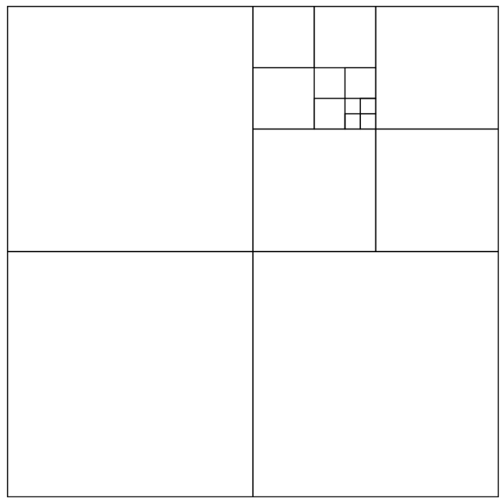
The subgraphs are inserted at the back end, the subgraphs are optimized using graph optimization, and the branch-delimitation method is used in the loopback detection process. The “branch-and-bound method” expands the feasible solution of a problem, like a branch of a tree, and then finds the best solution through each component. As shown in Figure 3.

Branch-and-bound aims to find the optimal pose of the newly built submap.

$${\xi }^{*}=\underset{\xi \in W}{argmax}\sum _{k=1}^K{M}_{\mathrm{nearest}}\left(T_{\xi }{h}_k\right)$$

(6)

$$W=\left\{{\xi }_0+\left(r{j}_x,r{j}_y,{\delta }_{\theta }{j}_{\theta }\right):\left(j_x,j_y,j_{\theta }\right)\in \overline{W}\right\}$$

(7)

$$\overline{W}=\left\{-w_x,\dots ,w_x\right\}\times \left\{-w_y,\dots ,w_y\right\}\times \left\{-w_{\theta },\dots ,w_{\theta }\right\}$$

(8)

where $M_{\mathrm{nearest}}$ first proximity to find the closest point and then expansion to the corresponding surrounding points; W is the search space; and ${\xi }_0$ is the center of the search space.

The branch-delimitation method performs cumulative error elimination [37], and each submap is matched with the corresponding bit pose to obtain the global map, i.e., the complete environmental map.

3. Cartographer Algorithm Improvement

Based on Google’s open-source Cartographer algorithm, this study improves and optimizes its front-end part to enhance the SLAM system’s performance in environment modeling and robot self-localization. In the front-end optimization, the focus is on processing point-cloud data and introducing the secondary filtering method of radius filtering after the voxel filter.

First, by applying the voxel filter, we effectively reduce the volume of the point-cloud data while retaining the critical feature information. However, after the voxel filtering process, the point-cloud data still has some diffusivity. To solve this problem, this paper adopts the secondary filtering method of radius filtering. The filtering effect is further improved by setting the threshold radius to filter out the point clouds that do not satisfy the conditions.

In the implementation process, the PCL library converts the point-cloud data to the format for the filtering operation. After converting the point-cloud data to the data format in the PCL library, the data can be processed using the rich filtering methods provided. After filtering, the data are converted back to the point-cloud data type required by the Cartographer algorithm to ensure compatibility with the subsequent SLAM algorithm.

In addition, this paper also preprocesses the IMU data and uses a multi-sensor-fusion method to fuse the processed IMU data with the point-cloud data. By combining the techniques of filter improvement and IMU data preprocessing, the accuracy and stability of the SLAM system for environment modeling and robot self-localization are improved.

Through these improvements and optimizations, this study aims to advance the performance of SLAM algorithms in practical applications and provide more accurate and reliable solutions for research and development in areas such as map construction and robot localization.

Figure 4 shows the flow chart of the improved algorithm.

3.1. Improved Voxel Filtering for Point-Cloud Preprocessing

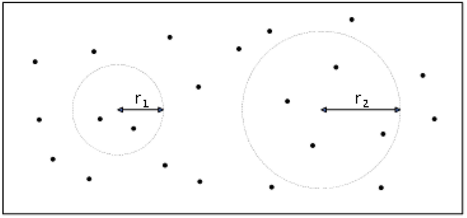
The purpose of point-cloud preprocessing is to simplify and reduce noise on point-cloud data to improve the operation efficiency of the algorithm and reduce the negative impact of noise in the subsequent scan-matching algorithm. Among them, radius filtering is a filtering method for filtering outliers. By setting thresholds for the filtering radius and the number of point clouds, the point clouds that do not meet the threshold conditions within the specified radius can be effectively filtered out. Using radius filtering, the speed of point-cloud preprocessing can be accelerated, and the algorithm’s efficiency can be improved. Such optimization measures help optimize the algorithm’s performance and make it more efficient and reliable in practical applications. The radius filtering is shown in Figure 5.

The steps to use the filtering algorithm are as follows:

1. Import the point cloud.

2. Filter type selection: Select the suitable filter type for the point cloud, commonly radius filter, statistical filter, Gaussian filter, etc. Each filter has different characteristics and applicable scenarios. Analyzing and comparing the advantages and disadvantages of the three filters, the radius filter is selected in this paper.

3. Parameter setting: According to the characteristics of the point cloud and the effect of filtering needed, set the filter parameters. For example, for the radius filter, you need to determine the radius size of the filter and decide the range of the filter search. In this paper, the parameters of the radius filter are selected after several iterative tests, and the relatively optimal radius of 5 and the minimum number of neighboring points of 100 are chosen.

4. Apply the filter: Use the filter to perform filtering operations on the point cloud. The filter will be calculated within a certain radius around each point in the point cloud to smooth or remove noise.

5. Handle boundary points: The point cloud may have boundary points, and you must choose an appropriate handling method. One standard practice is to leave the boundary points untreated, i.e., keep them in their original state; another way treats the boundary points, especially according to the filter type. This paper uses the first approach.

6. Filtering result output: After the filtering operation, the filtered point-cloud data are obtained, and the point-cloud data can be saved or subsequently analyzed and processed.

The pseudo-code for radius filtering is as follows (Algorithm 2):    

Algorithm 2: Radius filtering.

A radius filter can effectively remove noise and outliers, making the cloud data smoother and more consistent. The choice of filtering radius is crucial to the filtering effect; too small a radius may not remove all the noise, while too large a radius may lead to data loss or blurring. Therefore, selecting the appropriate radius value according to the specific application scenario and the characteristics of the point-cloud data is necessary before applying radius filtering.

3.2. IMU Preprocessing

First, noise-removal processing of IMU data is required [38]. Since environmental noise and interference may affect IMU data, noise removal of IMU data is necessary before the LiDAR map-building. Standard methods include mean filtering and Gaussian filtering.

Second, because of the time delay in IMU data, smoothing of the data is required to reduce the impact of the time delay on the bit-pose estimation. Commonly used methods include moving average filtering and exponential smoothing.

In the pose estimation of robots, the Kalman filter algorithm is usually used to estimate the poses based on IMU data [39]. To improve the accuracy and stability of attitude estimation, preprocessing IMU data is necessary. The Kalman filtering algorithm [40] is as follows:

Equation of state:

$${\widehat{x}}_{\overline{\mathrm{k}}}=A_{\mathrm{k}}{\widehat{x}}_{\mathrm{k}-1}+{\mathrm{B}}_{\mathrm{k}}{\mathrm{u}}_{\mathrm{k}}$$

(9)

Observation equation:

$${\mathrm{P}}_{\overline{\mathrm{k}}}={\mathrm{A}}_{\mathrm{k}}{\mathrm{P}}_{\mathrm{k}-1}{\mathrm{A}}_{\mathrm{k}}^{\mathrm{T}}+\mathrm{Q}$$

(10)

State update equation:

$${\mathrm{K}}_{\mathrm{k}}=\frac{{\mathrm{P}}_{\overline{\mathrm{k}}}{\mathrm{H}}_{\mathrm{k}}^{\mathrm{T}}}{{\mathrm{H}}_{\mathrm{k}}{\mathrm{P}}_{\overline{\mathrm{k}}}{\mathrm{H}}_{\mathrm{k}}^{\mathrm{T}}+\mathrm{R}}$$

(11)

$${\widehat{x}}_{\mathrm{k}}={\widehat{x}}_{\overline{\mathrm{k}}}+{\mathrm{K}}_{\mathrm{k}}\left({\mathrm{z}}_{\mathrm{k}}-{\mathrm{H}}_{\mathrm{k}}{\widehat{x}}_{\overline{\mathrm{k}}}\right)$$

(12)

$${\mathrm{P}}_{\mathrm{k}}=\left(\mathrm{I}-{\mathrm{K}}_{\mathrm{k}}{\mathrm{H}}_{\mathrm{k}}\right){\mathrm{P}}_{\overline{\mathrm{k}}}$$

(13)

In the above equation, the ${\mathrm{K}}_{\mathrm{k}}$ is the Kalman gain; ${\widehat{x}}_{\mathrm{k}-1}$ is the a posteriori state estimate at the moment $\mathrm{k}-1$, which is one of the filtering results, i.e., the updated result, also called the optimal estimate; ${\widehat{x}}_{\mathrm{k}}$ denotes the a priori state estimate at the moment k, and the predicted state at the moment k based on the optimal estimate at the moment $\mathrm{k}-1$; ${\mathrm{P}}_{\mathrm{k}-1}$ is the posterior estimate covariance at the moment $\mathrm{k}-1$; ${\mathrm{P}}_{\overline{\mathrm{k}}}$ is the prior estimate covariance at the moment k [41].

By noise removal and smoothing of IMU data, the quality and accuracy of the data can be improved to better utilize the IMU data to measure the robot’s positional information.

4. Laboratory Platform Construction

The software platform used in this paper is the PC and robot side, respectively, the PC side is the Ubuntu system, and the system version is Ubuntu 20.04, using the ROS system for operation. The version of ROS is noetic and packaged with Rviz and Gazebo (Rviz version 1.14.20; Gazebo version 11.11.0).

The LiDAR model is SLAMTEC S1, with a sampling speed of 9200 times/s, a scanning frequency of 10 Hz, a range resolution of 3 cm, and a measurement accuracy of 5 cm. The IMU model is WHEELTEC N100, a nine-axis attitude sensor for mobile robots. The sensor includes a three-axis gyroscope with a resolution of 0.02 degrees/s, a three-axis accelerometer with a solution of 0.5 mg, a three-axis magnetometer with a resolution of 1.5 Milligauss, and a thermometer. The baud rate of the serial port is 921,600 Bit/s. The robot side is the jetson nano main control board cart.

The distributed software architecture is shown in Figure 6.

Based on the robotics platform test, experiments were conducted in the long corridor on the third floor of the college building and in the lobby of the academic establishment. The scenes selected were large and simple to ensure the local maps would not have duplicate areas. The specific locations are shown in Figure 7.

The pictures above are of the corridor on the third floor and the lobby of the school building, respectively.

Laboratory Scenario Testing

A field run was performed on the robot, using the revo_lds.lua file that comes with the Cartographer algorithm to build the map and query the frame_id based on the LiDAR and the IMU hardware configuration.

The tf tree is shown in Figure 8 when fusing the IMU data.

The actual path when building the map on the third floor of the laboratory building is shown in Figure 9.

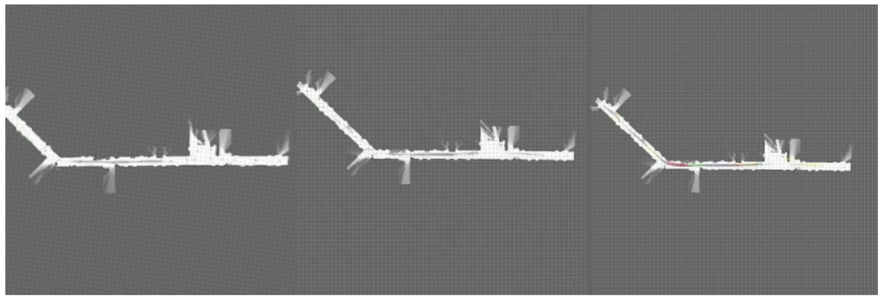
The following figure shows a scanned build of the robot in the third-floor corridor scene. After saving the map information, the 2D raster map is visualized on the PC side by rviz software.

Figure 10 shows the rendering effect of the laboratory corridor. The images from left to right show the rendering result of the original algorithm, the rendering mark of the original algorithm with IMU, and the rendering effect of the improved algorithm with IMU; Figure 11 shows the architectural impact of the teaching building lobby and the images from left to right are shown as above. The figure shows that after the effect is applied, the scanned map is more accurate than the original map, and the effects increase in sequence.

5. Experimental Data Analysis

5.1. Experimental Data

According to the experiment, eight locations of the longest edge of the map, the second-longest edge, the wide edge, the width of the connecting corridor, the width of the hall, and the length of the obstacle were selected to mark and measure the data, respectively. The approximate locations are shown in Figure 12 and Figure 13.

Table 1. Original algorithm test data in Figure 12.

Location	Actual Value/m	Measured Value	Absolute Error/m	Relative Error/%
1	52.51	53.01	0.5	0.95
2	25.053	25.456	0.403	1.61
3	1.97	2.12	0.15	7.61
4	2.718	2.83	0.112	4.12
5	6.055	6.01	0.045	0.74
6	3.688	3.87	0.182	4.93
7	2.865	2.82	0.045	1.57
8	0.94	0.89	0.05	5.32

Note: 1 (The longest side of the map), 2 (Map Sub-Long Edge), 3 (Map broadside). 4 (width of the corridor), 5 (Hall width), 6 (Obstacles), 7 (Width of building entrance), 8 (Door frame width).

,

Table 2. Original algorithm fusion inertial guidance test data in Figure 12.

Location	Actual Value/m	Measured Value	Absolute Error/m	Relative Error/%
1	52.51	52.92	0.41	0.78
2	25.053	25.398	0.345	1.38
3	1.97	2.12	0.15	7.61
4	2.718	2.825	0.107	3.94
5	6.055	6.016	0.039	0.64
6	3.688	3.866	0.178	4.83
7	2.865	2.83	0.035	1.22
8	0.94	0.897	0.043	4.57

Note: 1 (The longest side of the map), 2 (Map Sub-Long Edge), 3 (Map broadside), 4 (width of the corridor), 5 (Hall width), 6 (Obstacles), 7 (Width of building entrance), 8 (Door frame width).

and

Table 3. Optimized algorithm fusion inertial guidance test data in Figure 12.

Location	Actual Value/m	Measured Value	Absolute Error/m	Relative Error/%
1	52.51	52.79	0.28	0.53
2	25.053	25.23	0.177	0.71
3	1.97	2.11	0.14	7.11
4	2.718	2.796	0.078	2.9
5	6.055	6.09	0.035	0.58
6	3.688	3.81	0.122	3.3
7	2.865	2.838	0.027	0.94
8	0.94	0.958	0.018	1.9

Note: 1 (The longest side of the map), 2 (Map Sub-Long Edge), 3 (Map broadside), 4 (width of the corridor), 5 (Hall width), 6 (Obstacles), 7 (Width of building entrance), 8 (Door frame width).

show the experimental results’ test data in the third-floor corridor; The selected positions are 1—the longest side of the map, 2—map sub-long edge, 3—map broadside, 4—width of the corridor, 5—width of the hall, 6—the obstacles, 7—width of building entrance, and 8—width of the door frame.

Table 4. Original algorithm test data in Figure 13.

Location	Actual Value/m	Measured Value	Absolute Error/m	Relative Error/%
1	20.325	21.45	1.125	5.54
2	15.455	15.732	0.277	1.79
3	6.615	6.896	0.281	4.25
4	2	2.01	0.01	0.5
5	5.38	5.16	0.22	4.09
6	0.6	0.578	0.022	3.67
7	1.99	2.02	0.03	1.51
8	1.7	1.68	0.02	1.18

Note: 1 (The longest side of the map), 2 (Map Sub-Long Edge), 3 (Map broadside), 4 (Obstacles), 5 (U-shaped sofa length), 6 (U-shaped sofa width), 7 (O-shaped sofa width), 8 (Door frame width).

,

Table 5. Original algorithm fusion inertial guidance test data in Figure 13.

Location	Actual Value/m	Measured Value	Absolute Error/m	Relative Error/%
1	20.325	20.634	0.309	1.52
2	15.455	15.637	0.182	1.18
3	6.615	6.67	0.055	0.83
4	2	2.008	0.008	0.4
5	5.38	5.33	0.05	0.93
6	0.6	0.583	0.017	2.83
7	1.99	2.014	0.024	1.21
8	1.7	1.683	0.017	1

Note: 1 (The longest side of the map), 2 (Map Sub-Long Edge), 3 (Map broadside), 4 (Obstacles), 5 (U-shaped sofa length), 6 (U-shaped sofa width), 7 (O-shaped sofa width), 8 (Door frame width).

and

Table 6. Optimized algorithm fusion inertial guidance test data in Figure 13.

Location	Actual Value/m	Measured Value	Absolute Error/m	Relative Error/%
1	20.325	20.329	0.004	0.02
2	15.455	15.57	0.115	0.74
3	6.615	6.657	0.042	0.63
4	2	2.004	0.004	0.20
5	5.38	5.369	0.011	0.20
6	0.6	0.589	0.011	1.83
7	1.99	2.01	0.02	1.01
8	1.7	1.694	0.006	0.35

Note: 1 (The longest side of the map), 2 (Map Sub-Long Edge), 3 (Map broadside), 4 (Obstacles), 5 (U-shaped sofa length), 6 (U-shaped sofa width), 7 (O-shaped sofa width), 8 (Door frame width).

show the experimental results’ test data in the teaching building’s lobby; The selected positions are 1—the longest side of the map, 2—map sub-long edge, 3—map broadside, 4—obstacles, 5—U-shaped sofa length, 6—U-shaped sofa width, 7—O-shaped sofa width, 8—door frame width. The actual value is the map length, and the mapping measurement is the maximum value of the point-cloud boundary minus the minimum value [42].

5.2. Experimental Data Analysis

This study explores the error performance of the original algorithm, the original algorithm fused with inertial sensors, and the improved algorithm fused with inertial sensors in three cases by analyzing and comparing the absolute and relative error data in Table 1, Table 2, Table 3, Table 4, Table 5 and Table 6. This error performance aims to explore and illustrate the accuracy of constructing real-time maps; simultaneously, the algorithm’s requirement for computational resources of computer and robot hardware is another important criterion for judging map construction and localization algorithms. Computational power consumption can illustrate the algorithm’s efficiency in constructing real-time maps, measured by observing the CPU occupancy when running the algorithm. By monitoring the CPU occupancy during the execution of the algorithm, it is possible to determine the algorithm’s ability to process data promptly and, therefore, its ability to build and update maps under real-time constraints.

The selected positions in Table 1, Table 2 and Table 3 are used as horizontal coordinates, and the absolute errors are used as vertical coordinates to draw Figure 14, a table of absolute errors for the construction of the corridor of the laboratory building; and Figure 15, a table of relative errors for the construction of the corridor of the laboratory building, is drawn using the selected positions in Table 1, Table 2 and Table 3 as horizontal coordinates, and the relative errors are used as vertical coordinates. The positions chosen in Table 4, Table 5 and Table 6 are used as horizontal coordinates, and the absolute errors are used as vertical coordinates to draw Figure 16, a table of absolute errors for the construction of the hall of the teaching building; the selected positions in Table 4, Table 5 and Table 6 are used as horizontal coordinates, and the relative errors are used as vertical coordinates to draw Figure 17, a table of relative errors for the construction of the hall of the teaching building.

Figure 14 and Figure 15 show the absolute and relative error variation in the three cases during the laboratory corridor building process. As seen in Figure 14, in the method of measuring the longest side of the map, the absolute error of the original algorithm deviates the most from the absolute error of the original algorithm incorporating inertial sensors and the improved algorithm incorporating inertial sensors. The original algorithm suffers from the long and straight corridor effect [1]—due to the similarity and lack of diversity of features on both sides of the corridor, and the algorithm cannot accurately distinguish and build an accurate map, resulting in decreased map-building accuracy. In the experiments of this paper, it was mitigated and solved by adjusting the parameters, increasing the diversity of sensor data, and improving the algorithm. The absolute error was reduced from the original 0.5 m to 0.41 m after fusing the sensors and then to 0.28 m after the improved algorithm fusing the inertial sensors; the relative error was also reduced from the original 0.95% to 0.53%. In measuring and analyzing the length of the obstacle, the absolute error decreased from 0.182 m to 0.122 m, and the relative error also decreased by 1.63%.

As summarized in Figure 14 and Figure 15, the error curve of the original algorithm is consistently higher than the error curve of the original algorithm fusing inertial sensors and higher than the error curve of the improved algorithm fusing inertial sensors.

Figure 16 and Figure 17 show the changes in absolute and relative errors in the three cases during the map-building of the lobby of the teaching building. As seen in Figure 17, the original algorithm’s relative error curve fluctuates the most. In contrast, the curve of the improved algorithm incorporating inertial sensors fluctuates the least, can maintain better accuracy, and is the most stable. The lower relative error indicates that the algorithm can build the map more accurately and with less deviation relative to the accurate map.

According to Figure 14 and Figure 15 results, the performance is significantly better than the case without fused sensors by keeping the original algorithm unchanged and combining inertial sensors. When measuring the longest edge of the map, the absolute error is reduced from 0.5 m to 0.41 m, and the relative error is also reduced from 0.95% to 0.78%, which will mitigate the long and straight corridor effect. In addition, according to the results in Figure 16 and Figure 17, the improved algorithm reduces the absolute error of U-shaped couch length from 0.05 m to 0.011 m and the relative error from 0.73% while keeping the fused inertial sensors unchanged, which significantly improves the performance and makes the algorithm more stable. A comprehensive analysis of the results in Figure 14, Figure 15, Figure 16 and Figure 17 shows that after fusing inertial sensors, the Cartographer algorithm outperforms the original Cartographer algorithm.

In addition, during the experimental run, the CPU occupancy of the optimized algorithm is around 59.5%, while the CPU occupancy of the original algorithm is 67% on average, and sometimes soars to 75%. Overall, after improving the filtering algorithm, the fusion of inertial sensors for map-building will further improve the map-building effect. Overall, the performance of the optimized algorithm is significantly improved [43], and the optimized maps are straighter and squarer and have fewer distorted regions as seen from the outer frame of the maps.

6. Conclusions

In this paper, a new map-building algorithm is proposed for the inaccuracy of Cartographer algorithm position fusion, the existence of dense point-cloud data with high computational volume, and the low accuracy and efficiency of map construction. To reduce the diffusivity of the point-cloud data after voxel filter processing, this paper adopts the secondary filtering method of PCL library radius filtering. By setting the thresholds for the filter radius and the number of point clouds, the point clouds that do not satisfy the threshold conditions within the specified radius range are effectively filtered out, accelerating the speed of point-cloud preprocessing and improving the algorithm’s efficiency. At the same time, the multi-sensor-fusion method is adopted to fuse the IMU data information with the algorithm after preprocessing to enhance the effectiveness of the front-end map construction and the back-end loopback detection and ultimately to realize the construction of high-precision maps. By comparing and analyzing the experimental results of the original algorithm and the improved algorithm to construct the map, in the environment of the long corridor of the experimental building, the absolute error of measuring and analyzing the obstacles is reduced by 0.06 m, and the relative error is decreased by 1.63%; in the environment of the hall of the teaching building, the absolute error of measuring and analyzing the longest side of the map is reduced by 1.121 m. The relative error is decreased by 5.52%. In addition, during the experimental run, the CPU occupancy of the optimized algorithm is around 59.5%, while the CPU occupancy of the original algorithm averages 67% and sometimes spikes to 75%. This paper concludes that the fusion of inertial sensors based on the improved algorithm can improve the efficiency and accuracy of map-building. This paper concludes that the fusion of inertial sensors based on improved algorithms can improve the efficiency and accuracy of map-building.

In the future, in addition to the algorithms in this paper, there are sub-tasks such as loopback detection, position recovery, and sliding window optimization that plays an optimization role for map-building and localization in SLAM tasks—integrating these sub-tasks in the priority definition algorithm and network inference model to reach multi-task joint learning and realize the unity of multi-modal, multi-task, and real-time. Joint multi-task learning with correlation can also improve the performance of localization and map-building, which is one of the sub-directions worth studying.