Photoplethysmographic Signal-Diffusive Dynamics as a Mental-Stress Physiological Indicator Using Convolutional Neural Networks

Abstract

Stress is one of the primary triggers of serious pathologies (e.g., depression, obesity, heart attack). Prolonged exposure to it can lead to addictive substance consumption and even suicide, without ignoring other adverse side effects in the economic, work and family spheres. Early detection of stress would relax the pressure of medical practice exercised by the population affected and result in a healthier society with a more satisfying quality of life. In this work, a convolutional-neural-network (CNN) model is proposed to detect an individual’s stress state by analyzing the diffusive dynamics of the photoplethysmographic (PPG) signal. The characteristic $(p,q)$-planes of the 0–1 test serve as a framework to preprocess the PPG signals and feed the CNN with the dynamic information they supply to typify an individual’s stress level. The methodology follows CRISP-DM (Cross Industry Standard Process for Data Mining), which provides the typical steps in developing data-mining models. An adaptation of CRIPS-DM is applied, adding specific transitions between the usual stages of deep-learning models. The result is a CNN model whose performance amounts to 97% accuracy in diagnosing the stress level; it compares with other published results.

1. Introduction

The pace of life in today’s society tends to be increasingly unbridled and highly competitive, especially in large cities. These circumstances contribute to the fact that stress triggers have worsened over the years [1]. When stress is persistent and prolonged over time, it can lead to severe psychological disorders, such as anxiety or depression and also physiological disorders, such as obesity, due to poor eating behaviors, cardiovascular diseases, hypertension, low-back pain, ulcers, multiple sclerosis, diabetes, cancer risk and stroke, among others [2,3], substantially worsening the quality of life of an individual and their psychological well-being, leading in the most extreme cases to suicide, according to data reported by the World Health Organization [4]. Likewise, numerous investigations show the relationship between stress, acute or chronic, and addictive substances [5] or the appearance of infectious diseases [6]. Due to stress, the costs it entails for society acquire a non-negligible magnitude [7]. The estimated cost to the global economy of depression and anxiety in terms of productivity amounts to a trillion dollars a year [8].

1.1. Stress Overview

The notion of stress has faded over time as it has been used indiscriminately to precisely describe the physiological response to stress, the stimulus–response interaction or, globally, all the factors involved (e.g., stimulus, perception, the form of adaptation) [9]. Hans Selye defined stress in 1950 as a state of biological activation triggered in an individual when interacting with external agents that force his ability to adapt [10]. According to Richard S. Lazarus, stress also refers to an alteration of an individual’s homeostatic balance (physiological systems) that causes a stress response, which is nothing more than the body’s attempt to cope with the stressor [11]. The World Health Organization (WHO) associates stress with physiological reactions that prepare the body for action. A stressful factor or stressor is any element that leads to the physiological reaction to stress. They can be natural objects perceived as stressors by the individual, for example, a weapon, or situations internally perceived as uncertain or potentially threatening. The intensity of the physiological reaction to stressful factors highly depends on the individual and the specific situation. However, even with the multiple dimensions that stress eventually spans in its clinical spectrum, a generic description of stress that encompasses practically all those factors that intervene “grosso modo” in a stressful episode responds to “tension, mental or physical, caused by overwhelming situations (stressing factors) that cause psychosomatic reactions or psychological disorders, sometimes very serious, in order for the individual to adapt or cope with them” [12].

Stress can be classified as acute or chronic [13]. Acute stress comprises the immediate response of the body to a stressor in order to achieve a state adaptive to the stimulus and to survive; as soon as the stressor is gone, the bodily imbalance ceases to exist. However, chronic stress is one in which the stressful stimulus does not disappear quickly and the state of stress can last for a not insignificant period, such as months or even years.

Stress has become an endemic disease that affects everyone equally, regardless of age, origin or condition. The origin of stress is very varied and manifests itself in many daily situations, whether in the workplace, academic settings or family. It can be traumatic in response to adverse events, such as a natural catastrophe, war or serious accident, or as a result of an adverse event, such as job loss or illness. In this sense, innumerable studies link stress with the COVID-19 pandemic [14] or the harmful reactions that work stress entails for the body [15]. New stressors are generally perceived as more stressful and the physiological response tends to be more intense [16].

Positive or motivating reactions are effective in the short term when faced with low levels of acute stress. Such reactions can help individuals manage situations where they are under pressure, such as during an exam or job interview. Research has shown that prolonged exposure to acute stress can negatively impact motor-skill performance and pose a risk to physical and mental health and personal safety [9]. Chronic stress further aggravates its incidence in the body, causing more severe disorders, such as hypertension, obesity, diabetes, deficiencies in the immune system and cancer that do not go away when the stressor stops. The care of the terminally ill, long-term unemployment, economic problems, post-traumatic stress of war veterans and work overload illustrate chronic stress.

Stress control is entrusted to the autonomic nervous system (ANS), triggering a set of bodily changes of all kinds (e.g., hormonal, immunological, physiological, psychological) to counteract the stressful stimulus and thus restore the original homeostatic state [17]. Simply put, when encountering a stressful situation, whether short term or long term, the body responds by triggering various physical indicators. These include elevated glucose levels, heightened heart rate, wider opening of coronary vessels, narrowed peripheral blood vessels, dilated pupils and increased sweating. Early recognition of these indicators would help stop its progress and, perhaps, irreversible damage that would inexorably affect the well-being and health of society.

1.2. Stress Diagnosis

To accurately and consistently measure stress levels, a method must involve analysis of specific electrophysiological, biochemical and psychometric parameters, monitoring the subject’s development over time and examining the type and aspects of the stressor [18]. This work focuses exclusively on the electrophysiological parameters the photoplethysmographic (PPG) signal provides.

In the last decade, the diagnosis and preliminary clinical analysis of an individual’s state of health have been supported by non-invasive methods of monitoring biological signals [19]. The PPG signal deserves special attention, given its easy acquisition with affordable devices and the amount of physiological information it contains [20].

The PPG signal represents the volumetric variation experienced by the blood flow in the microvascular circulation of the tissues [21]. Photoplethysmography or photoplethysmogram (PPG) is an electro-optical technique that makes it possible to measure said volumetric variation in a barely invasive way and with minor sensitivity to the location of the sensors [20,22]. The dynamics of blood flow or hemodynamics through the peripheral capillary network can be an ideal candidate to accurately detect the state of stress or relaxation (non-stress) of an individual.

The first photoplethysmograph or pulse oximeter, attributed to the physiologist Alrick Hertzman, dates from 1937. Technological advances have led to the commercialization of increasingly economical pulse oximeters, of smaller size and lighter weight [23,24], giving them tremendous versatility for their application in very different areas, such as health, sports or the agri-food industry [25]. Likewise, its use has been extended to the clinical environment to monitor physiological parameters related to the cardiorespiratory system [26]. Unlike other biological signals, which require bulky equipment or multiple accessories, such as the use of gels in EEG (Electroencephalogram) signals or electrodes in ECG (Electrocardiogram) signals or GSR (Galvanic Skin Response) signals, PPG signals use reduced electronics that have favored the proliferation of small pulse oximeters with low-cost sensors and easy integration with other smart devices [27].

In our technology-driven world, Big Data has seen a significant increase in capabilities due to the availability of tools for collecting vast amounts of data. Within the clinical field, there exist large public databases containing a vast number of biological samples from both healthy individuals and those with various pathologies. These samples are organized by age range for ease of access. It is common to come across simple technological solutions that use biological signals to communicate a subject’s physiological characteristics. By conducting a thorough examination of biological signals, including the PPG signal, using advanced techniques, like those described in studies by Toker et al. (2020), Wu et al. (2022) and Park et al. (2022) [28,29,30], we expect to uncover more functional nuances of the physiological system that generates these signals over time.

In order to fully comprehend how a complex system is functioning, it is crucial to examine the dynamic correlation structures and fluctuations, also known as intrinsic vibrations, in the data [31]. This requires techniques capable of detecting local and global details during dynamic transitions at various time scales, as highlighted by [32,33,34]. In recent years, the field of Deep Learning (DL) and its applications have broken into innumerable fields, such as natural language processing, information processing, more education, cybersecurity, robotics and control, among others. Many scientific findings support convolutional neural networks’ (CNNs)’ benefits, either via deep or shallow methods [35,36]. In health, especially in clinical settings, techniques based on DL, given their versatility, precision, flexibility and high performance, have provided satisfactory results in processing large amounts of data based on biomedical signals [37,38].

1.3. Work Aims

This work aims to create and test a model that can accurately determine an individual’s stress level using PPG signals—data extracted from a national project. The model is compared with studies using machine-learning techniques to detect stress through different biological signals. Typically, the biological markers used to diagnose stress rely on the shape of biological signals. These signals can be easily affected by temporary changes in an individual’s physical activity or mindset and can also vary depending on the timing of the measurement. As a result, these markers may not accurately reflect the level of stress a person is experiencing.

This paper is focused on analyzing the geometric distribution of the dynamics or diffusive behavior of the PPG signal. We will use the $(p,q)$-plane suggested by the 0–1 test [39,40,41] to achieve this. Based on the two-dimensional structure of this distribution, equivalent to an image, we propose a model that utilizes DL to automate stress detection in a subject. In the last decade, CNNs have experienced a notable expansion, with magnificent results in the field of computer vision, in particular, in image recognition. Its proven reliability in image classification tipped the balance in its favor when choosing the neural network (NN) model we could implement. The promising results produced by this work further confirm its leading role.

It is essential to mention that before this work, no method had been proposed to identify stress based on the PPG signal considering the diffusion dynamics of the unique signal of each individual. The uniqueness of the dynamics is because the structure of each person’s vascular bed affects the diffusion constant of blood flow.

The proposed formulation will allow a highly portable system sensor crucial in certain risky professions, such as truck drivers, pilots and factory workers, among others, with a neural network of low weight in terms of memory consumption and efficiency above 90% in detecting acute stress.

In addition, the proposed method can be generalized in the state-of-the-art artificial intelligence classifiers—our proposal uses a conventional CNN—as a method of classifying time series via prior conversion to the $(p,q)$-plane.

The rest of the paper is organized as follows. Section 2 describes the proposed convolutional neural network architecture, supported by an analysis of the PPG signal-diffusive behavior, as well as the metrics to evaluate its performance. Section 3 shows the obtained results, both graphically and numerically, regarding the metrics that allow to judge the capacity of the neural network to distinguish a stressed state in a subject. In Section 4, we analyze and interpret the obtained results and provide a comparative analysis of these findings with other relevant studies. Finally, in Section 5, we shortly outline the conclusions drawn from this study, which serve as the basis for future work.

2. Materials and Methods

The approach to designing the model that assesses stress is based on the well-known CRISP-DM (Cross Industry Standard Process for Data Mining) methodology, as described by Chapman et al. (2000) [42]. Then, regarding image classification, it uses CNNs as a learning technique due to their remarkable capabilities in machine vision. After preprocessing the PPG signals, a two-dimensional Euclidean spatial transformation (using the series of Fourier transforms) is performed to obtain multiple $(p,q)$-planes. The 0–1 test suggested this method [39,40,41,43]. The input information to our model comprises a massive set of $(p,q)$-planes, two-dimensional planes that characterize the diffusive dynamics of PPG signals. Their stability and robustness against morphological changes of the PPG signal make this model a suitable alternative for determining a stressful episode.

To better understand the applied model and the results, the database is described in Section 2.1. Next, in Section 2.2, the CNN design architecture is explained and in Section 2.3, the parameters used to evaluate the model are enumerated.

2.1. PPG Signal

The original PPG signals used in this work come from 40 students from the UPM (Universidad Politécnica de Madrid), healthy young people between the ages of 18 and 30, who participated in a study of a national investigation that tried to evaluate the degree of incidence of mental stress in different biological signals. The volunteers declared that they were not habitual consumers of psychotropic substances and accredited the absence of a diagnostic history of chronic disease and/or psychopathologies. Through quota sampling, compliance with gender parity was satisfied, 50% men and 50% women [12,18]. Signals were captured from the middle finger of the left hand and sampled at a frequency of 250 Hz [18], with the psychophysiological telemetric system “Rehacor-T” version “Mini” from Medicom MTD Ltd., Taganrog, Russia [18].

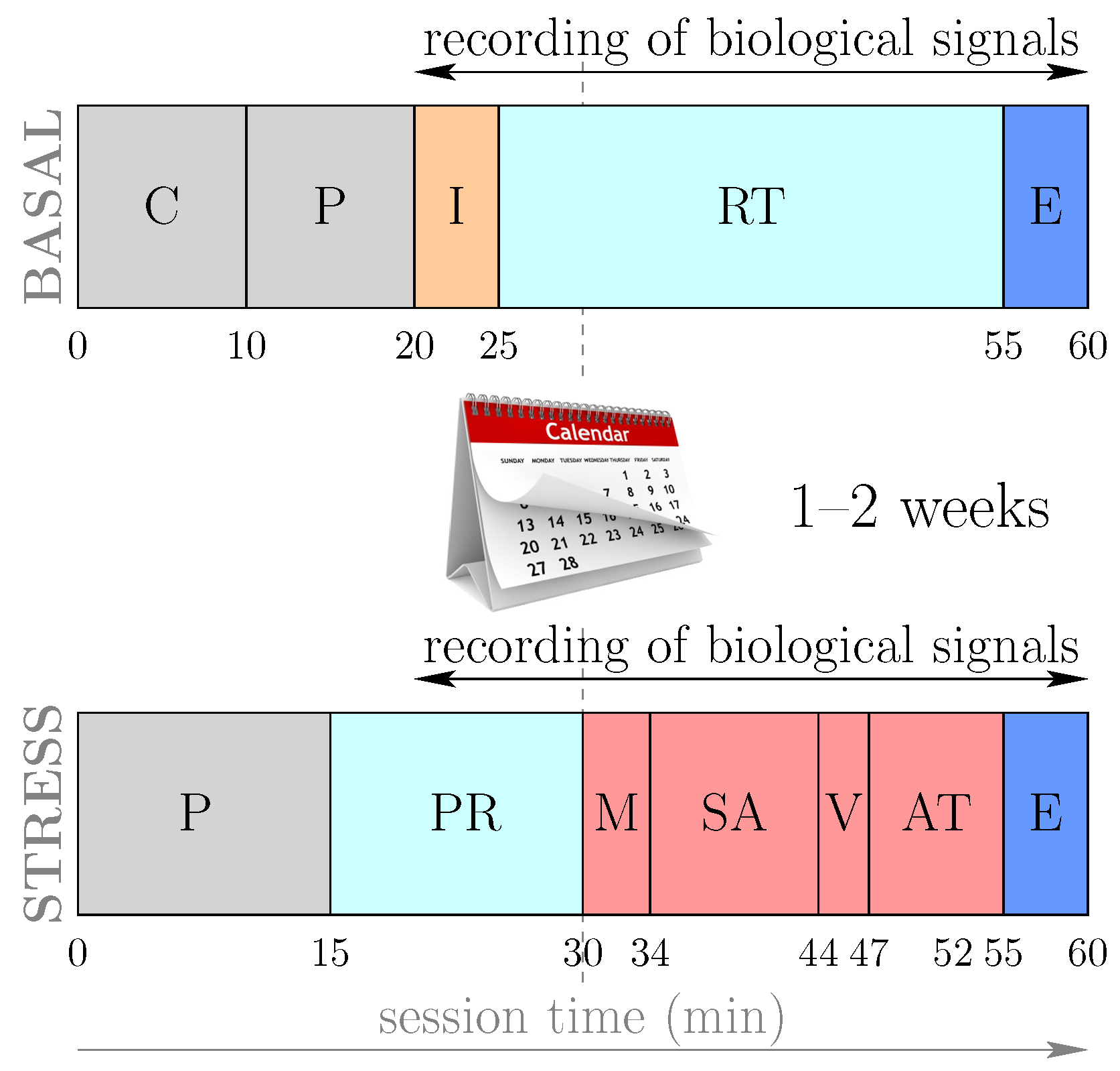
The signals were compiled in two sessions, of approximately 60 min each, undertaken simultaneously but separated by two weeks [12]. In the first session, called the basal level, the biological signals were captured; in our case, the interest is focused exclusively on the PPG signal under uninterrupted relaxation conditions. During the baseline session, the subjects were relaxed in the supine position and the physiological baseline values of each individual were established in the absence of exposure to stressors. In a second session, two weeks later, the same subjects were subjected to acute emotional stress through a memory test, a stress anticipation test, public exposure to a video and an arithmetic task, following the guidelines defined in the Trier Social Stress Test (TSST) [44]. The Trier Social Stress Test Guidelines have become a standard protocol for inducing and estimating moderate psychosocial stress in controlled settings. Many studies have confirmed its potential to induce significant changes in physiological parameters.

At the beginning of the stress level session, each subject is subjected to a relaxation period to avoid the influence of the state with which they arrive at the session. Subsequently, the following stimuli or stressors were applied consecutively: a videotaped memory test, a period in anticipation of the stress in which the patient was the informed subject—we were “evaluating their results”—the presentation of the video to an audience and finally an arithmetic task. The timing of the activities contemplated in the basal and stress level sessions is summarized in Figure 1.

From each PPG signal, 150 segments of 4 s duration (∼ten total minutes) randomly chose to have enough temporal traces of the signal that cover the dynamic spectrum captured during the sessions. With all the information collected, it is feasible to record the blood microcirculation of each individual, a faithful reflection of the exclusive peripheral capillary network of each subject. Apart from preliminary preprocessing, to alleviate the impact of the noise that the data-acquisition process entails, the PPG signals undergo a subsequent and crucial transformation that characterizes their diffusive behavior.

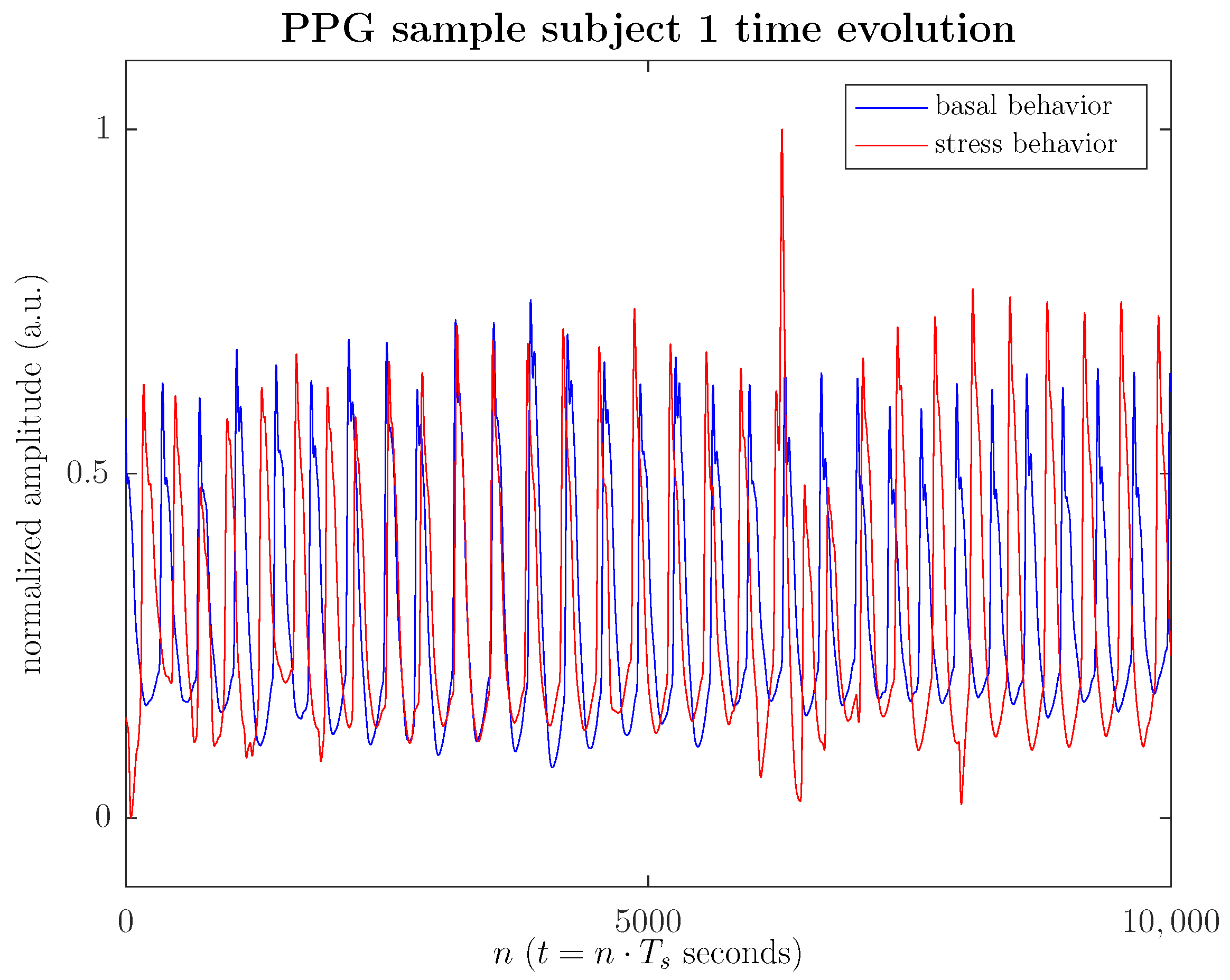
Figure 2 illustrates the time evolution of the PPG signal both in the basal and stressed states, specifically in this illustrative example, 40 s of PPG signal during a memory task after viewing a video. Figure 2 shows how the harmonic cadence of the time evolution of the PPG signal, characteristic of a relaxed state, is disrupted in the stressed state. During the stress episode, the PPG cycles undergo a more intense amplitude modulation by more accelerated breathing, which simultaneously induces a frequency modulation, translating into an increased heart rate. In any case, the PPG signal’s morphology, as seen in the figure, is frequently disturbed due to measurement noise or various artifacts (sharp peaks in the cycles), which in a morphological analysis would introduce a significant bias in the statistics considered. Furthermore, a substantial data sample is required to stabilize the morphological statistics to mitigate the spurious effects of noise or artifacts, making it difficult to use in real-time applications.

The two-dimensional $(p,q)$-planes, established via the 0–1 test, determine the geometric distribution of the diffusive behavior of the PPG signal and, therefore, become pattern-specific dynamics of each individual (cf. [45] for a more detailed description of the mathematical apparatus underlying the $(p,q)$-planes). Our CNN model’s practical recognition of these patterns constitutes the cornerstone of this work.

For that reason, the $(p,q)$-planes representative of each individual, genuine biometric pattern, as demonstrated in de Pedro-Carracedo et al. [43], serve as input to the CNN for its proper training and validation. From each individual, 150 $(p,q)$-planes were obtained in the basal state and 150 $(p,q)$-planes in the stressed state. Considering the 40 study participants, there are 12,000 dynamic patterns saved as RGB images, with dimensions initially $875\times 656$. The image was resized using the bilinear interpolation method to dimensions $224\times 168$ for their treatment by our proposal. The preprocessing of the images also required a scaling transform of the 8-bit RGB images by dividing them by 255 to rescale them from their original range $[0,255]$ to range $[0,1]$ before feeding to the proposed CNN. All the software development of the model was carried out in Python, with the assistance, among others, of Tensorflow—a framework specifically designed to facilitate the programming of the handling of NN and the previous preprocessing of the input images—and scikit-learn, a library for Machine Learning (ML).

2.2. Neural Network Architecture

Once the dataset, the 12,000 $(p,q)$-planes or representative patterns of the 40 subjects, is available, the repository is organized into two subsets of data: one for training ($\mathrm{training}+\mathrm{validation}$) and one for testing for the creation and evaluation of the model to be developed, as is usual in ML. On the first subset, the data for training is reserved for applying the DL algorithm and, thus, can obtain the model’s parameters. The data for validation is used to readjust the hyperparameters prior to each iteration of the training phase and to evaluate our model in each epoch, saving the best of them, which in our case uses a batch size of 30 patterns chosen at random if the performance finally achieved is to be achieved. The model is trained using the training set and evaluated once each epoch using the validation set. We define our training schedule to stop the training after a predefined number of epochs without improvement in validation set loss and accuracy. This can result in a final classification that falsely favors the selected validation subset and prevents the model from correctly generalizing. To accurately assess how well the model performs, it is necessary to use a separate set of data called “testing”, not included in the training phase.

Although various validation techniques organize the data in multiple ways [46], in our case, 60% of the data is assigned to the training phase, 20% to the validation phase and 20% to the test phase, according to a balancing of the data; that is, in each of the phases the same number of patterns is available in the basal and stressed state, as well as the same number of patterns for each subject.

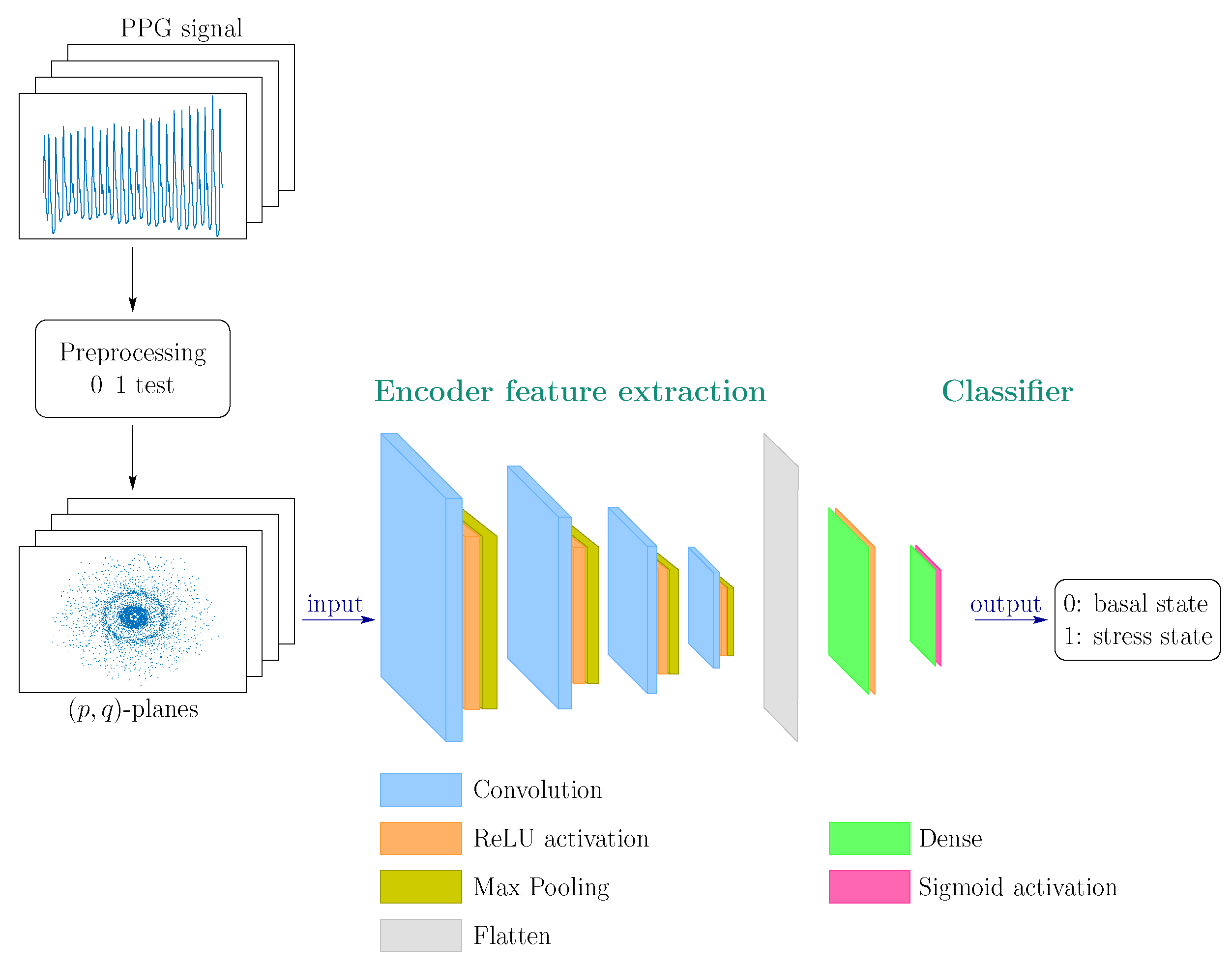
A model test design was carried out using the adapted CRISP-DM methodology. This task consisted of generating and evaluating successive models with different convolutional layers (from 2 to 4) and other numbers and sizes of initial filters, allowing us to converge on the final model with the best performance presented. The general architecture of the CNN model is illustrated in Figure 3. Since the problem of identifying a stressed state is not simple, the following successive layers are contemplated:

• Four stages of 2D convolutional layer (Conv2D) + Max Pooling 2D layer. Convolutional layers are applied to feature maps (feature maps) that are fed from RGB images of dimensions $224\times 168$ with a depth of 1 (channels). The image format is irrelevant in geometric analysis, as in our case.
  In the first two stages, the convolutional layers contain a particularly large kernel, of dimension $13\times 13$ (the filter consists of the kernel and a bias) and a pooling of $2\times 2$ (the sliding window that scrolls through the convolutional layer to output the maximum number of values from the four input window pixels). In the last two stages, the convolutional layers, with dimensions $9\times 9$ and the pooling layers, with a pooling window of dimension $2\times 2$. The kernels of dimensions $13\times 13$ facilitate the identification of those more global patterns or characteristics present in the input images while the kernels of the innermost layers, with dimensions $9\times 9$, allow more local patterns to be captured.
• Flatten Layer: a layer that transforms the input image matrix into a one-dimensional array.
• Dense Layer: fully connected hidden layer of 12 neurons with ReLU activation function. The Rectified Linear Unit (ReLU) function defined as $f\left(x\right)=x$ if $x⩽0$ and $f\left(x\right)=0$ if $x<0$, applied to the feature maps, provides the non-linearity required to carry out the task detection of stress patterns [47]. Furthermore, it has been chosen for its low computational cost to achieve good stochastic gradient descent convergence performance. It allows the network-learning process to be faster without penalizing generalization, avoiding the vanishing gradient problem that other activation functions tend to (sigmoid, tangh and others). Also, added to the dense layer, it reduces the risk of overfitting [48].
• Dense Layer: fully connected layer (fully connected) of 1 neuron with activation function sigmoid that encodes the probability that one of the two classes (basal and stress) is being treated.

Table 1. Proposed CNN architecture for stress detection/prediction.

Layer Type	Output Format	Parameters	Number of Parameters
Input	$(224,168,1)$	—	—
Conv2D	$(224,168,16)$	$\mathrm{kernel}=13,\mathrm{activation}=\mathrm{ReLU}$	2720
Max Pooling 2D	$(112,84,16)$	$\mathrm{Pool}=2$	0
Conv2D	$(112,84,16)$	$\mathrm{kernel}=13,\mathrm{activation}=\mathrm{ReLU}$	43,280
Max Pooling 2D	$(56,42,16)$	$\mathrm{Pool}=2$	0
Conv2D	$(56,42,32)$	$\mathrm{kernel}=9,\mathrm{activation}=\mathrm{ReLU}$	41,504
Max Pooling 2D	$(28,21,32)$	$\mathrm{Pool}=2$	0
Conv2D	$(28,21,32)$	$\mathrm{kernel}=9,\mathrm{activation}=\mathrm{ReLU}$	82,976
Max Pooling 2D	$(14,10,32)$	$\mathrm{Pool}=2$	0
Flatten	$\left(4480\right)$	—	0
Fully Connected	$\left(12\right)$	$\mathrm{activation}=\mathrm{ReLU}$	53,772
Fully Connected	$\left(1\right)$	$\mathrm{activation}=\mathrm{Sigmoid}$	13

describes each layer in more detail. As seen in Table 1, the number of feature maps obtained by the convolutional layers (depth or third dimension of the vector that appears in the Output Format column) increases progressively from 16 to 32. Layers of type pooling, with a pool of 2, halve the dimensions of the feature maps of the preceding convolutional layer and, therefore, their size by 4. Finally, the total number of trainable parameters is 224,265 (the sum of the values appearing in the last column).

2.2.1. Model Configuration

A critical factor in the generation of the model is the training method, which consists of the selection of the loss or cost function and the optimizer. The loss function stipulates the error between the obtained and expected outputs according to the input data of the training phase. The loss function, strongly dependent on the problem in question, must be compatible with the activation function. Given that in our particular case, we are dealing with a binary classification problem (stress or no stress), with an activation function sigmoid, the function of the loss finally chosen is the binary cross-entropy (binary cross-entropy).

The optimizer adjusts the model’s parameters by propagating the prediction error the loss or cost function offers backward. The algorithm behind the optimizer gives rise to different types of optimizers. They all constitute adaptations or improvements in the classical Stochastic Gradient Descent (SGD) algorithm. In our particular case, the optimizer that has provided the best results has been the Adaptative Moment Estimation Adam optimizer [49], which can be considered a combination of the optimizers of ADADELTA [50] and RMSProp [51], characterized due to its excellent computational efficiency and its minimal memory requirements [49]. Adam is an optimizer with adaptive moments that avoid local minima during learning. To do this, it takes as a solution not the previous gradient but the moving averages of the first and second moments of the gradient to adjust the effective learning rate to the training dynamically.

The performance of the training is subordinated to the optimizer’s operation, which, in turn, depends on the hyperparameters to which it is subjected. In this sense, considering that one of the essential metrics that govern the training and test processes is the precision (accuracy)—the value in the interval $[0,1]$ that specifies the percentage of images correctly classified—, the learning rate (learning rate) was set to 0.0001. This is one of the significant advantages of Adam, its adaptability, which allows it to gradually adjust learning to training based on the value of the learning rate hyperparameter initially established and whose stability strongly depends on the batch size [52].

2.2.2. Model Training

Once the model is defined and configured, we proceed with the training of the CNN to gradually adjust the parameters of the network layers. The training data coincides with the experiment subjects’ $(p,q)$-planes. The feature maps, duly normalized and resized, correspond to the basal state (no stress) and the stressed state, according to the previously mentioned proportions.

The set of $(p,q)$-planes of each sample in each iteration or epoch of the training algorithm is fixed by the batch size, which for this work was set at 30 to achieve the best possible performance and the correct adaptability of the Adam optimizer. The optimizer uses the number of iterations (epochs) to adjust the model parameters. The performance of the model is contingent on its value. A very high number increases the precision of the model but can also cause overfitting problems (overfitting), apart from excessive consumption of computational time in the training phase. Overfitting or overtraining causes a lack of generalization; the system “memorizes” the training data and cannot generalize the problem resolution to new data. For this work, the number of epochs equal to 100 was determined.

Overfitting happens when a model becomes too focused on the labeled training observations, which can lead to inaccurate predictions when using test data. In sum, the model learns the characteristics of the training data so literally, including defects or noise, that it cannot adequately generalize the abstract configurations. The model is limited to identifying only the pre-established conceptual details during the learning period. On the other hand, the opposite effect of overfitting can manifest itself, called underfitting, a model generalization problem caused by the scarcity of training data. Like overfitting, underfitting results in poor model performance with new samples because the model has not been trained with enough training data and does not have enough relevant patterns to provide comprehensive generalization.

Given the frequent appearance of overfitting during the modeling process of the CNN network, we focus our attention on this matter. No overfitting problems arose in the proposed model, so it was not necessary to use existing techniques for their resolution [46]. Still, they were applied during the modeling process to intermediate models, mainly by adding a penultimate layer Dropout. On the other hand, the actions carried out to prevent the appearance of overfitting were the following: (1) select the minimum number of samples to train, validate and test the model, taking into account that the dataset is not large: 60% for training, 20% for validation and 20% for testing; (2) distribute in a balanced way the number of $(p,q)$-planes of each individual in the different categories, stress and non-stress; (3) avoid the excess of epochs with the “early stop” technique of the training through the use of callbacks that allow training to be stopped before overfitting occurs during the 100 epochs established for training as well as storing the best model obtained.

2.3. Evaluation Metrics

The training, validation and testing phases of any DL or ML model require textual or visual tools that allow monitoring of its evolution. In this way, it is easier to interpret potential problems that may arise during model fitting and finally certify the goodness of fit of the proposed model. The metrics widely used to assess binary classification model performance are described below.

2.3.1. Confusion Matrix

The confusion matrix [53] is not properly a metric to estimate the performance of a classification in ML. However, it does bring together the factors used in the performance metrics used in this work. In a stress classification and detection problem, as is the case at hand, the aim is to identify, based on an input $(p,q)$-plane, whether or not an individual is stressed. The variable that identifies the status or class of a subject is called the objective variable. If the individual is stressed, the target variable is assigned a value of ‘1’; otherwise, it is assigned a value of ‘0’. The confusion matrix contains a two-dimensional table, as reflected in

Table 2. Confusion matrix scheme.

		Actual
		Positive	Negative
Predicted	Positive	True Positive (TP)	False Positive (FP)
	Negative	False Negative (FN)	True Negative (TN)

. In its columns, the classes are labeled according to the current state according to the actual training data. Its rows represent the states predicted after the application of the model once trained and validated.

The terminology associated with the confusion matrix is as follows:

• True positives (True positives or TP): number of samples whose true and predicted class is ‘1’.
• True negatives (True negatives or TN): number of samples whose true and predicted class is ‘0’.
• False positives (False positives or FP): number of samples whose real class is ‘0’ and the predicted class is ‘1’.
• False negatives (False negatives or FN): number of samples whose real class is ‘1’ and the predicted class is ‘0’.

Ideally, there are always correct predictions, with no FPs or FNs.

2.3.2. Accuracy

The accuracy metric is formulated as

$$\mathrm{Accuracy}=\frac{\mathrm{TP}+\mathrm{TN}}{\mathrm{TP}+\mathrm{FP}+\mathrm{TN}+\mathrm{FN}}.$$

(1)

With this metric, as reflected in Equation (1), the total number of samples correctly classified by the model (for both classes) is obtained concerning the total number of all classified and predicted samples.

2.3.3. Precision

The metric precision is defined as

$$\mathrm{Precision}=\frac{\mathrm{TP}}{\mathrm{TP}+\mathrm{FP}}.$$

(2)

This metric represents, according to Equation (2), the proportion of samples correctly classified as positive (samples with stress or TP) of the total samples classified and predicted as positive ($\mathrm{TP}+\mathrm{FP}$). Therefore, this metric quantifies the classifier’s performance concerning false positives. In order to minimize FPs, precision should be close to 1.

2.3.4. Recall

The recall metric is

$$\mathrm{Recall}=\frac{\mathrm{TP}}{\mathrm{TP}+\mathrm{FN}}.$$

(3)

This metric establishes, according to Equation (3), the proportion of samples correctly classified by the model as positive (TP) compared to the total number of positive samples ($\mathrm{TP}+\mathrm{FN}$). Therefore, this metric quantifies the classifier’s performance concerning failed predictions. The sensitivity should be close to 1 to minimize FNs.

Sensitivity and precision take values in the range $[0,1]$. The model will behave more efficiently as the metrics tend to 1, although an increase in one of them necessarily entails a decrease in the other.

2.3.5. $F_1$-Score

The metric $F_1$-score is the harmonic mean of the sensitivity and precision, as in Equation (4).

$$F_1-\mathrm{score}=2·\frac{\mathrm{precision}·\mathrm{recall}}{\mathrm{precision}+\mathrm{recall}}.$$

(4)

When sensitivity and precision are disparate, the metric $F_1$-score tends to a smaller value. Therefore, the model will perform better the closer $F_1$-score is to 1.

2.3.6. Cohen’s Kappa Coefficient

Cohen’s kappa coefficient $\kappa$, whose value is $[-1,1]$, uses the confusion matrix. Unlike the accuracy metric, this coefficient considers the distributions of the actual and predicted classes. When the model’s precision degrades due to the imbalance in said distributions, the kappa coefficient admits a more objective interpretation of the model’s performance, preferentially attending to the minority class [54]. So,

$$\kappa =\frac{p_0-p_e}{1-p_e},$$

(5)

where $p_0$ represents the accuracy of the model and $p_e$ is a measure of the agreement between the model predictions and the values of the actual classes (labels). In a specific context of binary classification, as in our work, this measure amounts to $p_e=p_{e_1}+p_{e_2}$, where $p_{e_i}$ is obtained by multiplying the percentage of the predicted class by the percentage of the actual class, assuming they are independent: $p_e=p_{e_1,\mathrm{real}}·p_{e_1,\mathrm{pred}}+p_{e_2,\mathrm{real}}·p_{e_2,\mathrm{pred}}$.

According to Equation (5), the further the distributions are from the predicted and actual classes, the smaller the value of the coefficient $\kappa$ maximum achievable. The maximum value of $\kappa$ poses a limiting scenario in which the number of false negatives and false positives in the confusion matrix is zero; all observations are correctly predicted. The coefficient $\kappa$ reaches its maximum value when the model operates with balanced data, as is the case at hand. The numerator of Equation (5) denotes the difference between the overall precision of the model and the overall precision achieved by chance; the denominator describes the maximum value of the difference of the numerator. An admissible model will have a maximum and observed difference close to each other, leading to a null value of $\kappa$. In a random model, the overall precision is random and the numerator vanishes, resulting in a value of $\kappa$ equal to 0. The value of $\kappa$ can assume negative values when the general precision of the model is even lower than that which can be set at random.

Jacob Cohen suggested an interpretation of the degree of agreement according to the value of the coefficient $\kappa$, which was later adapted by Mary L. McHugh [55], as illustrated in

Table 3. Level of agreement according to the $\kappa$ coefficient.

Range of Values of $\mathit{\kappa }$ Coefficient	Matching (Level of Agreement)
$[0.00,0.20]$	none
$[0.21,0.39]$	minimal
$[0.40,0.59]$	weak
$[0.60,0.79]$	moderate
$[0.80,0.90]$	strong
$[0.91,1.00]$	almost perfect

. In short, the coefficient $\kappa$ is a measure of the efficiency of the model as opposed to a classifier that behaves randomly. Somehow, it intends to correct the evaluation bias by considering a correct classification by chance. Although the coefficient $\kappa$ has become a frequently used metric to compare classifiers, its behavior makes it difficult to interpret the values obtained. A heated debate has arisen about the advisability of its use as a performance metric or a model, which is why some authors advise against its use to compare different classifiers [56].

2.3.7. Mathews Correlation Coefficient

The Mathews MCC correlation coefficient also comes from the categories or classes of the confusion matrix. Given that it is a particular case of the Pearson correlation coefficient, it allows quantifying the existing correlation between the real classes (TP and TN) and the classes predicted (FP and FN).

$$\mathrm{MCC}=\frac{(\mathrm{TP}·\mathrm{TN})-(\mathrm{FP}·\mathrm{FN})}{\sqrt{(\mathrm{TP}+\mathrm{FP})·(\mathrm{TP}+\mathrm{FN})·(\mathrm{TN}+\mathrm{FP})·(\mathrm{TN}+\mathrm{FN})}}.$$

(6)

The value of the Mathews correlation coefficient, according to Equation (6), is within the range $[-1,1]$, where $-1$ indicates a complete misclassification, while $+1$ indicates a perfect classification. A null value refers to a random prediction. MCC is especially interesting because it takes a high value only if the prediction performed well in all categories of the confusion matrix (TP, TN, FP and FN) in proportion to both the size of the positive samples and the size of the negative samples of the dataset in question [57]. It is also very helpful in scenarios with unbalanced classes. Contrary to other metrics, such as accuracy, precision, recall or $F_1$-score, MCC recognizes the inadequacy of the model with respect to predicting instances, reflecting its real predictive power correctly.

2.3.8. Precision–Recall Curve

The Precision–Recall (PR) curve plots the sensitivity rate (true positives) on the abscissa and the precision metric on the ordinate (positive values correctly predicted) for different probability thresholds. The area under the PR curve, called PR AUC (Area Under Curve), allows evaluating the performance of the classifier in terms of balance between precision and recall. Inspecting the AUC is advisable when the samples are not balanced, that is, when there are few samples of a positive class. This assumption is not the case for the dataset available in this work since the number of positive samples coincides with the number of negative samples. The greater the area under the curve, the greater the model’s performance. In other words, the optimum would be a curve as close as possible to the upper right corner (high recall and high precision).

2.3.9. ROC Curve

The ROC (Receiver Operation Characteristics) curve plots the false positive rate on the abscissa and the recall rate on the ordinate. The ROC curve relates the sensitivity of the model (recall) to the number of negative samples classified as positive (optimistic failures). An increase in recall (higher rate of positives predicted by the model compared to the total number of real positives) implies fewer false negatives and, therefore, more false positives, in short, a more optimistic model. The closer the ROC curve is to the upper left corner of the graph, the better the model performs. However, it must be underlined that when the data are unbalanced, with few positive samples, the ROC curve, or the value of the area of the ROC curve (ROC AUC), can be misleading, with a plot very close to the ideal but with too low a precision. In this sense, the relevance of the ROC curve is limited to contexts with balanced data or situations in which optimistic failures are intended to be highlighted. The PR curve would be more informative in the presence of unbalanced data.

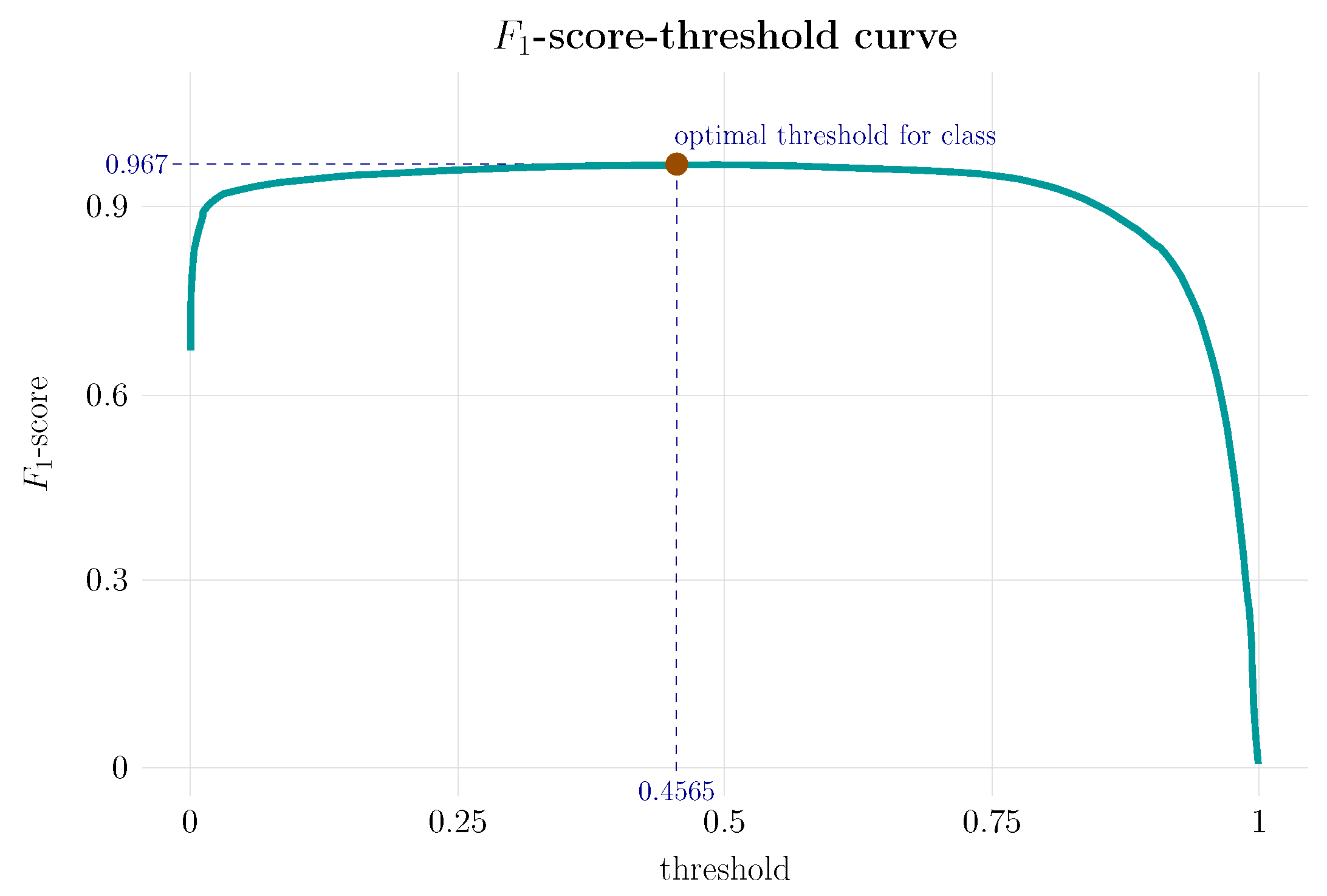
2.3.10. Curve $F_1$-Score-Threshold

This curve represents the $F_1$-score metric for different threshold values. $F_1$-score-Threshold complements the information provided by the PR curve considering jointly the values of the precision and recall measures, compacted in their harmonic mean. It allows the evaluation of the stability of the system performance for different threshold values. In a high-performance, stable system, the curve is nearly a straight line; the value of $F_1$-score remains approximately constant and close to 1 for the full range of possible threshold values.

3. Results

Before weighing the yields achieved and comparing them with other approaches published in the scientific literature, it is worth examining the entire process that has led to the CNN model presented in this paper.

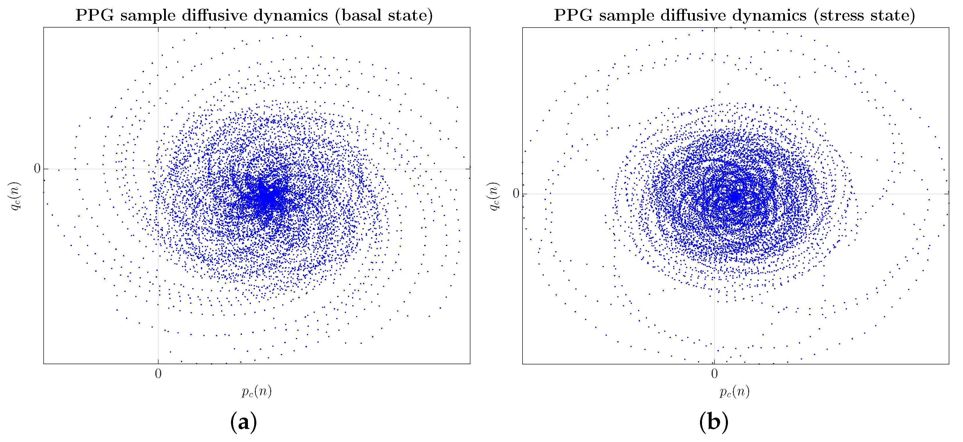
First, as an example of preprocessing data, Figure 4 shows two input $(p,q)$-planes, one from the basal state, as shown in Figure 4a, and the other from the stress state on the same subject, as illustrated in Figure 4b.

Considering the $(p,q)$-planes, a more regular spiral configuration can be seen in the case of the user in the basal state, mainly in the central bulb, as shown in Figure 4a. In a stressed state, the geometric structure experiences a greater spatial dispersion both in the arms of the spiral and in the central bulb, which adopts a more ellipsoidal arrangement, blurring the regular configuration, as reflected in Figure 4b. In any case, in the absence of a more exhaustive study of the geometric structures exhibited by the $(p,q)$-planes and their functional link with the physiological system that generates the PPG signal, we believe that the mechanism behind the blurring of the configuration regular in a kind of multifractal tessellation is related to a dynamic tending towards chaos.

In more physiological terms, it leads to a more flexible and adaptable physiological disposition to quickly counteract the stress response and restore the homeostatic balance of the organism as soon as possible. In this regard, applying a convolutional network model has been pivotal in detecting an individual’s basal or stress state. The successive convolutional layers of the network learn a hierarchy of invariant features in the $(p,q)$-planes, unique to each individual and indiscernible to the human eye. An in-depth analysis of the maps obtained by the different layers of the model’s feature extractor would provide relevant information on these factors common to all individuals to further advance the study and classification of stress at its different levels.

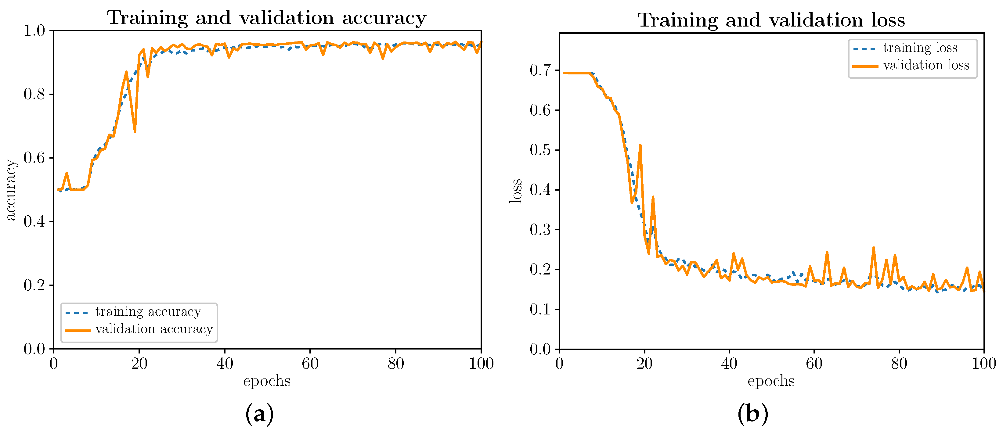
Next, let us begin by evaluating the training and validation process illustrated in Figure 5a,b, respectively, for the 100 iterations (epochs) established by design. As can be seen, the training and validation processes behave similarly. In the first few iterations, as Figure 5a shows, until around iteration 16, you do not notice an increase in precision, as you would ideally expect. During the first iterations, the precision fluctuates and then quickly scales up to a value close to 100% (∼97%), remaining around 97% from iteration 40 onwards. The loss function, as illustrated in Figure 5b, remains virtually stable around 0.7 because, not without some logic, learning is hard and slow in the first bars. Subsequently, the loss function decreases sharply until iteration 40, slowly decreasing until it reaches a value close to 0 (∼0.13). Optimizing the gradient descent algorithm keeps significant parallelism between the training and validation data. This conformance in the training and validation data behavior is due to the Dropout layer introduced at the end of the convolutional network. The Dropout layer avoids the slight overfitting that comes with a somewhat more complex model than is strictly necessary.

The trained model, after overfitting is removed, consists of four convolutional layers with kernel of $13\times 13$, $13\times 13$, $9\times 9$ and $9\times 9$, respectively and associated Max Pooling layer of $2\times 2$ (for the four layers), Flatten layer and Dense layer of 12 neurons (batch size of 30 and number of epochs equals 100) and the optimizer Adam.

3.1. Metric Results

The results that emerge from the evaluation metrics are detailed below.

3.1.1. Model Confusion Matrix

An analysis of the model’s accuracy and loss function is indispensable in terms of model performance. A ∼96.7% accuracy was achieved with the test data. These data imply a high percentage of success in the classification with data not known a priori by the model. However, suppose it is intended to delve into the model’s behavior in more detail. In that case, it is convenient to pay attention to other evaluation metrics that contemplate how many samples among those labeled as the basal state have been classified correctly (NT) or incorrectly (FP) or, similarly, how many samples among those labeled as a stressed state have been classified correctly (TP) or incorrectly (FN). 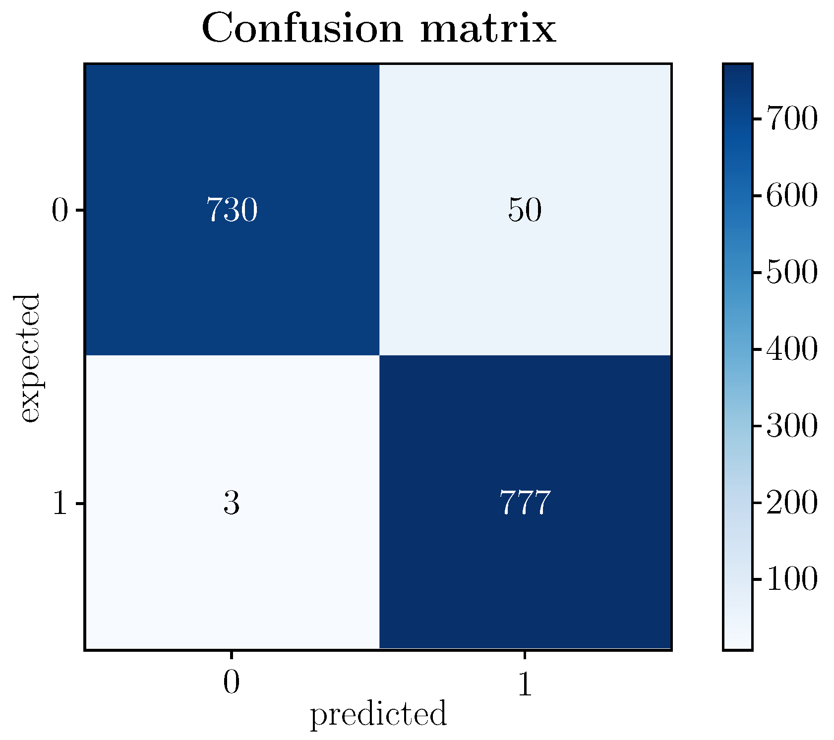Figure 6 shows the confusion matrix of the proposed model.

Of the 1560 test images (testing) corresponding to the 40 participants in the experimental protocol, 780 concern subjects in a basal state and 780 individuals in a stressed state. According to Figure 6, the model correctly detects 730 as TN (baseline state) and 777 as TP (stressed state), which means that the model correctly predicts a high rate of samples labeled as baseline or stressed.

The fact that the model presents a very high TP value (777 out of 780) and, consequently, a very low FP value (3 out of 780) is especially revealing since the purpose of the model is precisely the detection of a stressed state in order to prevent potential pathologies that could lead to severe health disorders. In the case of the value of TN, although it remains at high levels (730 of 780), it is lower than that of TP, implying that the FN value is somewhat higher than FP (50 of 780). Whatever its incidence, without detracting from it, since it is still a prediction error of the model, it is less relevant in terms of the expected goal. In any case, there are various metrics that, based on the confusion matrix, exploit the relationships established between the categories of the matrix. These links highlight aspects of the model that complete its analysis and the quality attributed to it, as detailed below.

Concerning the sensitivity (recall)—the proportion of correct predictions of each class for the total observations of the said class—, its increase runs inextricably to the detriment of precision (accuracy) and vice versa. Therefore, for the stressed state class, it adopts a very high value (∼1), while for the basal state class, its value remains high but somewhat less (0.94). Sensitivity is key in this work because it quantifies the model’s performance against failed predictions. In particular, the sensitivity of the proposed model is practically 1, indicating that there are hardly any failures in the predictions of the stressed state. Therefore, a stress episode can be prevented and contained in almost all obvious cases before the situation worsens.

In the context of the problem posed in this paper, $F_1$-score, a metric that is subject to FP and FN, that is, to sensitivity and precision, does not provide relevant information, since both Error types are balanced. However, sensitivity is given greater significance than precision in the case of the positive class, the stressed state. It is preferable to optimize the value of sensitivity rather than precision, which entails minimizing FN to detect the detrimental effects of stress as far as possible. As the data are balanced, the metric is of no great interest, especially when its value for the basal state and stressed state classes is very high, ∼0.96 and ∼0.97, respectively, thus confirming the model’s goodness.

Cohen’s kappa coefficient presumes to be more notorious than accuracy when faced with unbalanced data, contrary to what happens in our work. However, it always helps to corroborate the model’s reliability with its estimation. In addition, the similar distributions of the categories of the confusion matrix facilitate the interpretation of the kappa coefficient $\kappa$, whose value is very high, ∼0.93, which, according to Jacob Cohen and Mary L. McHugh [55] (see Table 3), is equivalent to an almost perfect agreement between the actual classes and the predicted classes. This consistency provides a very high measure of the number of model predictions that cannot be explained by chance.

The Matthews correlation coefficient further confirms the real capacity of the model to predict instances correctly. An almost perfect classification is available with a value close to 1, ∼0.93. The prediction remained at ideal levels in all the categories of the confusion matrix (TP, TN, FP and FN) by the balance of positive and negative samples of the dataset of $(p,q)$-planes with which it was operated. Cohen’s kappa and Matthews’ correlation coefficients did not reach the ideal goal 1.

3.1.2. ROC, PR and $F_1$-Score-Threshold Curves

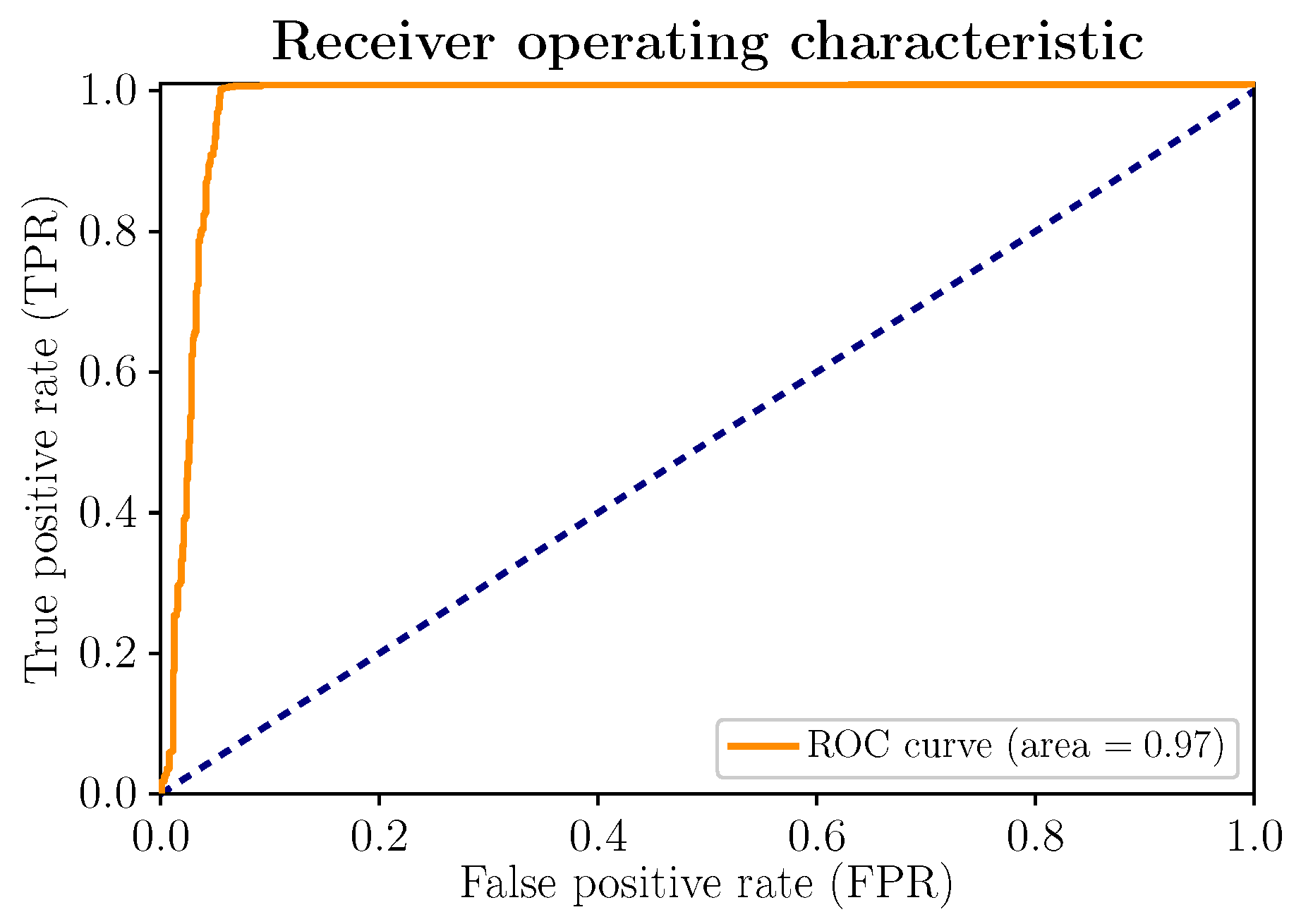
Figure 7 shows the ROC curve of the model. Its layout is scrupulously close to the upper left corner. Therefore, an increase in sensitivity does not necessarily imply the appearance of more false positives (FPs) and, consequently, does not affect the excellent performance of the model, summarized in the area under the curve ($\mathrm{ROC}\mathrm{AUC}=0.97$), very close to 1.

With unbalanced data, which is not the case in the present work, if there are few positive samples, the value of the ROC curve, as well as the area under the curve ($\mathrm{ROC}\mathrm{AUC}$), could present high values; the FP rate (number of false positives/number of negative samples) tends to remain low due to the large number of negative observations, which makes its informative function less relevant by not reflecting the true performance of the classifier. In this regard, the PR curve, analyzed below, becomes a complementary indicator. However, for balanced data, as is the case at hand, the ROC curve and the area under the curve ($\mathrm{ROC}\mathrm{AUC}$) are appropriate indicators. For the rest, the ROC curve clearly illustrates the relationship that is established with the false positives. As already advanced with the confusion matrix, they are counted more significantly than the false negatives: 50 of 780 for FP, compared to 3 of 780 for FN.

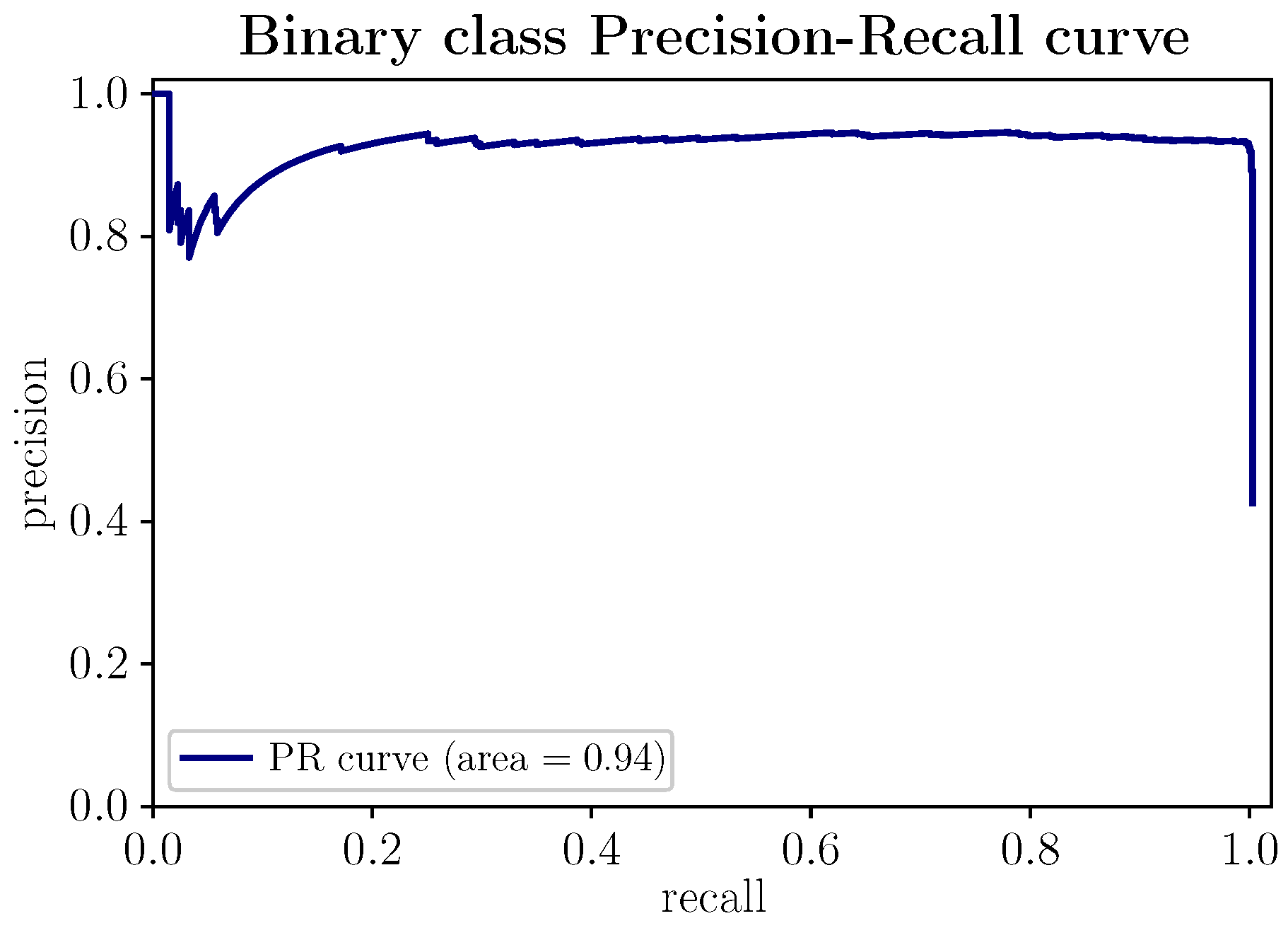
In Figure 8, the Precision–Recall curve of the proposed model is represented. This curve shows the relationship between the metrics precision and recall. The more the curve trace extends towards the upper right corner, reflected in the trend to 1 of the area under the curve $\mathrm{PR}\mathrm{AUC}$ (∼0.94), the better the model performance. The PR curve makes it possible to determine from what value of precision recall degrades and vice versa. The PR curve suggests the most significant number of positive samples (stressed state) the model can predict in scenarios with balanced data. In the presence of unbalanced data, with few positive samples, the PR curve would deviate from its optimal regime, making it a representative precision indicator, given the low probability of the positive class.

Finally, the $F_1$-score-Threshold curve, shown in Figure 9, completes the information provided by the ROC curve and the area under the curve $\mathrm{ROC}\mathrm{AUC}$ since it integrates with $F_1$-score the precision and sensitivity. In Figure 9, the stability and performance of the model can be clearly appreciated. For a wide range of threshold values, the value of $F_1$-score remains constant at a height of practically 1, with a maximum value of ∼0.97 for a threshold of $0.4565$ of the positive classes.

4. Discussion

In stress detection using machine-learning techniques, the most significant performance is obtained when physiological markers from heart rate are used together, temperature, humidity, blood pressure and vocal timbre [58,59]. In such a competitive job market, overwork has become a handicap that is difficult to overcome, resulting in reduced performance in professional activity. In many cases, self-imposed social pressure is also felt in the academic field, with increasingly unbridled levels of demand or in activities as routine as driving a vehicle, in which precisely a lack of concentration, the result of fatigue, can lead to a fatal outcome [60]. Therefore, early detection of stress not only helps to prevent accidents or severe morbid disorders but also to consolidate healthier work or study climates.

Although the evaluation of stressful situations was traditionally limited to highly controlled environments, with the technological development of peripheral devices, stress detection is undertaken in real-time through portable devices, such as a bracelet, a watch or the mobile phone itself, even very low-cost home-made devices. The growth experienced by sensor technology has been transferred to the ubiquitous universe of mobile devices. Today, multiple physiological parameters, such as, e.g., nasal skin temperature, heart rate, eyelid movement, voice inflection and typing, can be captured through the different interfaces or sensory extensions that portable devices consist of without altering the behavioral routine. In any case, the performance exhibited by real-time stress-detection techniques is still somewhat relevant compared to traditional methods practiced in controlled environments [61].

The most common classification algorithms that support learning algorithms in the process of detecting mental stress are circumscribed to logistic regression, KNN (K-Nearest Neighbor), RF (Random Forest) and SVM (Support Vector Machine). For the validation of classification models, cross-validation k-fold ($k=5$ or $k=10$) and cross-validation leaving one subject out (leave-one-out cross-validation) [59]. Of all physiological indicators, ECG-derived signals such as heart rate and skin conductance (GSR) provide the highest performance in terms of accuracy. However, it is necessary to extract many variables to place the performance at acceptable levels, which are often insignificant. In any case, with the number of variables, the computation time also increases, which jeopardizes its application potential in real-time environments. The characteristics usually provided to classification models attend to linear aspects, both in the time domain and frequency domain and to non-linear aspects of biological signals [62,63,64,65].

Concerning the PPG signal, its close relationship with the cardiovascular system and its easy acquisition, even with the simple camera of a mobile [66], makes it a relevant candidate for stress detection. Previous works related to the identification of a stressful situation through the PPG signal are summarized in Table 4, in which it can be seen how the performance obtained is notorious due to the marked bias that noise induces in the morphology of the signal, as previously mentioned.

It should be noted that in all the studies that use the PPG signal, either in isolation or with other biological signals (multimodal analysis) [65], the characteristics that make their cataloging possible refer to the morphology of the signal implicitly or explicitly. As a result of this, all of them are strongly conditioned by psychophysiological variations (e.g., changes in an emotional state, physical activity), by noise disturbances coupled in the acquisition phase of the data or due to statistical inconsistencies due to the non-stationarity of the signals (time interval of the measurements) [27].

In that sense, it is worth highlighting the work of Seongsil Heo et al. [67], in which the authors propose a debugging method (denoising) of the signals PPG data in order to refine its temporal definition and thus to be able to extract higher quality features. The authors demonstrate how removing noise from the PPG signal achieves stress detection with a higher accuracy rate than other conventional approaches. In the same way, in the work of Nilava Mukherjee et al. [68], the first hardware solution is proposed that enables real-time detection of stress. However, to achieve high effectiveness, due to the susceptibility of the PPG signal morphology, the use of 60 signal characteristics is prescribed.

With these backgrounds, the solution proposed in this work is entirely new; it ultimately moves away from the usual methodology, anchored in the morphology of the PPG signal and approaches the detection of stress from the dynamic approach of the PPG signal, inspired by the stochastic nature of blood flow. A diffusive model highly dependent on the vascular bed, whose physical structure is unique to each individual, is a framework to characterize an individual’s stress level through a CNN.

According to Table 4, it can be seen how the initial attempts for stress detection assume a multimodal character in the extraction of physiological characteristics. For a more comprehensive review, we recommend consulting the works of Shruti Gedam and Sanchita Paul [59] and Giorgos Giannakakis et al. [65], apart from those specifically referred to in Table 4 and the references within them. The conjunction of various biological signals in the stress-detection process, added to the computational requirement inherent in the complexity of the feature-extraction algorithms, make it impossible to integrate a possible hardware solution that operates in real-time in a portable device [69]. With this objective, in recent years, stress-detection models have been proposed that reduce the analysis to a single biological signal from which to extract reliable stress indicators. In addition, the advanced signal-processing techniques that accompany the most modern classifiers favor optimal levels of discrimination between psychophysiological states.

Table 4. Previous work on stress detection using the PPG signal.

Previous Studies	Population (Subjects)	Biological Signals	Classifier	Best Accuracy (%)
Khalilzadeh et al. (2010) [70]	9	BVP, RR, EEG, GSR, PPG	Elman neural network	82.6
McDuff et al. (2014) [71]	10	PPG (HRV), BR	SVM	85.0
Maaoui et al. (2016) [72]	12	PPG (HRV)	SVM RBF	94.4
McDuff et al. (2016) [73]	10	PPG (HR, HRV, BR)	Naïve Bayes	86.0
Mozos et al. (2016) [74]	18	PPG, EDA, HRV	AdaBoost, KNN, SVM RBF, SVM	94.0
Giannakakis et al. (2017) [75]	23	facial rPPG, facial videos	KNN, GLR, NVB, SVM	91.68
Cheema and Singh (2019) [76]	32	PPG, ECG	LS-SVM	93.0
Kalra and Sharma (2020) [77]	15	PPG	MLPNN, DNN	91.0
Bobade and Vani (2020) [78]	15	ECG, PPG, ST, RESP, EMG, EDA, ACC	DT, RF, AB, LDA, KNN, SVM, ANN	95.0
Indikawati and Winiarti (2020) [79]	15	ST, PPG, EDA	LR, DT, RF	96.9
Bhanushali et al. (2020) [80]	15	ECG, PPG, ST, RESP, EMG, EDA	LDA, RF, SVM, ANN	98.0
Nath and Thapliya (2021) [81]	40	EDA, PPG, IBI, ST	RF	94.0
Heo et al. (2021) [67]	15	PPG	DT, AdaBoost, RF, LDA, SVM	96.5
Anwar and Zakir (2022) [82]	27	PPG (PRV)	KNN, GA	81.0
Mukherjee et al. (2022) [68]	15	PPG	AE, SVM	99.0
Paul et al. (2023) [83]	32	PPG	Threshold-based classification	98.43
Our approach (2023)	40	PPG (diffusive dynamics)	CNN	97.0

Table 4. Previous work on stress detection using the PPG signal.

Previous Studies	Population (Subjects)	Biological Signals	Classifier	Best Accuracy (%)
Khalilzadeh et al. (2010) [70]	9	BVP, RR, EEG, GSR, PPG	Elman neural network	82.6
McDuff et al. (2014) [71]	10	PPG (HRV), BR	SVM	85.0
Maaoui et al. (2016) [72]	12	PPG (HRV)	SVM RBF	94.4
McDuff et al. (2016) [73]	10	PPG (HR, HRV, BR)	Naïve Bayes	86.0
Mozos et al. (2016) [74]	18	PPG, EDA, HRV	AdaBoost, KNN, SVM RBF, SVM	94.0
Giannakakis et al. (2017) [75]	23	facial rPPG, facial videos	KNN, GLR, NVB, SVM	91.68
Cheema and Singh (2019) [76]	32	PPG, ECG	LS-SVM	93.0
Kalra and Sharma (2020) [77]	15	PPG	MLPNN, DNN	91.0
Bobade and Vani (2020) [78]	15	ECG, PPG, ST, RESP, EMG, EDA, ACC	DT, RF, AB, LDA, KNN, SVM, ANN	95.0
Indikawati and Winiarti (2020) [79]	15	ST, PPG, EDA	LR, DT, RF	96.9
Bhanushali et al. (2020) [80]	15	ECG, PPG, ST, RESP, EMG, EDA	LDA, RF, SVM, ANN	98.0
Nath and Thapliya (2021) [81]	40	EDA, PPG, IBI, ST	RF	94.0
Heo et al. (2021) [67]	15	PPG	DT, AdaBoost, RF, LDA, SVM	96.5
Anwar and Zakir (2022) [82]	27	PPG (PRV)	KNN, GA	81.0
Mukherjee et al. (2022) [68]	15	PPG	AE, SVM	99.0
Paul et al. (2023) [83]	32	PPG	Threshold-based classification	98.43
Our approach (2023)	40	PPG (diffusive dynamics)	CNN	97.0

As is known, stress is closely linked to the cardiorespiratory system, whose physiological manifestation extends in its entire spectrum throughout the entire organism, including, e.g., breathing, autonomic nervous system, skin temperature and sweating. The ECG signal is its maximum exponent; therefore, it has been used in countless works, leading to the detection of stress [59]. However, its acquisition is uncomfortable for the subject on which the electrodes required for its measurement are arranged. In this sense, the PPG signal has become a reliable alternative to the ECG signal since it is effortless to acquire, with minimally invasive techniques and it contains the same physiological information as the ECG signal [84].

Focusing on those previous works that only use the PPG signal to detect the presence of stress in a subject, with an accuracy greater than 90%, Choubeila Maaoui et al. [72] use seven extracted characteristics of the PPG signal. The pulse signal was acquired using a web camera from the facial analysis of the face. They achieve 94.4% accuracy using an SVM BRF classifier. Prerita Kalra and Vivek Sharma [77] use 18 characteristics of the PPG signal to identify a possible stress episode, 9 of them from the time domain and the remaining 9 from the frequency domain. With a DNN, they reach 91% accuracy. Seongsil Heo et al. [67] propose a stress-detection methodology based on the analysis of 26 characteristics of the PPG signal. With different classifiers, they obtain a maximum accuracy of 96.5% whenever an LDA classifier is used. In this work, unlike the previous ones, the authors demand a minimum trace of the PPG signal, in their case of 120 s, to guarantee the published performances. Nilava Mukherjee et al. [68] propose for the first time a hardware solution that makes it possible to detect stress in real time, among four possible states—baseline, stress, amusement and meditation—with an accuracy of 99%, an $F_1$-score of 99% and a sensitivity 98%. Memory requirements are not severe (∼1.7 MB) and latency time is ∼0.4 s, with a minimum PPG signal trace of 5 s. To preserve such high performance, they require the extraction of 60 characteristics of the PPG signal. Recently, Avishek Paul et al. [83] used a threshold classification method to, based on two characteristics of the PPG signal, identify a stress episode with an accuracy of 98.4%, a sensitivity of 96.87% and a specificity of 100%. However, the authors do not provide conclusive evidence on the minimum PPG signal trace, memory requirements or latency time needed to satisfy such excellent performance.

The potential of our proposal resides in the fact that with a single characteristic of the PPG signal, its diffusive dynamics, which houses the integral spectrum of cardiorespiratory factors, it is feasible to detect the stress of an individual with an accuracy and $F_1$-score of ∼97% and a sensitivity also of 97% but ∼100% for the stressed state class. Its migration to portable hardware operating in real time is immediate since its memory requirements are minimal (∼2.8 MB, of the same order of magnitude, as suggested by Nilava Mukherjee et al. [68]) and it takes 4 s of PPG signal, compared to 5 s for the latter, with a latency time of ∼19–20 ms, to detect stress with virtually 100% reliability.

5. Conclusions

In this article, we propose a binary classification model based on CNNs to detect the presence of acute stress in a subject through the PPG signal. Unlike other previous works, our model only requires a single characteristic of the PPG signal, its diffusive dynamics, a property inherent to the vascular bed of each human being, unrelated to external conditions and very stable over time except in the case of pathologies that could damage the vascular structure. Most works that use biological signals to identify stress episodes implicitly or explicitly resort to temporal or frequency characteristics subject to their morphology. Therefore, they are very vulnerable to noise in data-acquisition systems and eventual psychophysiological variations, such as physical activity or a change in an emotional state, which distort an accurate measure of stress. The PPG signal’s diffusive dynamics reflect each individual’s reactive and inalienable tendencies, less prone to exogenous and endogenous spurious disturbances that undermine the veracity of the stress diagnosis.

The solvency of the diffusive dynamics of the PPG signal in the face of external and internal instrumental artifacts makes it possible, with its single analysis, to identify episodes of acute stress with a high percentage of success with a minimum signal sample. The solution proposed in this work reaches 97% accuracy, like its $F_1$-score, with a sensitivity of 99%. With a latency time of at most 20 ms, the model requires only 4 s of PPG signal to report a stressed state. In addition, the modest memory requirements, ∼2.8 MB, make our solution a highly attractive alternative for implementation in consumer electronics (portable devices), which would allow not only early and accurate stress detection but also the expeditious deployment of the necessary countermeasures before their adverse effects have a significant impact on the family, economic and work spheres.

The CNN model has obtained a very positive evaluation in terms of the different evaluation metrics that commonly certify the validity of a model. A weak point that partly undermines its respectable credit is the FP value, 50 of 780, compared to the FN value, 3 of 780. Although the FP value is not entirely unacceptable, with a lower cost than the impact of FN, it is worth further work to refine the model, mitigate the losses subject to the depth of the CNN and minimize their degree of incidence. Along the same lines, future work should delve into the physiological mechanisms of stress and how they converge in the diffusive dynamics of the PPG signal so that the CNN model can be optimized with an efficient and systematic adjustment of the hyperparameters. Its diagnostic prospects are promising, even as a recommender system. However, its expectations will be fulfilled when it helps to detect stress sufficiently in advance, partly mitigating the serious consequences that it derives from modern society.