A Symbol Recognition System for Single-Line Diagrams Developed Using a Deep-Learning Approach

Featured Application

The present study is among the first research efforts to generate augmented datasets of complex single-line diagrams to detect symbols using deep-learning-based algorithms. The work determines the impacts of augmented datasets on model performance and indicates future directions in the field of engineering drawings.

Abstract

In numerous electrical power distribution systems and other engineering contexts, single-line diagrams (SLDs) are frequently used. The importance of digitizing these images is growing. This is primarily because better engineering practices are required in areas such as equipment maintenance, asset management, safety, and others. Processing and analyzing these drawings, however, is a difficult job. With enough annotated training data, deep neural networks perform better in many object detection applications. Based on deep-learning techniques, a dataset can be used to assess the overall quality of a visual system. Unfortunately, there are no such datasets for single-line diagrams available to the general research community. To augment real image datasets, generative adversarial networks (GANs) can be used to create a variety of more realistic training images. The goal of this study was to explain how deep-convolutional-GAN- (DCGAN) and least-squares-GAN- (LSGAN) generated images are evaluated for quality. In order to improve the datasets and confirm the effectiveness of synthetic datasets, our work blended synthetic images with actual images. Additionally, we added synthetic images to the original picture collection to prepare an augmented dataset for symbol detection. In this scenario, we employed You Look Only Once (YOLO) V5, one of the versions of YOLO. The recognition performance was improved, reaching an accuracy of 95% with YOLO V5, after combining the actual images with the synthetic images created by the DCGAN and LSGAN. By incorporating synthetic samples into the dataset, the overall quality of the training data was improved, and the learning process for the model became simpler. Furthermore, the proposed method significantly improved symbol detection in SLDs, according to the findings of the experiments.

1. Introduction

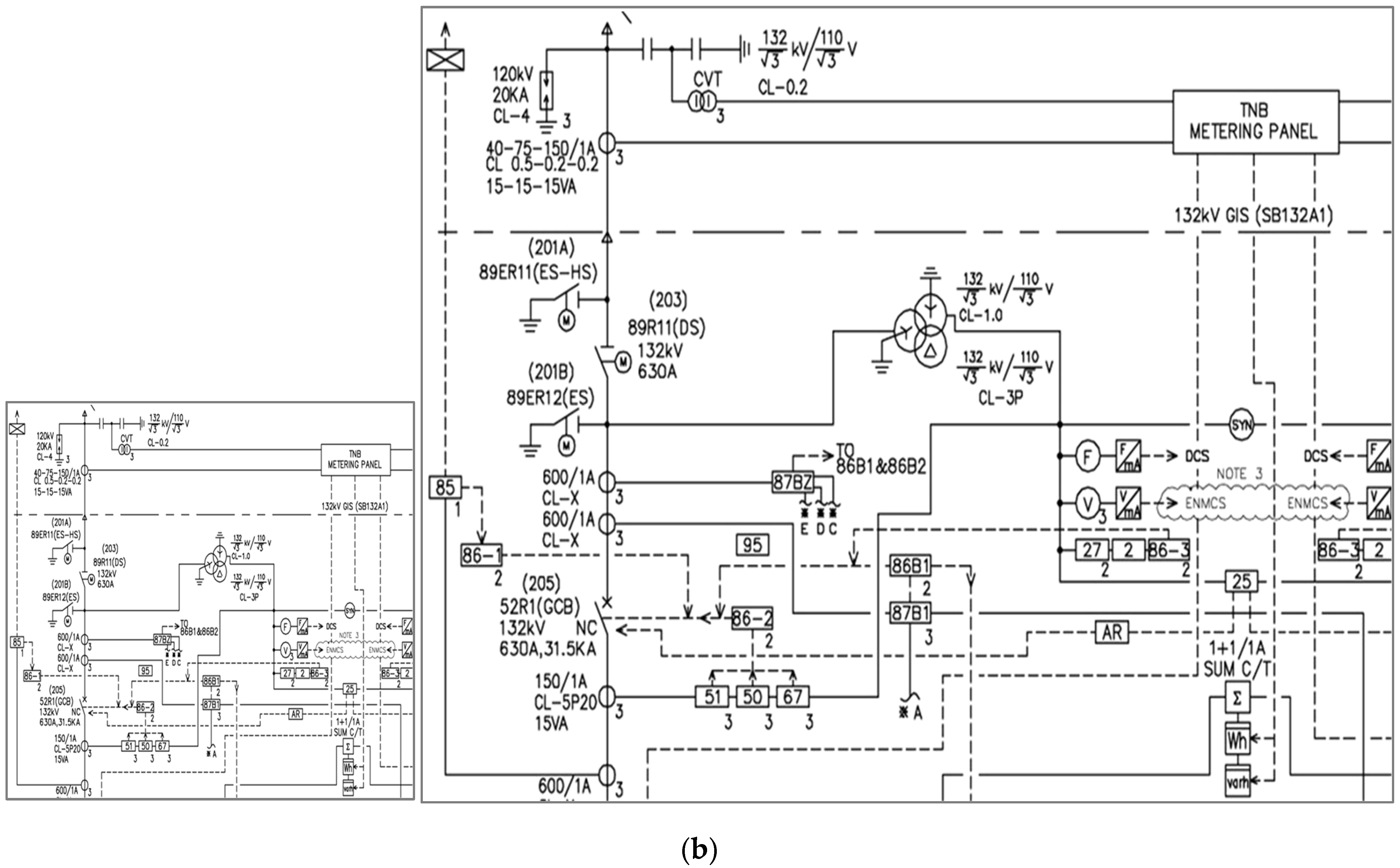
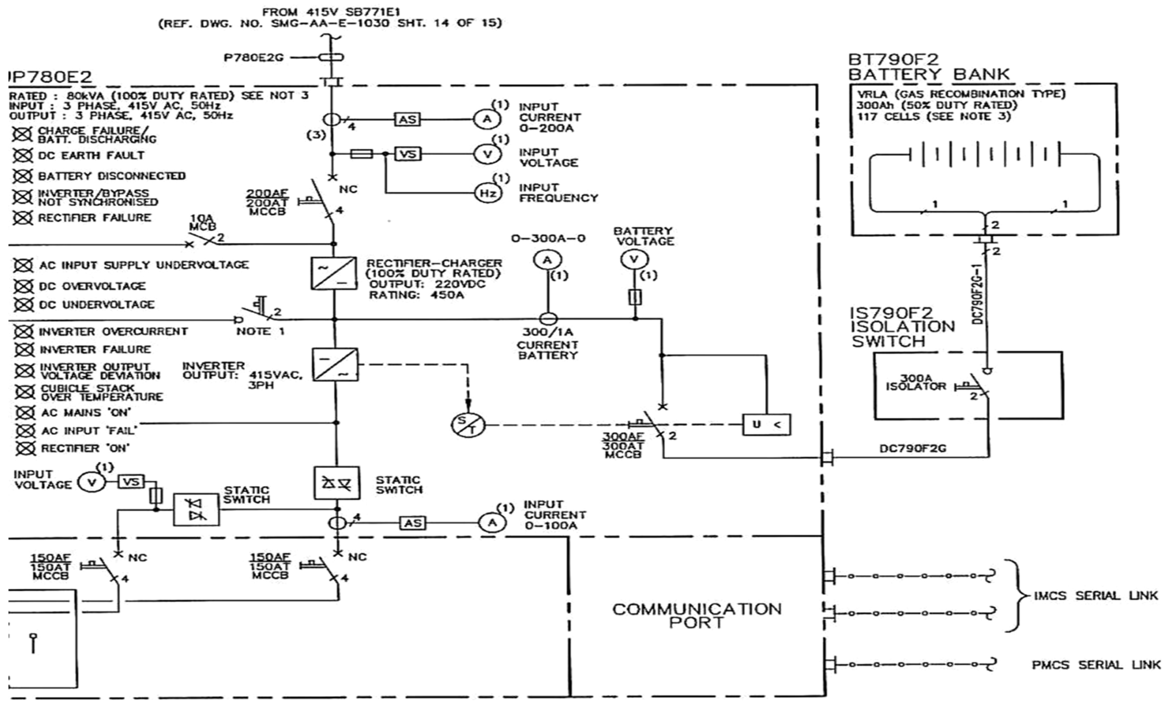
There are numerous industries in which engineering documents continue to exist in paper format due to a lack of digitalization for automated systems [1]. Among such documents, single-line diagrams (SLDs) pose a significant challenge in terms of interpretation and comprehension, as exemplified in Figure 1. These technical documents play a crucial role in diverse fields, including electrical systems, power distribution systems, hazardous area layouts, and other structural layouts. Deciphering these drawings often requires a considerable amount of time and the expertise of highly skilled engineers and professionals [2,3].

Figure 1. A single-line diagram.

The digitization of engineering drawings has gained significant importance in recent years. This is partially due to the pressing need to enhance business procedures, such as equipment monitoring, risk analysis, safety checks, and other operations. It is also driven by the remarkable advancements in computer vision and image understanding, particularly in the fields of gaming and AI [4], NLP [5], health [6], and others. Machine learning and deep learning (DL) [7] have significantly improved performance in various domains. Machine vision, in particular, has greatly benefited from DL [8,9].

Convolutional neural networks (CNNs) have made remarkable progress in recent years and are widely used in various image-related tasks, including biometric-based authentication [10], image classification, handwriting recognition, and object recognition [11]. The advancements in image segmentation, classification, and object recognition prior to CNNs were incremental and limited. However, the introduction of CNNs has completely transformed this field [11]. For example, Taigman et al. introduced the DeepFace facial recognition system, which was first implemented on Facebook in 2014, achieving an accuracy of 97.35%, surpassing conventional systems by approximately 27% [12].

Despite notable advancements in image processing and analysis, the digitization of single-line diagrams (SLDs) and the automated interpretation of these drawings continue to pose significant challenges [13]. Presently, most methods rely on traditional image processing techniques that necessitate manual feature extraction. These approaches are highly domain-specific, susceptible to noise and data distribution variations, and tend to focus on addressing specific aspects of the problem, such as symbol detection or text separation. The performance of these models is greatly influenced by the quality of the provided training data.

Even in challenging and less-controlled environments, fundamental image segmentation and other processing tasks, such as object detection and tracking, have become considerably less difficult. Recent methods, such as faster regions with convolutional neural networks (Faster R-CNNs) [13], single-stage detection (SSD) [14], region-based fully convolutional networks [15], and You Only Look Once (YOLO) [16], have demonstrated high performance in object recognition and classification applications. These methods, along with their extensions, have addressed major obstacles, such as noise, orientation, and image quality, leading to significant advancements in this field of study [17].

Insufficient datasets for the training process pose another significant challenge in the digitization of engineering documents [18]. Deep-learning models require vast numbers of data for effective training. Given the industry’s heavy reliance on manual interpretation of these documents, there has been limited effort in generating the drawings automatically, making it challenging for researchers to acquire labeled data. To tackle this issue, data augmentation techniques have been introduced in recent years [19].

Generative models have also undergone significant advancement and have been effectively used in numerous applications. Generative adversarial networks have recently emerged as some of the most well-known and frequently employed tools for producing content. Ian Goodfellow first presented GANs in 2014 [20]. We will go over our approach based on GANs to solve the issue of an imbalanced dataset in the Methods section. Another difficult issue that affects a wide range of fields, including engineering diagrams, is when several classes of symbols in the drawings are either over-represented or underserved in the dataset [21].

This article provides a comprehensive analysis of the YOLO V5 model for object identification, with a specific focus on one-line symbols. We utilized custom datasets of single-line engineering drawings to locate and classify these symbols. Our dataset consists of 16 distinct categories encompassing typical engineering symbols commonly found in single-line diagrams. To the best of our knowledge, no prior studies have evaluated a substantial number of deep-learning-based object detectors specifically designed for the recognition of single-line symbols, while considering crucial factors, such as precision, recall, and F1 scores.

1.1. Contributions of This Study

This study makes the following key contributions:

• The utilization of a DCGAN and an LSGAN to generate mixed-quality single-line symbols;
• The combination of original and synthetic datasets to create an augmented dataset, thereby improving classification accuracy;
• The proposal of a YOLO-based solution to enhance performance in single-line symbol classification and recognition tasks. As part of this effort, the YOLO V5 training set is expanded by incorporating newly generated synthetic data;
• A comprehensive comparison and analysis of classification accuracy between the original dataset and the augmented dataset.

1.2. Structure of the Study

The structure of this study project is as follows. A discussion of recently published research is presented in Section 2. Section 3 describes the approach that we propose. Section 4 describes the experiments and their results. Section 5 offers a detailed discussion of our findings, and our conclusions and suggestions for additional research are given in Section 6.

2. Related Works

This section covers recent accomplishments made by the research community in this domain. We discuss different deep-learning techniques used for digitizing engineering drawings, and later we present GANs and discuss the general architecture and recent advancements made to improve the performance of GANs.

2.1. Digitization of Engineering Documents

Engineering drawings commonly incorporate diverse forms, symbolic shapes, solid or dashed lines, and text to depict intricate engineering processes in a condensed and comprehensive manner. These technical drawings find extensive application across multiple disciplines. Over the past decade, considerable research efforts have been dedicated to machine vision with the aim of digitizing these sketches [22,23,24,25]. With remarkable progress in computer vision and machine learning, coupled with the existence of vast numbers of undigitized legacy data, the need for a fully automated framework to digitize these drawings has become more imperative than ever before.

One primary limitation of learning methods is their heavy reliance on extensive feature extraction, which is highly dependent on the quality of the extracted features and often lacks generalizability to unobserved instances [26]. The existing literature in this domain has primarily focused on addressing specific aspects of digitizing engineering diagrams, rather than providing a comprehensive and fully automated framework, as indicated by a recent comprehensive review [27]. Some studies have concentrated on the identification and categorization of common symbols in engineering drawings, as well as the separation of text from other graphical elements in diagrams, employing image processing techniques for line identification and deep-learning methods for symbol detection [28]. Alternatively, heuristic strategies have been employed in other studies to locate and classify components in drawings using approaches such as random forests, achieving precision levels exceeding 90% [29], or to discern and differentiate text from graphic elements [30,31,32,33]. However, these approaches may require the modification of heuristic rules or the development of new ones when there are changes to the schematic or symbol representations [34]. Additionally, the effectiveness of these approaches heavily relies on a balanced distribution of data across the dataset.

In recent years, attempts have been made to apply deep-learning-based techniques to tasks similar to the digitization of engineering drawings [35]. Some studies have utilized techniques based on single-stage detection (SSD) to identify doors, windows, and furniture objects in floor-plan diagrams, yielding positive results [36]. However, these studies used small datasets with an insufficient number of furniture items in each drawing [37]. The unbalanced distribution of object classes within these datasets leads to a decline in performance [38,39].

Symbol recognition in process and instrumentation diagrams (P&IDs) is a closely related field. The complexity of P&IDs introduces various challenges in symbol recognition, including adjacent lines, overlapping symbols, unclear regions, and similarity between symbols [40]. A study evaluated four classification tools, namely, multi-stage deep neural networks, hidden Markov models, K-nearest neighbors, and support vector machines (SVMs), using both synthetic and original drawing sheet datasets [41]. Although the SVM model demonstrated the best performance, all techniques involved grouping symbols before classification and removing lines for clearer observation. Additionally, a faster R-CNN was employed to detect and classify handwritten symbols in technical diagrams, with a focus on specific document types, such as PFDs and flowcharts, achieving favorable results compared to traditional methods.

Various frameworks have been proposed for interpreting engineering sheets and P&ID drawings using deep-learning models. The combination of heuristic-based methods with deep-learning techniques has shown promising results in component detection for engineering drawings. A two-stage process was employed, involving Euclidean metrics to connect pipeline tags and symbols, as well as the probabilistic Hough transform for pipeline detection, to localize symbols and text. Another approach utilized a fully linked convolutional neural network to develop symbol localization techniques [42]. A dataset comprising 672 process flow drawings was used to automate engineering drawings, resulting in improved performance compared to conventional methods. However, accurate detection of all components was not achieved, and the class accuracy for different components in the drawings was around 64.0%.

To capture the time-varying signal produced by pen movements during the sketching process of a one-line hand-drawn electrical circuit diagram, hidden Markov models (HMMs) were utilized [43]. A dataset containing 100 hand-drawn sketches was examined for this purpose. The proposed approach, which employed HMMs, yielded promising outcomes. It achieved an accuracy of more than 83% in classifying the points associated with connector and symbol categories correctly.

A circuit-diagram recognition system was developed to address sketch recognition as a dynamic programming problem, incorporating a novel technique called 2D-DP [44]. The 2D-DP technique demonstrated successful identification of interspersed symbols within the sketches. The method introduced a tolerant connectivity function cost, which proved effective in recognizing free-form sketches. The experiment involved analyzing 130 sketches containing ten different types of electrical symbols. Point-level measurements revealed that the novel approach achieved an accuracy of over 90 percent. A grammar-based parsing strategy for recognition of hand-drawn one-line diagrams was introduced to evaluate the system on UML use-case diagrams, showing an improved recognition accuracy [45]. However, further accurate and formal user studies are necessary to understand the strategy’s limitations and explore potential enhancements.

The adoption of advanced deep-learning methodologies has resulted in significant improvements in the detection and recognition of notations and symbols in musical documents [46]. Techniques such as Faster R-CNNs, R-FCNs, YOLO, and SSD have been successfully applied to identify handwritten musical symbols, demonstrating superior performance compared to traditional structured image processing methods for symbol recognition and detection [21,47].

In summary, the existing research highlights a notable gap between the current state of machine learning and technical image comprehension. This discrepancy arises from the rapid progress in the field juxtaposed with the uneven and incremental advancements in a critical application area that has implications across various sectors.

2.2. GAN Networks

Generative adversarial networks (GANs) were first presented by Ian Goodfellow in 2014 [48]. GAN networks are thought of as generative models that can create unique and fresh content [21]. The generator (G) and the discriminator (D) are two competing models (such as CNNs, neural networks, etc.) that make up GANs. The discriminator serves as a classifier that receives input from the generator and the training set (fake input and authentic input). The discriminator will learn how to differentiate between real input samples and fake input samples fed into the network during the training procedure. However, the generator is taught to create samples that accurately reflect the fundamental properties of the original content [49].

As depicted in Figure 2, the generator is a network that uses current data to produce new, realistic pictures. An image is created using random noise z. The generator’s objective is to deceive the discriminator into believing that the fake image it produces is genuine [48]. Equation (1) is a possible way to describe this scenario. When a sample produced by the generator is discriminated against, the generator attempts to reduce the discriminator’s accuracy as much as possible [50].

min_GV(G) = E_z~px(z)[log(1 − D(G(z))]

(1)

Figure 2. The generator.

As seen in Figure 3, the discriminator is a network for differentiating the images. It determines whether an input image is a fake image created by the generator or a genuine image that already exists. The discriminator’s job is to highlight differences between the actual image that already exists and the fake image produced by the generator. Equation (2) is a possible way to describe this. Minimizing the difference between the real data distribution px and the artificial data distribution px(z) is the main goal of GAN training. When discriminating a real sample, the discriminator seeks to optimize accuracy (D(x)), and when separating fake samples from real samples it seeks to maximize 1 − D(G) [50].

max_DV(D) = E_z~px(z)[logD(x)] + E_z~px(z)[log(1 − D(G(z))]

(2)

Figure 3. The discriminator.

The GAN network architecture is depicted in Figure 4, which includes the generator and discriminator. The generator in a GAN is responsible for producing fictitious pictures. To determine which picture is real and which is fake, the discriminator uses either a fake image created by the generator or an already existing real image. The generator and discriminator will evolve in an adversarial manner after thousands of iterations. As a consequence, the generator will be able to produce pictures that resemble actual pictures. This can be stated using the goal function of the GAN (Equation (3)). The discriminator seeks to increase the V value, while the generator seeks to reduce the V value [51].

min_Gmax_DV(D,G) = E_z~px(z)[logD(x)] + E_z~px(z)[log(1 − D(G(z))]

(3)

Figure 4. Generative adversarial networks.

To enhance the overall performance of GANs, numerous study projects have been focused on various GAN variants. BigGAN models were developed by Brock et al. [52] to accomplish the task of producing distinctive images with high resolution from various datasets. The ImageNet dataset’s challenging samples as well as high-resolution images can both be processed by the image identification algorithm. An alternative generator design dubbed StyleGAN was proposed by Karras et al. [53]. The style of the generated image can be dynamically changed based on the most recent data in all convolutional layers thanks to a newly introduced architecture for the generator that the authors created. It aids in directing the complete process of synthesizing pictures, which starts with images of low resolution and progresses to high-resolution images, by beginning with that resolution.

Effective texture synthesis tools called Markovian generative adversarial networks (MGANs) were developed by Wang and Wang [32]. Brown noise can be directly decoded into a realistic texture; on the other hand, these networks can also decode images into the artwork, improving the quality of texture. A GAN-based architecture called spatial GAN (SGAN), which is excellent for generating texture, was developed by Bergmann et al. [34]. This method can combine numerous versatile source photographs to produce diverse textures and produce high-quality texture images.

In order to overcome the GAN’s limitations, the research in [53] explored the use of deep convolutional GANs, which are also referred to as DCGANs. DCGANs address the GAN’s limitations by replacing max-pooling layers with convolutional layers that have larger or fractional strides. This approach facilitates the use of a unified architectural framework to achieve multiple objectives. In the DCGAN model, the generator competes with the discriminator, incentivizing the generator to produce visually appealing images. In certain situations, its instability can make it difficult to apply in various domains due to the structure of the fully connected network.

Another GAN variant, the least-squares generative adversarial network (LSGAN), has two advantages over traditional GANs. Firstly, LSGANs can generate clearer images than regular GANs. Secondly, LSGANs have more consistent success during the learning process. Traditional GANs are unstable during learning, making it difficult to use them in practice [54]. Several recent studies have investigated how the objective function affects the uncertainty of GAN learning.

3. Proposed Method

In this paper, we present our approach for symbol recognition in SLD images. The details of our approach are outlined in Section 3.1, while Section 3.2 provides information on the dataset used for testing, including data exploration and preprocessing techniques. To tackle the class imbalance issue in these drawings, we present our proposed solution in Section 3.3. Furthermore, Section 3.4 elaborates on the object detection method employed in our study.

3.1. SLD Symbol Recognition Method

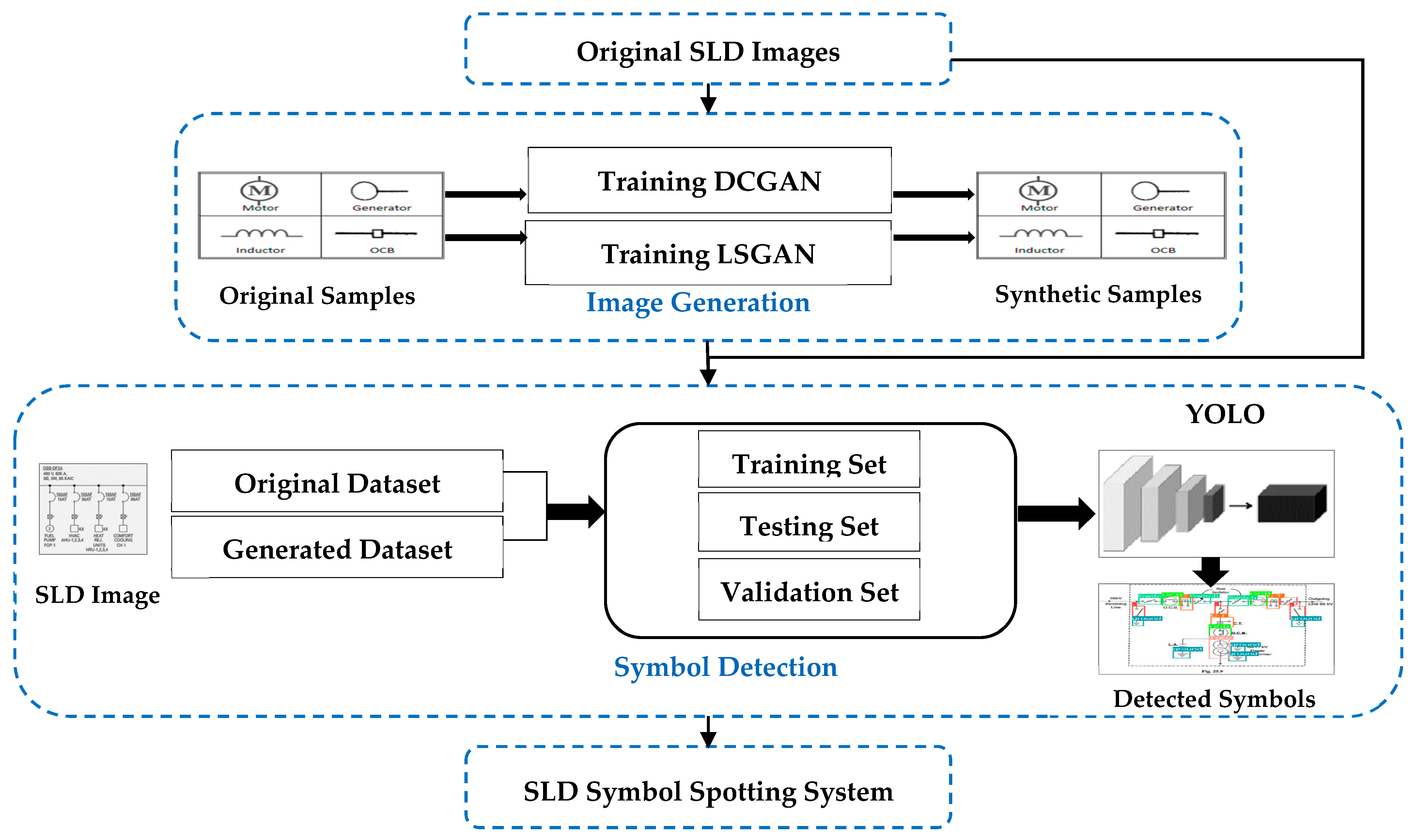
The following section will discuss the process of generating synthetic data for single-line symbol identification in our system using a DCGAN and an LSGAN. A comprehensive illustration of the system’s methodology is presented in Figure 5. The experiment was divided into two parts: (a) the generation of synthetic images through the DCGAN and LSGAN; and (b) the detection of symbols in original and augmented images (combining original images with synthetic images generated by the DCGAN and LSGAN).

Figure 5. The structure of the SLD symbol spotting system.

3.2. Dataset SLD Diagrams

In this article, we chose to conduct experiments using single-line diagrams (SLDs), as shown in Figure 1. For evaluation purposes, our engineering partner provided a collection of 600 sheets containing various types of symbols, lines, and text, as depicted in Figure 6.

Figure 6. Example of individual symbols in a typical SLD.

The SLDs also came in a variety of qualities, which made the dataset appropriate for assessment. The SLD sheets can be viewed as schematic representations of the various electrical system parts and connectivity data. They are illustrations of electrical equipment (often represented as symbols) and power flow movement (represented as various kinds of lines).

These diagrams can be found in many sectors as paper documents or scanned images. It takes a lot of time, effort, and expertise to interpret and analyze these documents [15]. Furthermore, misreading these papers can result in very serious consequences. For instance, if a wire in an electrical system needs to be changed after installation, an engineer must check the corresponding SLD diagram and determine which safety measures must be taken before proceeding with the task. Thus, it is crucial to understand these drawings accurately.

We used GANs to create artificial symbol pictures as part of the data preparation process. The dataset was additionally split into two categories. The first group collection only included actual images. Both the actual images and the generated images created by the DCGAN and LSGAN were included in the second group dataset. The first group dataset only included original pictures, while the other combined the original images with GAN-generated synthetic images, as represented in Table 1.

Table 1. Dataset combinations.

Group	Original Images	Synthetic Images
		DCGAN	LSGAN
1	✓
2	✓	✓	✓

Analysis of SLD Data

The large SLD sheets in the original data measured 7000 by 5000 pixels. We divided the sheet into a 6 × 4 grid to speed up the training, creating 24 patches of sub-images that were relatively small compared to the original pictures (1250 × 1300).

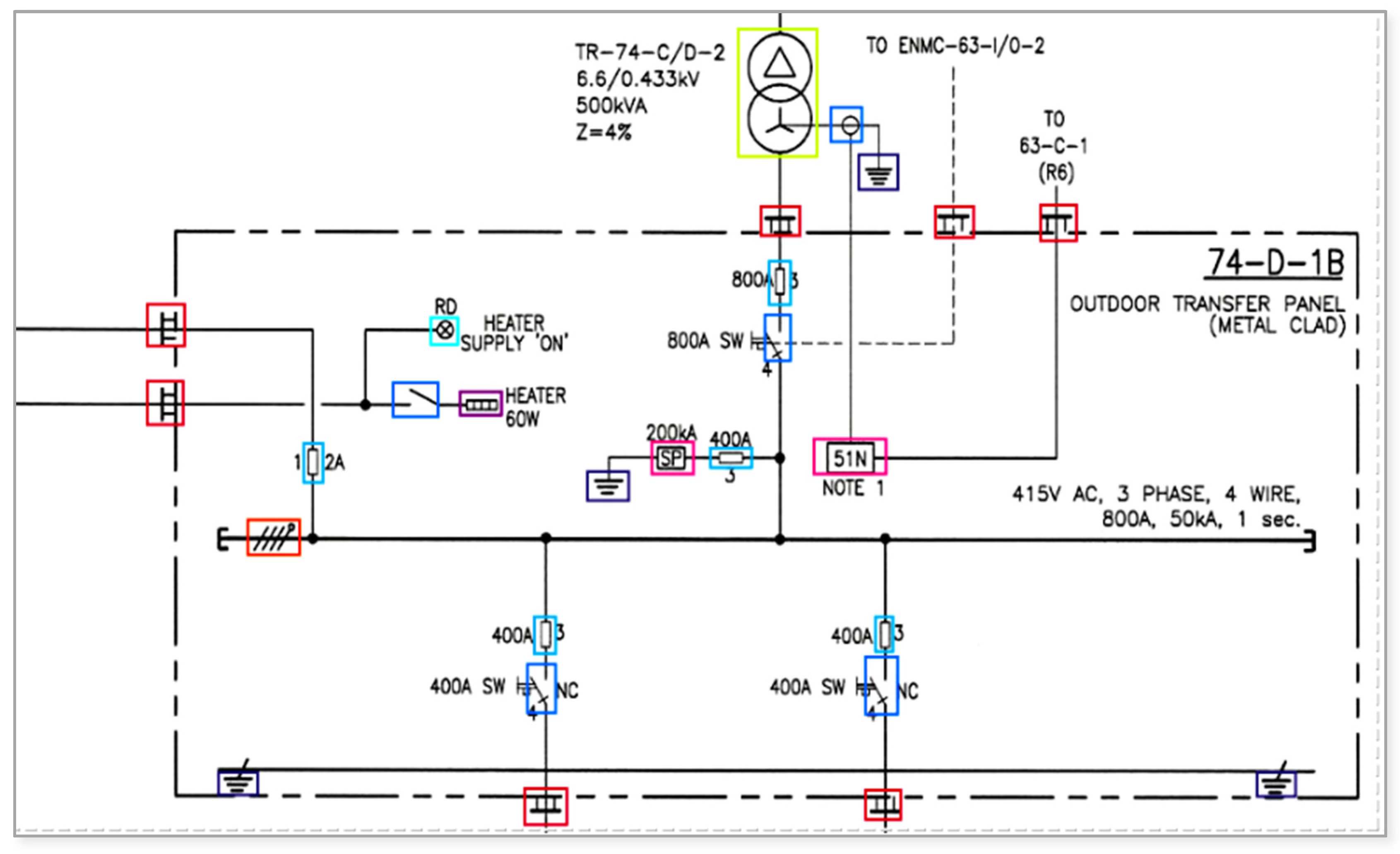
Images and schematics must be completely annotated to prepare a deep-learning model for training. Thus, we annotated the set of SLD images using the RoboFlow tool, which can be seen in Figure 7. In the entire collection, 16 different symbols were annotated. The process of annotating a diagram is straightforward, and in this case involved employing the RoboFlow tool to note the classes of the associated symbols and their locations.

Figure 7. Symbol annotation in part of an SLD image.

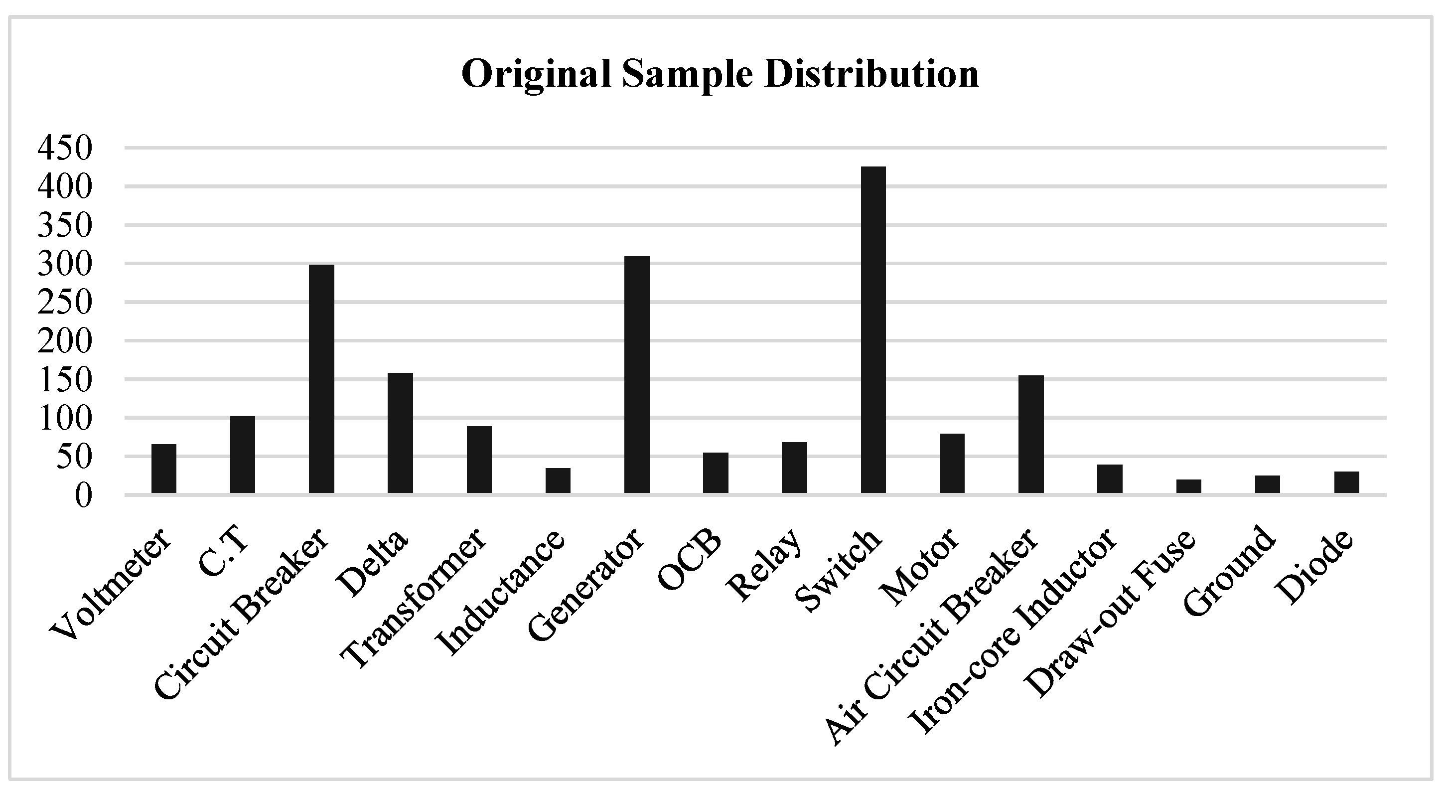
The data that resulted from the annotation were saved in a file that represented the 16 unique classes. The center of the bounding boxes’ x and y values, as well as the widths and heights of the symbols that the bounding boxes enclosed, were captured as data. The collection of 600 images, which included 1953 samples representing 16 various sorts of symbols, was annotated. As can be seen in Figure 8, the original sample was incredibly unbalanced.

Figure 8. Class distribution in the original dataset.

The differences between symbols can be extremely great in some cases. For instance, there are 425 instances of switch symbols in the dataset, compared to just 3 and 6 occurrences of resistor and ammeter symbols, respectively. Fuses and loads only occur 10 times each, although these symbols were excluded from the original dataset due to exceptional under-representation.

3.3. Data Generation by GANs

To ensure that the CNN backbone network of the YOLO V5 model can be trained and classify images by using features from previously illustrated pictures, the DCGAN provides a set of requirements. With its original settings, the DCGAN substitutes the pooling layers on the discriminator and generator with strangled convolutions. CNNs are frequently used to identify traits. Second, to address the gradient disappearance problem, the DCGAN uses the batch normalization method. Every layer in BN has a gradient propagator built in, guaranteeing that the gradient reaches every layer while preventing the generator model from collecting all instances at the respective point. A major concern in this context is that the DCGAN employs various activation functions for various neural networks, including leakyReLU; the ReLU function, which is used for activation; and Adam optimization. The results show that the DCGAN provides better efficiency. When combined with the LSGAN, the DCGAN is generally regarded as the gold standard.

Regarding the images generated by the DCGAN and LSGAN, there were 1000 images of size 32 × 32 and 1000 images of size 64 × 64, respectively, as shown in Table 2, which were then augmented with the original 600 images. The augmented dataset contained a total of 4600 images after merging the original images with the synthetic images.

Table 2. Synthetic image generation using the DCGAN and LSGAN.

Group	Total Images	Generated Image Size (px)	Total Images Generated
1	200	64 × 64	1000
2	200	32 × 32	1000
3	300	64 × 64	1000
4	300	32 × 32	1000

3.3.1. Framework Structure of the DCGAN

In this study, we used the DCGAN to create synthetic pictures of single-line diagrams. The synthetic images were then combined with the LSGAN-generated images and the actual images to increase our dataset and improve the symbol recognition algorithms. Other models improve upon DCGANs by introducing new constraints or by making adjustments.

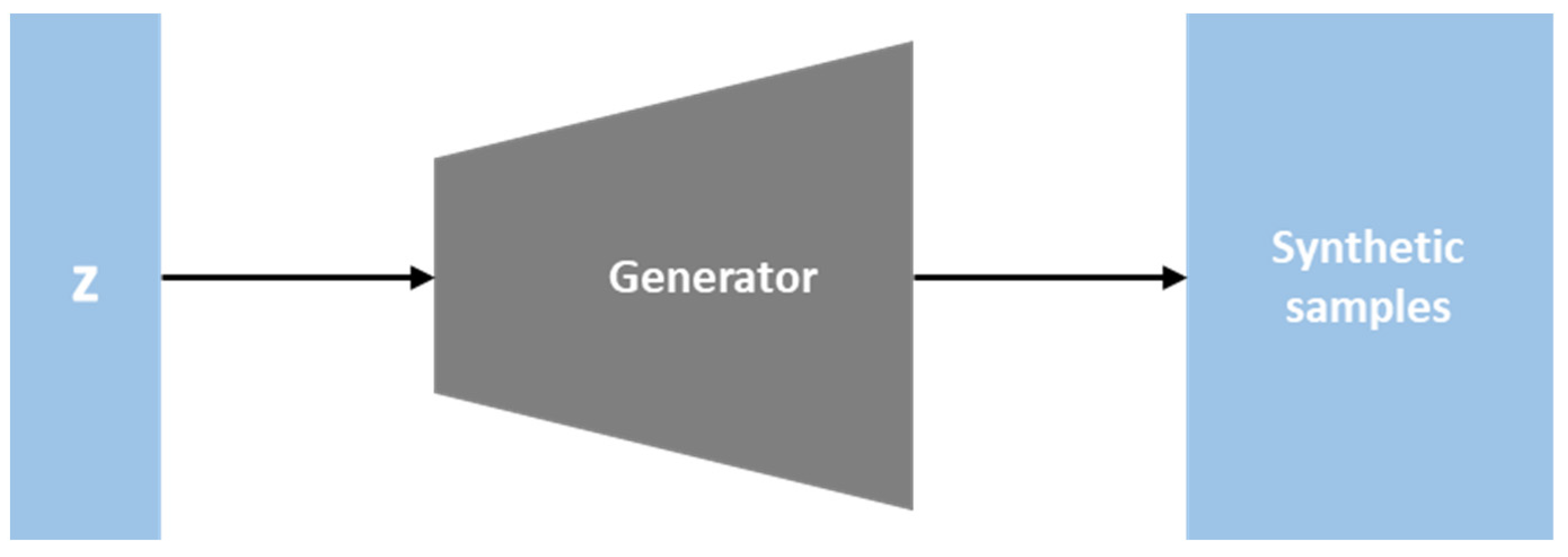
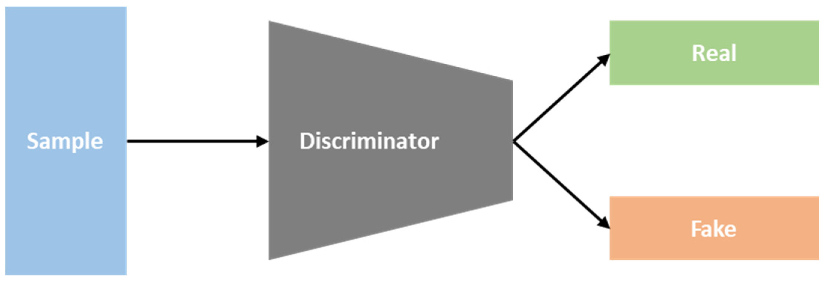
As can be seen in Figure 9, a generative adversarial network consists of a generator module (G) and a discriminator module (D). The generator’s job is to translate a random dataset μ (which it uses as a source) into a desired output dataset φ. The random dataset μ in a conventional GAN is usually uniform or Gaussian noise with a range of zero to one. The discriminator is used to separate the generated outputs φ from the actual datasets φd (the targeted outputs). If the intended outputs are accepted, the discriminator’s D(φd) = 1, while if they are rejected, D(G(μ)) = 0.

Figure 9. Structure of the DCGAN.

Based on a cross-entropy loss function (J(D, G)), the training procedure in a GAN can be viewed as a minimization–maximization problem, as written in Equation (4):

min_Gmax_D = E_{φd~Pdata(φd)}[logD(φ_d)] + E_μ~pμ(μ) [log(1 − D(G(μ)))]

(4)

where p_data(d) is the corresponding probability data distribution for the intended outputs φ_d and pμ(μ) is a prior distribution for the random datasets μ and p_data(φd).

The min–max process involves two steps, as expressed in Equation (5):

J^(D)(θ^(G),θ^(D)) = E_{φd~Pdata(φd)}[logD(φ_d,θ^(D))] + E_μ~pμ(μ)[log(1 − D(G(μ)),θ^(G),θ^(D))]

(5)

where p_data(d) is the corresponding probability data distribution for the intended outputs d and p(d) is a prior distribution for the random dataset.

Changing the generator by minimizing the generator function or min_θ(G)J^(G) θ^(D),θ^(G) (where θ^(G) denotes the parameter in the cost functions of the generator and the function J^(G) is differentiable), yields Equation (6):

J^(D)(θ^(G),θ^(D)) = E_μ~pμ(μ)[log(1 − D(G(μ)))]

(6)

According to Goodfellow et al. [32], if D and G have sufficient capacity, the min–max game has a global optimum for p_g(φ)p_data(φ_d) (where p_g is a probability distribution of the produced output φ when µ~p_µ(µ)). The following characteristics describe the ideal discriminator for the J^(G)(G, D); Equation (7) represents the steps:

$${{\mathrm{D}}^{*}}_{\left(\mathsf{\phi }\mathrm{d}\right)}=\frac{{\mathrm{P}}_{\mathrm{data}\left(\mathsf{\phi }\mathrm{d}\right)}}{{\mathrm{P}}_{\mathrm{data}(\mathsf{\phi }\mathrm{d}+{\mathrm{P}}_{\mathrm{g}}\left(\mathsf{\phi }\right))}}$$

(7)

The calculation of min–max in (3) can be represented in Equation (8) as:

$${\max }_{\mathrm{D}}{\mathrm{J}}^{\left(\mathrm{G}\right)}\left(\mathrm{G},\mathrm{D}\right)={\mathrm{E}}_{\mathsf{\phi }\mathrm{d}~{\mathrm{P}}_{\mathrm{data}\left(\mathsf{\phi }\mathrm{d}\right)}}\left[\log \frac{{\mathrm{P}}_{\mathrm{data}\left(\mathsf{\phi }\mathrm{d}\right)}}{{\mathrm{P}}_{\mathrm{data}(\mathsf{\phi }\mathrm{d}+{\mathrm{P}}_{\mathrm{g}}\left(\mathsf{\phi }\right))}}\right]+{\mathrm{E}}_{\mathsf{\phi }~p_g}[\log \frac{{\mathrm{P}}_{\mathrm{g}\left(\mathsf{\phi }\right)}}{{\mathrm{P}}_{\mathrm{data}(\mathsf{\phi }\mathrm{d}+{\mathrm{P}}_{\mathrm{g}}\left(\mathsf{\phi }\right))}}]$$

(8)

The discriminator loses the ability to differentiate between the actual dataset φ_d and the generated dataset φ when D*_(φd) = $\frac{1}{2}$, which allows the generator to use any random dataset µ to synthesize the generated outputs φ.

The generator’s and discriminator’s parameters θ^(G) and θ^(D) can both be optimized using gradient-based methods.

Due to their poor suitability for storing positional data, DCGANs do not include linear layers or pooling layers. Instead, convolutional networks make up the networks used by DCGANs. The other advantage of a DCGAN is that, when the input data’s layer distribution is biased, it employs batch normalization to correct the mean and variance. The network keeps stacking the convolutional layers until reaching the shape 32 × 32 × 3 with the final transposed convolutional layer, as shown in Figure 9.

3.3.2. Network Structure of the LSGAN

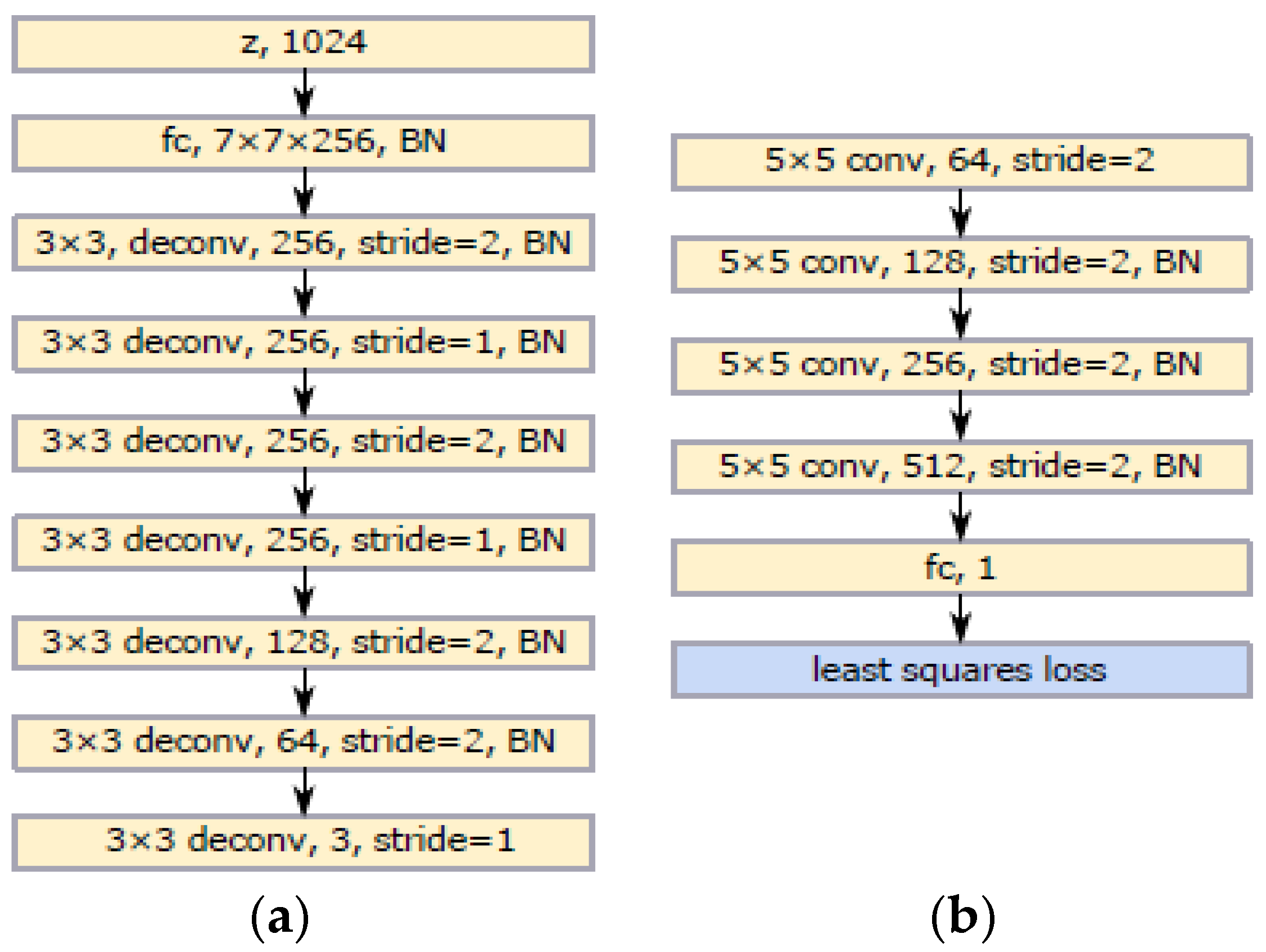
Another GAN variation used for this work is the least-squares GAN (LSGAN), which can be seen in Figure 10. The LSGAN has some benefits over other GANs: (a) the LSGAN improves the initial loss function in the GAN by substituting the least-squares loss function for the original cross-entropy loss function. This technique fixes significant traditional GAN issues; and (b) the LSGAN increases the convergence speed and the training process stability and results in greater image clarity. Similar to conventional GANs, ReLU and Leaky ReLU parameters are used in generators and discriminators. On the other hand, a drawback of the LSGAN is that it results in less sample variety due to excessive penalties for outliers.

Figure 10. Architecture of the LSGAN. (a) The generator of the LSGAN. (b) The discriminator of the LSGAN.

The cost function is readily saturated, so GANs still struggle with the training process’s non-convergence. The “missing modes problems” or “modes collapse” that GANs experience are extremely severe and result in a dearth of variety and generalization. The GAN technique has recently been improved to stabilize training and raise the caliber of the generated samples. For instance, the sigmoid cross-entropy loss used in training caused the gradients in the traditional method to vanish. The least-squares GAN (LSGAN) method [54] replaces the cross-entropy loss by the least-squares function with binary coding to resolve this.

In order to ensure that the generated and real images converge during training, the discriminator’s target values for the real and generated images are represented by labels a and b, respectively. The generator’s target value for the generated images is represented by label c. To achieve this convergence, it is important to select appropriate values for a, b, and c. An extra term is introduced into the generator equation to accomplish this, and since this term is independent of G, the optimal point for the equation remains the same.

The cost function in the LSGAN is given in Equation (9) as:

$${\min }_{\mathrm{D}}{\mathrm{L}}_{\mathrm{LSGAN}}\left(\mathrm{D}\right)=\frac{1}{2}{\mathrm{E}}_{\mathrm{x}~{\mathrm{P}}_{\mathrm{data}}\left(\mathrm{x}\right)}\left[{\left(\mathrm{D}\left(\mathrm{x}\right) - \mathrm{b}\right)}^2\right]+\frac{1}{2}{\mathrm{E}}_{\mathrm{z}~{\mathrm{P}}_{\mathrm{z}}\left(\mathrm{z}\right)}\left[{\left(\mathrm{D}\left(\mathrm{G}\left(\mathrm{z}\right)\right) - \mathrm{a}\right)}^2\right]$$

(9)

The discriminator’s cost function, which is defined by F(D) in Equation (10), can also be transformed into Equation (11).

$${\min }_{\mathrm{D}}{\mathrm{L}}_{\mathrm{LSGAN}}\left(\mathrm{D}\right)=\frac{1}{2}{{\displaystyle \int }}_{\mathrm{x}}{\mathrm{P}}_{\mathrm{data}}\left(\mathrm{x}\right){\left(\mathrm{D}\left(\mathrm{x}\right) - \mathrm{b}\right)}^2 + {\mathrm{P}}_{\mathrm{g}}\left(\mathrm{x}\right){\left(\mathrm{D}\left(\mathrm{x}\right) - \mathrm{a}\right)}^2 \mathrm{dx}$$

(10)

$$\mathrm{F}\left(\mathrm{D}\right)=\frac{1}{2}{\mathrm{P}}_{\mathrm{data}}\left(\mathrm{x}\right){\left(\mathrm{D}\left(\mathrm{x}\right) - \mathrm{b}\right)}^2 + {\mathrm{P}}_{\mathrm{g}}\left(\mathrm{x}\right){\left(\mathrm{D}\left(\mathrm{x}\right)-\mathrm{a}\right)}^2$$

(11)

When the generator is certain and fixed, it is possible to determine the formula for the optimal discriminator as Equation (11) by minimizing the function in Equation (12).

$${{\mathrm{D}}^{*}}_{\left(\mathrm{x}\right)}=\frac{{\mathrm{bP}}_{\mathrm{data}}+\left(\mathrm{x}\right){\mathrm{aP}}_{\mathrm{g}}\left(\mathrm{x}\right)}{{\mathrm{P}}_{\mathrm{data}}\left(\mathrm{x}\right)+{\mathrm{P}}_{\mathrm{g}}\left(\mathrm{x}\right)}$$

(12)

Then, by substituting D*(x), the best generator in terms of optimization can be achieved.

$$\begin{array}{c}2\mathrm{L}\left(\mathrm{G}\right) = {\mathrm{E}}_{\mathrm{x}~{\mathrm{p}}_{\mathrm{data}}} [{{({\mathrm{D}}^{*}}_{\left(\mathrm{x}\right)} - \mathrm{c})}^2] + {\mathrm{E}}_{\mathrm{z}~{\mathrm{p}}_{\mathrm{z}}} \left[{\left({\mathrm{D}}^{*}\left(\mathrm{G}\left(\mathrm{z}\right)\right) - \mathrm{c}\right)}^2\right]={\mathrm{E}}_{\mathrm{x}~{\mathrm{p}}_{\mathrm{data}}} \\ [{\left({{\mathrm{D}}^{*}}_{\left(\mathrm{x}\right)} - \mathrm{c}\right)}^2] + {\mathrm{E}}_{\mathrm{x}~{\mathrm{p}}_{\mathrm{g}}} {\left([{{\mathrm{D}}^{*}}_{\left(\mathrm{x}\right)} - \mathrm{c}\right)}^2]=\\ {{\displaystyle \int }}_{\mathrm{x}}({\mathrm{P}}_{(\mathrm{data}\left(\mathrm{x}\right)+{\mathrm{p}}_{\mathrm{g}}\left(\mathrm{x}\right))}{\left(\frac{\left(\mathrm{b}-\mathrm{c}\right){\mathrm{P}}_{\mathrm{data}}\left(\mathrm{x}\right)\left(\mathrm{a}-\mathrm{c}\right){\mathrm{p}}_{\mathrm{g}}\left(\mathrm{x}\right)}{{\mathrm{P}}_{\mathrm{data}}\left(\mathrm{x}\right) + {\mathrm{P}}_{\mathrm{g}}\left(\mathrm{x}\right)}\right)}^2\mathrm{dx} = \\ {{\displaystyle \int }}_{\mathrm{x}}\frac{\left(\mathrm{b}-\mathrm{c}\right)({\mathrm{P}}_{\mathrm{data}}\left(\mathrm{x}\right){\mathrm{p}}_{\mathrm{g}}\left(\mathrm{x}\right)\left(\mathrm{b}-\mathrm{c}\right){\mathrm{p}}_{\mathrm{g}}\left(\mathrm{x}\right)}{{\mathrm{P}}_{\mathrm{data}}\left(\mathrm{x}\right) + {\mathrm{p}}_{\mathrm{g}}\left(\mathrm{x}\right)})2\mathrm{dx}\end{array}$$

(13)

In reality, there are several sets of viable parameterization options available for LSGANs. A 0–1 binary coding scheme, for instance, can be used to distinguish between generated samples and actual samples when a = 0, b = 1, and c = 1.

In the case where b = 1, a = 1, and c = 0, L (G) is changed to Equation (14):

$$2\mathrm{L}\left(\mathrm{G}\right)={{\displaystyle \int }}_{\mathrm{x}}\frac{{(2\left({\mathrm{p}}_{\mathrm{g}}\left(\mathrm{x}\right)-{\mathrm{P}}_{\mathrm{data}}\left(\mathrm{x}\right){\mathrm{p}}_{\mathrm{g}}\left(\mathrm{x}\right)\right))}^2}{ {\mathrm{P}}_{\mathrm{data}} \left(\mathrm{x}\right) + {\mathrm{p}}_{\mathrm{g}}\left(\mathrm{x}\right)}\mathrm{dx}={\mathrm{X}}_{P_{\mathrm{earson}}}^2({\mathrm{P}}_{\mathrm{data}} + {\mathrm{P}}_{\mathrm{g}}||2{\mathrm{p}}_{\mathrm{g}})$$

(14)

The cost function of the LSGAN in this situation aims to minimize the Pearson difference between p_g+p_data and 2p_g [54]. In this study, the latter criterion is used. Pearson divergence, as well as KL divergence and JS divergence, pertain to the F-divergence family. In statistics, a branch of functions known as F divergence is used to compare two probability density functions—in this instance, the probability density for the generated data (p_g(x)) and the probability density for the real data (P_data(x)). The following is the basic formula for an F-divergence D_f:

$$\mathrm{Df} ({\mathrm{P}}_{\mathrm{g}}\left(\mathrm{x}\right)||{\mathrm{P}}_{\mathrm{data}}\left(\mathrm{x}\right))=\int {\mathrm{p}}_{\mathrm{g}}\left(\mathrm{x}\right)\mathrm{f}\left(\frac{{\mathrm{P}}_{\mathrm{data}}\left(\mathrm{x}\right)}{{\mathrm{p}}_{\mathrm{g}}\left(\mathrm{x}\right)}\right)\mathrm{dx}$$

(15)

F divergence corresponds to KL divergence when f(t) = t logt. F divergence represents ${\mathrm{X}}_{\mathrm{Pearsan}}^2$ divergence when f(t) = (t1)². This change has two advantages that can be seen. Firstly, LSGANs will penalize samples even though they are properly classified, in contrast to GANs which rarely lose data for samples that fall on the right side. The generated samples will travel in the direction of the decision boundary due to the penalization. Secondly, penalizing samples that are far from the decision limit can cause the generator to update with more gradients, solving the issue of vanishing gradients. LSGANs can perform more consistently as a result of the learning process [47].

Information asymmetry, or the fact that there are numerous classes in the input but only one class in the output, is another important factor in mode collapse. Therefore, the labels of the inputs, x_c, are used in G and D to conduct classification when we work with a conditional version of the LSGAN. In our investigation, there were two different types of samples: safe samples and unsafe samples. One-hot encoding was used to binarize the groups. For instance, the secure ones had labels [0, 1], a two-dimensional vector, and the unsafe ones had labels [1, 0]. The one-hot labels xc were added to the end of noisy signals z as the input of G, (z, x_c), represented as the vector of conditional LSGANs.

One-hot labels x_c will be used as the input of D, also known as the vector of (x, x_c), if they are added to the end of reference signals x. The main function becomes:

$$\begin{array}{c}{\min }_{\mathrm{D}}{\mathrm{L}}_{\mathrm{LSGAN}}\left(\mathrm{D}\right)=\frac{1}{2}{\mathrm{E}}_{{\mathrm{x}}_{\mathrm{o}}{\mathrm{x}}_{\mathrm{c}}~{\mathrm{P}}_{\mathrm{data}}\left({\mathrm{x}}_{\mathrm{o}}{\mathrm{x}}_{\mathrm{c}}\right)}\left[{\left(\mathrm{D}\left(\mathrm{x},{\mathrm{x}}_{\mathrm{c}}\right)-1\right)}^2\right]+\frac{1}{2}\\ {\mathrm{E}}_{\mathrm{z}~\mathrm{Pz}\left(\mathrm{z}\right)~{\mathrm{P}}_{\mathrm{data}}}\left({\mathrm{x}}_{\mathrm{o}}{\mathrm{x}}_{\mathrm{c}}\right)\left[{\left(\mathrm{D}\left(\mathrm{G}\left(\mathrm{z},{\mathrm{x}}_{\mathrm{c}}\right),{\mathrm{x}}_{\mathrm{c}}\right)+1\right)}^2\right]\end{array}$$

(16)

$${\min }_{\mathrm{G}}{\mathrm{L}}_{\mathrm{LSGAN}}\left(\mathrm{D}\right)=\frac{1}{2}{\mathrm{E}}_{\mathrm{z}~\mathrm{Pz}\left(\mathrm{z}\right)0\mathrm{xc}~{\mathrm{P}}_{\mathrm{data}}\left(\mathrm{x}0\mathrm{xc}\right)}\left[{\left(\mathrm{D}\left(\mathrm{G}\left(\mathrm{z},{\mathrm{x}}_{\mathrm{c}}\right),{\mathrm{x}}_{\mathrm{c}}\right)\right)}^2\right]$$

(17)

It can be challenging to update the generator when the typical GAN goal functions are reduced because this can lead to gradient-loss issues. The LSGAN gets around this problem by penalizing samples based on how close they are to the decision limit, which causes the generator to update with more gradients. Additionally, theoretical research shows that the training instability of standard GANs is caused by the propensity of the objective function to seek modes, whereas the LSGAN exhibits less mode-seeking activity.

3.4. Symbol Spotting Based on YOLO V5

After merging the images of the single-line diagrams, an object detection technique based on the YOLO model was used in this study to detect and classify the one-line components. The process of YOLO V5, which is frequently used for object detection in surveillance videos, single-line images, face recognition, and other fields, is one of finding and classifying one or more targeted objects in images, as well as determining their classes and positions. The single-line symbol detection task was applied in this study, with satisfying results obtained using the YOLO V5 object recognition algorithm.

The YOLO approach was favored for two key reasons. Firstly, it has a simple architecture that enables the prediction of multiple bounding boxes and class probabilities simultaneously using a single convolutional neural network. Secondly, YOLO is known for its high speed in comparison with other object detection techniques, which is essential for its practical use in testing SLDs that contain an average of 50 engineering symbols.

The Structure of the YOLO V5 Network

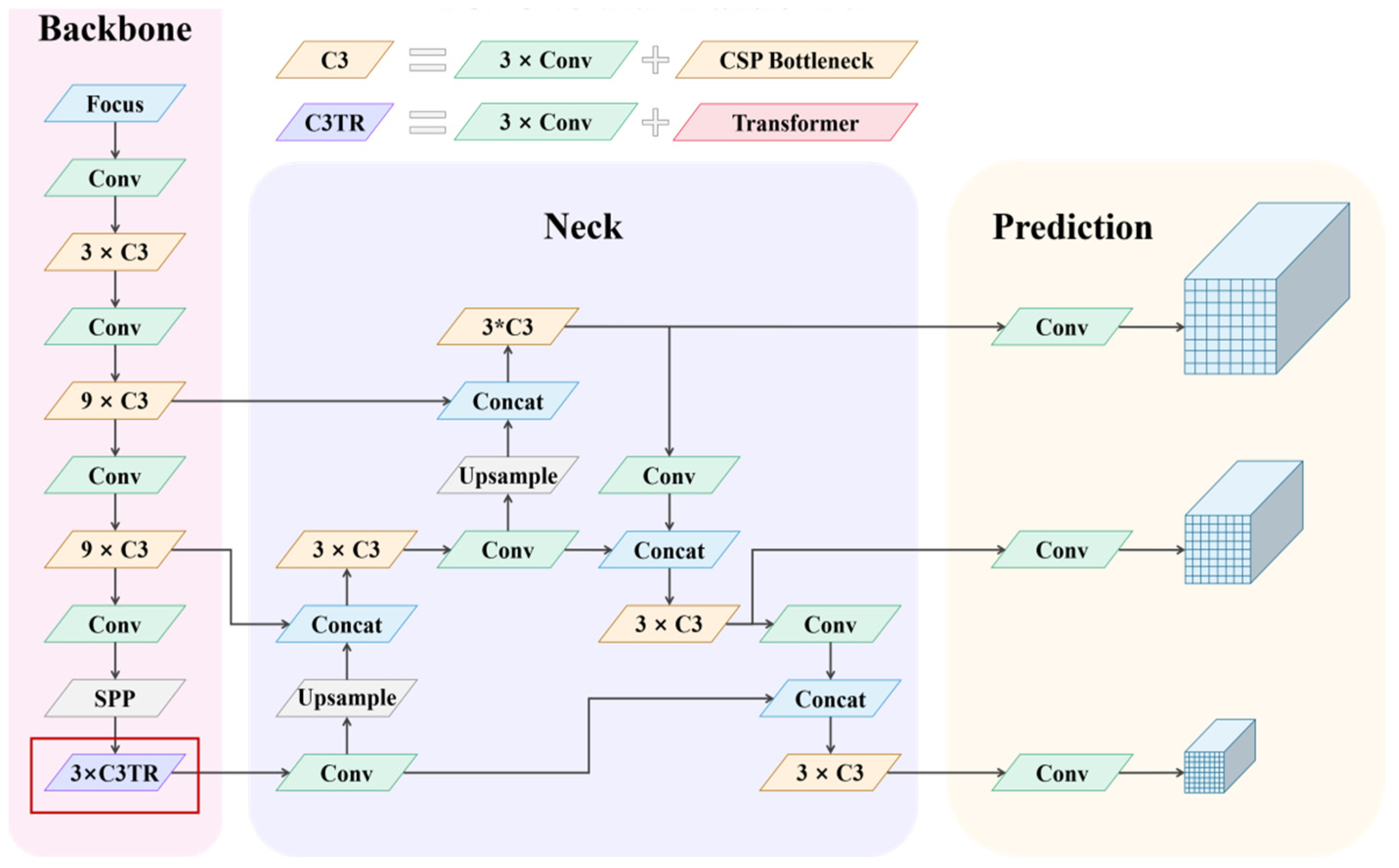
In this study, we used YOLO V5, one of the recent iterations of the YOLO algorithm. YOLO V5 is an efficient and quick object detection algorithm that finds items instantly. Since symbols present in SLDs are very similar to each other, a robust detection speed is also necessary. YOLO V5 is capable of fulfilling this criterion. The deep-learning framework PyTorch, which has outstanding detection performance and has made training and testing for specialized datasets easier, was used to create the algorithm. The backbone, neck, and head are the three components that makeup YOLO V5 [55].

The factors that led us to pick YOLO V5 as the detection model for this study are its simplicity and clarity. To begin with, YOLO V5 merges Darknet with the cross-stage partial network (CSPNet) [43] to produce CSPDarknet, which serves as the network’s core [56,57]. By including gradient changes in the feature map, reducing model parameters and FLOPS (floating-point operations per second), and ensuring inference speed and accuracy while also reducing model size, the CSPNet addresses the issue of recurrent gradient information in large-scale backbones. Speed and accuracy are crucial when detecting sperm cells, and the size of the model affects how well these factors can be inferred using edge devices with restricted resources. Second, to enhance information flow, YOLO V5 uses a path aggregation network (PANet) [15] as its neck. To enhance low-level feature propagation, the PANet employs a novel feature pyramid network (FPN) topology with an improved bottom-up methodology. In addition, adaptive feature sharing, which links the feature grid to all feature levels, makes sure that the subsequent sub-network receives useful information from each feature level. Additionally, the PANet enhances accurate localization signals at lower layers, which greatly increases the accuracy of the object’s location. To provide multi-scale prediction, the YOLO layer, the head of YOLO V5, produces three different sizes of feature maps. The YOLO model can now manage small, medium, and large objects thanks to this.

The CSPNet serves as the framework. Fewer hyper-parameters and FLOPS are produced as a consequence of the CSPNet’s reduction in model complexity. Due to the complexity of the neural networks, it also addresses vanishing and exploding gradient problems. These developments increase the efficiency and precision of object recognition inference. Multiple convolutional layers, three convolutions in four CSP obstacles, and spatial pyramid sharing are all features of the CSPNet. The CSPNet is in charge of extracting features from an input picture and pooling and convolving those features together to create a feature map. As a result, in YOLO V5, the backbone serves as a feature generator.

The neck, or central portion of YOLO V5, is also referred to as the PANet. To execute feature fusions, the PANet collects all the features extracted from the backbone, saves them, and transfers these features to the deep layers. These feature fusions are sent to the head so that the output layer, which will perform the actual object recognition, is aware of the high-level features.

YOLO V5’s head is in charge of object recognition. The target object is surrounded by bounding boxes and a class probability score, which comprises 1 × 1 convolutions that predict the class of an object. The general architecture of YOLO V5 is depicted in Figure 11.

Figure 11. The YOLO V5 network.

Using Equation (18), the bounding box’s position is determined:

$${\mathrm{U}}_{\mathrm{x}}^{\mathrm{y}} = {\mathrm{P}}_{\mathrm{x},\mathrm{y}}\ast {\mathrm{IoU}}_{\mathrm{Predicted}}^{\mathrm{Groun} \mathrm{Truth}}$$

(18)

Equation (18) shows that x and y are the yth bounding rectangle of the xth grid. The probability value for the xth grid’s yth bounding box is U. When there is a subject in the yth bounding box, P_x,y equals 1; otherwise, it equals 0. The intersection over union (IoU) between the expected class and the ground truth is known as the IoU^{ground truth}. More precise predicted bounding boxes are associated with higher IoUs.

The bounding box, categorization, and confidence loss functions are combined to form the YOLO V5 loss function. The total loss function of YOLO V5 is represented by Equation (19) [58]:

loss_YOLOv5 = loss_bounding box + loss_{classification} + loss_confidence

(19)

loss _{bounding box} is calculated using Equation (20):

$${\mathrm{loss}}_{\mathrm{bounding} \mathrm{box}} = {{\mathsf{\lambda }}_{\mathrm{if}} \mathsf{\Sigma }}_{\mathrm{a}=0}^{{\mathrm{b}}^2} {\mathsf{\Sigma }}_{\mathrm{c}=0}^{\mathrm{d}} {\mathrm{E}}_{\mathrm{a},\mathrm{c} }^{\mathrm{g}}, {\mathrm{h}}_{\mathrm{g}}\left(2-{\mathrm{k}}_{\mathrm{a}}{\mathrm{k}}_{\mathrm{na}}\right)\left[{\left({\mathrm{x}}_{\mathrm{a}}-{\mathrm{x}\prime }_{\mathrm{a}}^{\mathrm{c}}\right)}^2+{\left({\mathrm{y}}_{\mathrm{a}}-{\mathrm{y}\prime }_{\mathrm{a}}^{\mathrm{c}}\right)}^2+{\left({\mathrm{w}}_{\mathrm{a}}-{\mathrm{w}\prime }_{\mathrm{a}}^{\mathrm{c}}\right)}^2+{\left({\mathrm{h}}_{\mathrm{a}}-{\mathrm{h}\prime }_{\mathrm{a}}^{\mathrm{c}}\right)}^2\right]$$

(20)

Equation (20) uses h’ and w’ to represent the target object’s breadth and height, while xa and ya stand for the target object’s coordinates in an image. Finally, the indicator function (λif) displays whether the target item is contained within the bounding box.

Equation (21) represents the calculation of loss_{classification}:

$${\mathrm{loss}}_{\mathrm{classification}}={{\mathsf{\lambda }}_{\mathrm{classification}} \mathsf{\Sigma }}_{\mathrm{c}=0}^{{\mathrm{b}}^2}{ \mathsf{\Sigma }}_{\mathrm{c}=0}^{\mathrm{d}}{ \mathrm{E}}_{\mathrm{a},\mathrm{c}}^{\mathrm{g}} {\mathsf{\Sigma }}_{\mathrm{C}Є\mathrm{c}1} {\mathrm{L}}_{\mathrm{a}} \left(\mathrm{c}\right) \log \left({\mathrm{LL}}_{\mathrm{a}}\left(\mathrm{c}\right)\right)$$

(21)

loss _confidence is calculated using Equation (22):

$${\mathrm{loss}}_{\mathrm{confidence}}={{\mathsf{\lambda }}_{\mathrm{confidence}}\mathsf{\Sigma }}_{\mathrm{c}=0}^{{\mathrm{b}}^2}{ \mathsf{\Sigma }}_{\mathrm{c}=0}^{\mathrm{d}}{ \mathrm{E}}_{\mathrm{a},\mathrm{c}}^{\mathrm{Confidence}}{\left({\mathrm{c}}_{\mathrm{i}}-{\mathrm{c}}_{\mathrm{l}}\right)}^2+{ {\mathsf{\lambda }}_{\mathrm{g}} \mathsf{\Sigma }}_{\mathrm{c}=0}^{{\mathrm{b}}^2} {\mathsf{\Sigma }}_{\mathrm{c}=0}^{\mathrm{d}}{ \mathrm{E}}_{\mathrm{a},\mathrm{c}}^{\mathrm{Confidence}}{\left({\mathrm{c}}_{\mathrm{i}}-{\mathrm{c}}_{\mathrm{l}}\right)}^2$$

(22)

The category loss coefficient, λ classification loss λ coefficient, class, and confidence score are all denoted in Equations (21) and (22) by the symbol confidence and classification, respectively.

4. Experiments and Results

In this section, the experimentation environment and procedure are discussed in detail. First, we present the experiments with various GANs and the data generated by the GANs. Second, we present the experiments conducted after having trained YOLO V5 on the original and augmented datasets.

4.1. Data Generation Results

4.1.1. Construction of the SLD Image Dataset

The hyper-parameter was set to 0.5, the batch size was 32, and the layer norm was used as the normalization technique. The training iterations were fixed to 2000. Additionally, the entry and output image sizes were 64 × 64 and 32 × 32, respectively. Using the DCGAN and LSGAN, artificial single-line pictures of sizes (a) 32 × 32 and (b) 64 × 64 were produced and are displayed in Figure 12. Since it is difficult to distinguish between genuine and fake photos, the images were also fairly legitimate. The images appeared to be very clear, authentic, and lifelike. To enhance the performance of the symbol recognition system, the synthetic pictures produced using various GAN methods were to be combined with the real pictures and used for training.

Figure 12. (a) DCGAN-generated images of sizes 32 × 32 and 64 × 64. (b) LSGAN-generated images of sizes 32 × 32 and 64 × 64.

4.1.2. SLD Dataset Distribution

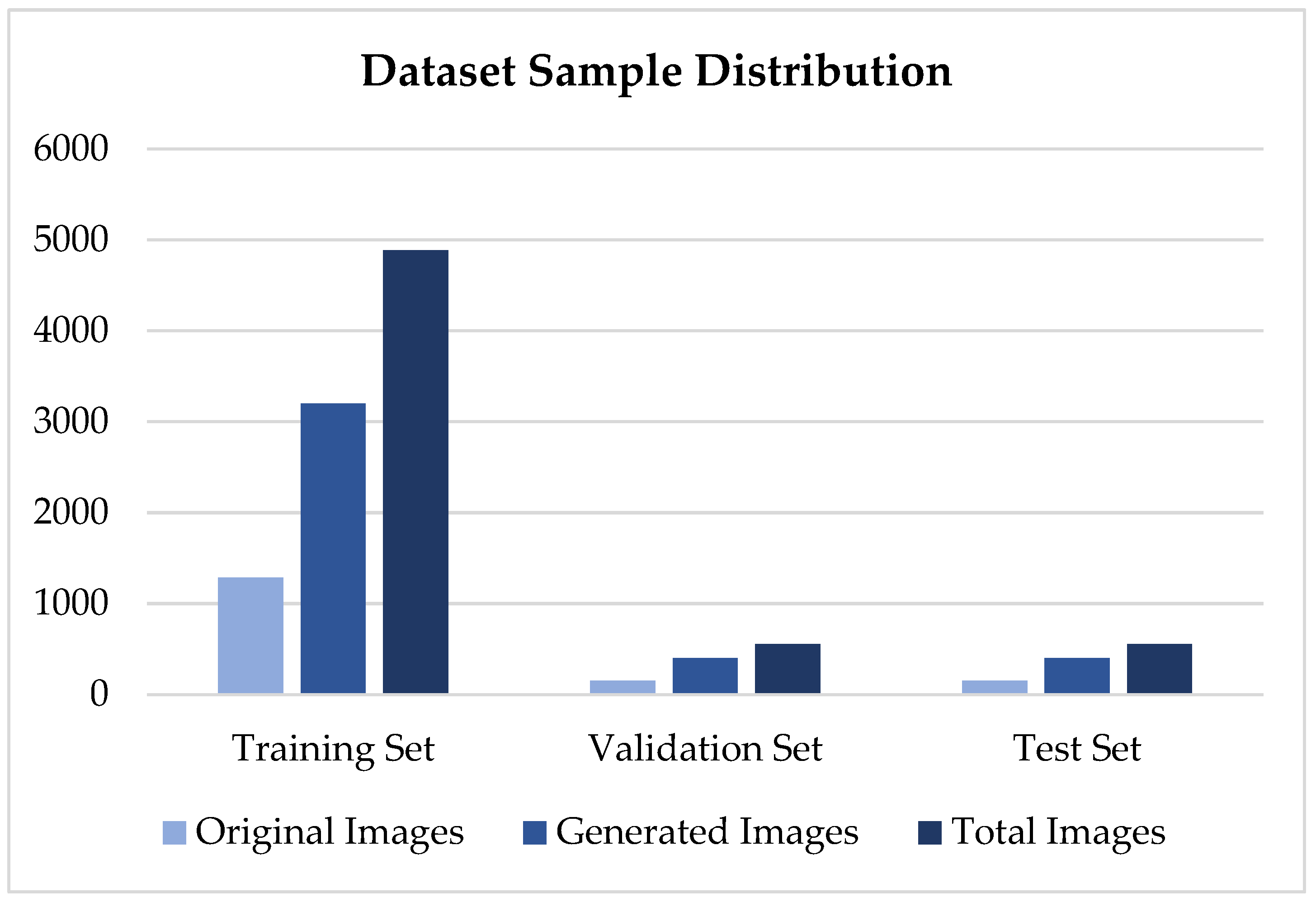
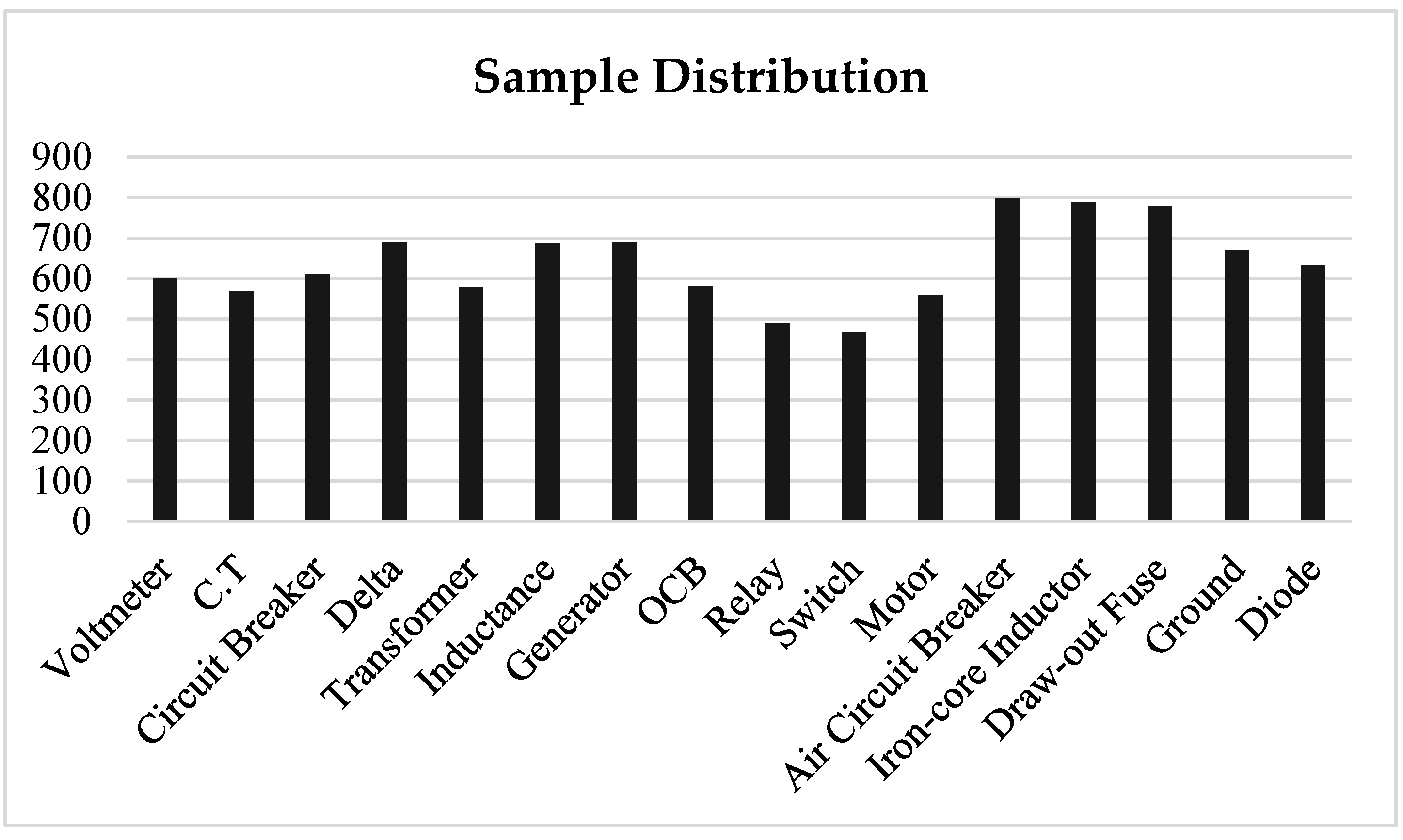
The augmented SLD dataset for the symbol detection model consists of a total of 4600 images with 12,700 samples, which is approximately 6.5 times the size of the original dataset. This dataset includes 690 delta, 560 motor, 689 generator, and 798 air circuit breaker images. The real and synthetic images were divided into three parts in the augmented dataset in a ratio of 6:2:2, which was also used to split the dataset for training, validation, and testing purposes. Figure 13 displays the distribution percentage of the samples.

Figure 13. Proportions of symbol instances in the training, validation, and testing sets.

After data enhancement, a total of 4000 images were generated using the DCGAN and LSGAN. These images consisted of 610 samples of circuit breakers, 468 samples of switches, 600 samples of voltmeters, 687 instances of inductance, and 569 samples of CTs. Each symbol occurred in a well-balanced manner in the new dataset, and the generated samples were plentiful for training the model and achieving satisfactory results. This was demonstrated by the distribution proportion of original to newly produced samples for different symbol types, as shown in Figure 14.

Figure 14. Distribution ratios of original and synthetic samples.

4.2. Evaluation of YOLO V5 Training

4.2.1. Computer Hardware Configuration

Deep-learning networks require robust hardware support. In our case, we utilized a Linux-based system with CUDA 11.1, Python 3.8, and Pytorch 1.8.0. The hardware setup included an Nvidia A40 GPU with 48 GB of memory. This powerful configuration enabled us to efficiently perform all the training and generation operations.

4.2.2. Evolution of Hyper-Parameters

In our study, we enhanced the YOLO V5 model during the training phase by incorporating specific learning rates. We employed learning rates of 0.001 for analysis, 0.1 for each epoch, and 0.9 for the moment. To mitigate overfitting, we employed early stopping and cross-validation techniques. During the experiment, we utilized five-fold cross-validation to obtain out-of-sample forecast errors. The early stopping rules helped us determine the optimal number of iterations before the algorithm became overfitted.

This experiment used the following parameters: max batches = 6000, policy = steps, steps = 6300, 7500, scales = 0.1, 0.1, momentum = 0.958, decay = 0.0004, and mosaic = 1. The largest batches required by m-class object detectors are typically 2000 m. The training procedure in the experiment ended after 8000 rounds (2000 × 4 classes). Additionally, the training procedure made use of the scale (0.1, 0.1) and the present iteration number of 0.001 batches. The learning-rate number was updated regularly and was calculated using a learning-rate scale between [0] and [1] = 0.00001.

The technique used in this paper to optimize the hyper-parameters was based on the genetic algorithm (GA) offered by YOLO V5. The hyper-parameters that were trained on the COCO dataset were the default parameters, and they were programmed to develop once every 50 training epochs for a total of 100 evolutions. As a result, Figure 15’s depiction of the evolution process demonstrates that the ideal collection of hyper-parameters was attained in the 93rd pass. With yellow denoting a higher frequency, the y-axis depicts fitness, the x-axis the values of the hyper-parameters, and the different colors the frequencies of the results. The final hyper-parameter values used for training were initial learning rate lr0 = 0.01199, final learning rate lrf = 0.05053, and SGDmomentum = 0.90091.

Figure 15. Evolution process of the hyper-parameter values.

Since the model alters as the hyper-parameters change, the deep neural network’s hyper-parameters are the external variables that must be manually set and constantly changed to find the ideal combination.

4.2.3. Results and Evaluations

The prediction results of the classification task were classified into four categories based on the relationship between the prediction output and the ground-truth value: (a) True Positive (TP); (b) True Negative (TN); (c) False Positive (FP); and (d) False Negative (FN). This study evaluated the effectiveness of defect detection by calculating the precision, recall, and F1 scores of the detection model for various types of defects. The precision rate reflects the accuracy of the detection findings and is calculated as the ratio of correctly predicted positive samples to all predicted positive samples. The recall rate measures the comprehensiveness of the detection findings and is calculated by dividing the number of correctly predicted positive samples by the total number of actual positive occurrences.

$$\mathrm{Precision} =\frac{\mathrm{TP}}{\mathrm{TP} + \mathrm{FP}}$$

(23)

$$\mathrm{Recall} =\frac{\mathrm{TP}}{\mathrm{TP} + \mathrm{FN}}$$

(24)

The classification issue should consider both the precision of classification and the thoroughness of detection. To assess the model by combining precision and recall, the F1 score is used:

$$\mathrm{F}1-\mathrm{score} =\frac{2}{\frac{1}{\mathrm{Precision}}+\frac{1}{\mathrm{Recall}}}=\frac{2·\mathrm{Precision}·\mathrm{Recall}}{\mathrm{Precision} + \mathrm{Recall}}$$

(25)

Table 3 presents the detection data. Every row represents the predicted category, and every attribute represents the actual class. The overall number of symbols in each category is represented by the sum of each column. The predicted category and the overall number of predicted symbols for each category are shown in each row. Our proposed approach can essentially detect a majority of single-line-based engineering symbols while ensuring accuracy. In this study, the average recall rate was 90.67%, the precision of all kinds of symbol detection was above 90%, and the F1 score was greater than 0.9. The average recollection rate was 90.67%, the average detection time for each frame was 0.074 s, and the average detection time for each frame was 0.074 s.

Table 3. Symbol instances in original and synthetic datasets.

Symbol Name	Original Symbol	Original Instances	Generated Symbol	Generated Instances
Voltmeter		66		600
CT		102		569
Circuit Breaker		298		610
Delta		158		690
Transformer		89		577
Inductance		35		687
Generator		309		689
OCB		55		580
Relay		68		489
Switch		425		468
Motor		79		560
Air Circuit Breaker		155		798
Iron-Core Inductor		39		789
Draw-Out Fuse		20		780
Ground		25		670
Diode		30		633

The model was divided into two groups in this research, each with its own dataset. The second group used both the real images and the DCGAN and LSGAN synthetic images, as opposed to the first group, which only employed actual images. Table 4 displays the training achievement results. Additionally, the Group 2 (original pictures, DCGAN, and LSGAN) dataset achieved the highest mAP of approximately 99.83% with an IoU of 73.11% for YOLO V5. As a consequence, Table 4 shows that combining real and fake images strengthened all models and raised the percentages of IoU and mAP. In this research, the boundary of the real object served as the ground truth to determine how much our predicted border overlapped with it.

Table 4. Training performance results obtained using YOLO V5.

Symbol	Original Dataset				Augmented Dataset
	Samples	Precision	Recall	F1 Score	Samples	Precision	Recall	F1 Score
Voltmeter	66	0.78	0.82	0.77	666	1.00	1.00	1.00
CT	102	0.92	1.00	0.95	671	1.00	0.98	0.98
Circuit Breaker	298	0.78	0.82	0.77	908	1.00	1.00	1.00
Delta	158	0.33	1.00	0.49	848	1.00	1.00	1.00
Transformer	89	0.90	0.77	0.82	666	1.00	1.00	1.00
Inductance	35	0.68	1.00	0.80	722	0.92	1.00	0.95
Generator	309	1.00	0.58	0.73	998	1.00	1.00	1.00
OCB	55	1.00	0.91	0.95	635	1.00	1.00	1.00
Relay	68	0.38	0.01	0.019	557	1.00	1.00	1.00
Switch	425	1.00	0.68	0.80	893	1.00	0.98	0.98
Motor	79	1.00	0.98	0.98	639	1.00	0.98	0.98
Air Circuit Breaker	155	0.56	0.98	0.70	953	1.00	1.00	1.00
Iron-Core Inductor	39	0.56	0.98	0.70	828	1.00	1.00	1.00
Draw-Out Fuse	20	0.33	1.0	0.49	800	1.00	1.00	1.00
Ground	25	0.00	0.00	0.00	695	0.92	1.00	0.95
Diode	30	0.92	1.00	0.95	663	1.00	0.98	0.98

5. Discussion

This section presents a concise and precise description of the experimental results, their interpretation, and the conclusions drawn from the experiments.

5.1. Comparison with Different Data Augmentation Techniques

Table 3 shows the occurrences of 16 different classes present in both datasets. After generating fake SLD images using the DCGAN and LSGAN, it was observed that the new samples were nearly balanced, although the class imbalance problem can be further improved by adding unlike and distinct images to the original dataset.

The detection results of two additional dataset versions, the original SLD images without synthetic images, were compared with the detection results of the augmentation method shown in Table 4. Along with different preprocessing strategies, the subsequent detection networks, including the YOLO V5-based symbol detection model, were consistent.

It is important to acknowledge that enhancing datasets for complex images such as single-line diagrams (SLDs) can present certain challenges. These challenges may include: (i) acquiring authentic SLD images: obtaining SLD images from reliable and trustworthy sources can be problematic; (ii) the manual labor required for labeling the SLD images: labeling SLD images often requires manual effort, as it entails annotating specific elements or regions of interest within the images; and (iii) obtaining a sufficient number of random samples: constructing a comprehensive dataset for SLD images typically requires an adequate number of diverse and random samples. In light of these challenges, the proposed method has demonstrated improvements and offers an alternative approach to address them. By employing the proposed method, it is possible to overcome the difficulties associated with acquiring authentic SLD images by generating a sufficient number of synthetic data, thus reducing the manual labeling effort, and generating a satisfactory number of random samples for a balanced dataset.

5.2. Analysis of the Results

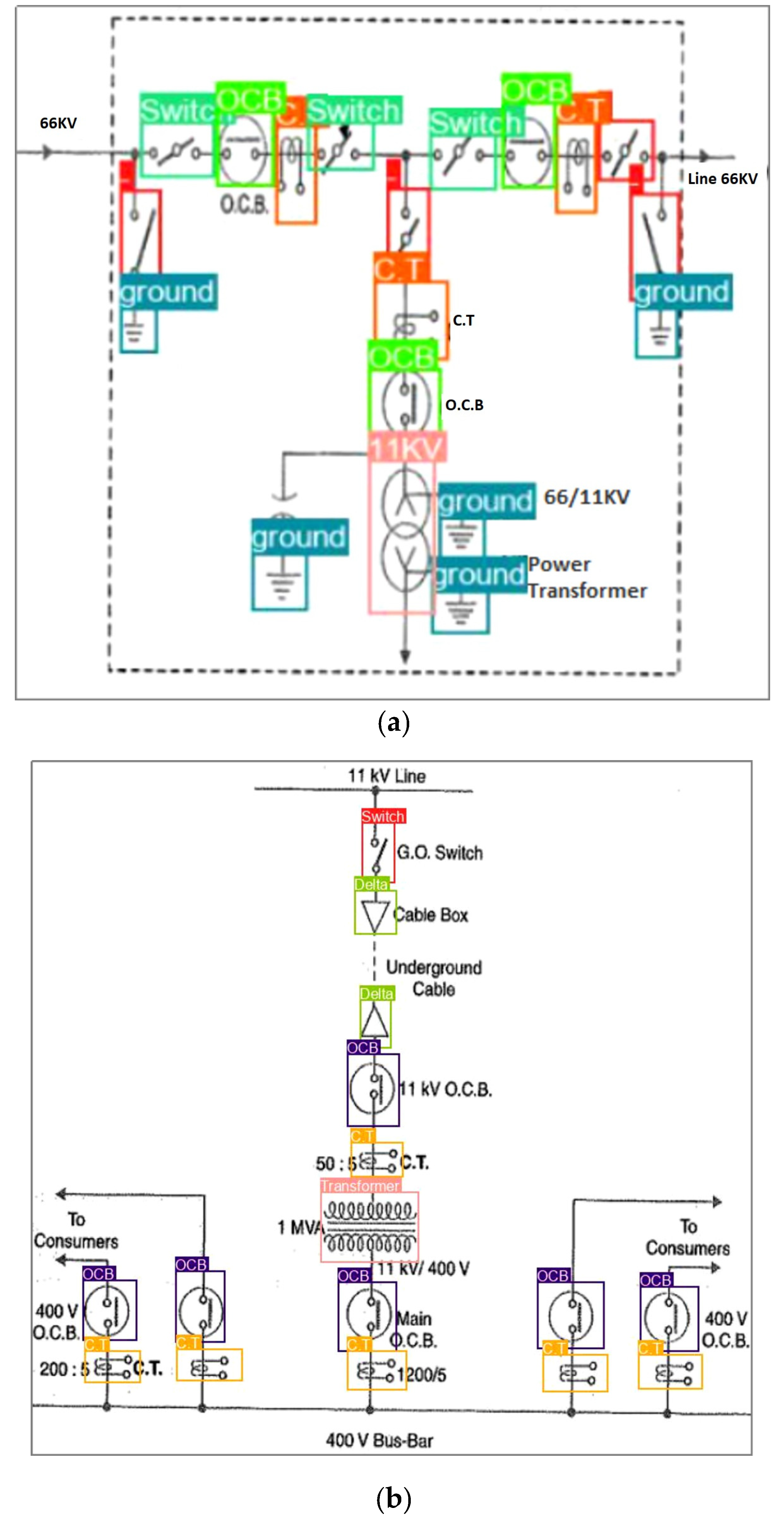
We put YOLO V5 to the test in a variety of settings and configurations using 460 images. A detection example is shown in Figure 16. The testing accuracy findings and experimental performance using images outside of our datasets are shown in Table 5. YOLO V5 is typically more precise than earlier iterations. Group 2 (the augmented dataset) had the greatest average accuracy, with a YOLO V5 model accuracy of 95%. There were only two detection mistakes in Group 2 when using YOLO V5. The performance of YOLO will be enhanced by the large dataset, which includes both the original images and the artificial images produced by GANs. When a deep-learning-based algorithm is trained on a sufficient and adequate dataset, overfitting issues can be reduced to a significant level. Small datasets could be a mapping barrier for neural networks trying to locate an item, although the addition of synthetic samples has several benefits. Firstly, it increases the diversity of the dataset by introducing variations and expanding the range of possible input patterns. This can help the model generalize better and perform well on unseen data. Secondly, synthetic samples can help address issues related to imbalanced classes or rare events by creating additional instances of under-represented data points. This helps to provide more balanced training data and prevent the model from being biased towards the majority class. Finally, synthetic samples can be used to supplement a limited dataset, especially in scenarios where collecting more real data is challenging, time-consuming, or expensive. As a result, adding synthetic images to the dataset along with original images enhances object identification performance.

Figure 16. Detection results for the (a) original dataset and (b) the augmented dataset.

Table 5. YOLO V5 class accuracy for original and augmented datasets.

Dataset	Accuracy	False Detection	Missed Detection
Original	89%	3	4
Augmented	95%	2	0

6. Conclusions

The primary goal of this research was to compare the quality of synthetic images generated by a DCGAN and an LSGAN. The study combined actual SLD images with synthetic images. Various types and quantities of images were used for training purposes. During the experiments, sophisticated bounding-box detection techniques, such as YOLO V5, were utilized and successfully detected symbols from 16 different categories, despite some components having minimal differences. These results indicated the accuracy of the detection technique in challenging tasks.

Our study indicates that incorporating a mix of genuine and synthetic images in the training process enhances the capacity to recognize symbols. We have drawn the following conclusions based on our findings: (1) During the experiment, the dataset that yielded the best results was obtained from Group 2. This dataset involved the combination of authentic images with synthetic images generated through the utilization of DCGAN and LSGAN techniques. (2) Through the integration of real and synthesized images, there was a significant enhancement in recognition performance, resulting in a notable accuracy rate of 95% with YOLO V5. (3) The inclusion of additional samples during the training phase has the potential to enhance performance and minimize errors. To improve object recognition, the dataset should incorporate diverse real and synthetic images.

In the future, our study will concentrate on utilizing GANs to produce symbols in the context of diagrams. This approach is expected to considerably reduce the human effort required for data annotation. Additionally, we will develop a comprehensive system based on the suggested methods to enable the complete processing and analysis of engineering diagrams such as SLDs. We anticipate that the findings presented in this article will make subsequent tasks, such as line detection and text localization, much easier. Moreover, future research will involve combining Explainable AI (XAI) and other GAN techniques, such as WGAN, MCGAN, MFCGAN, and StyleGAN, with additional detection methods.

References

1. Moreno-García, C.F.; Elyan, E.; Jayne, C. Heuristics-Based Detection to Improve Text/Graphics Segmentation in Complex Engineering Drawings. In Proceedings of the Engineering Applications of Neural Networks: 18th International Conference (EANN 2017), Athens, Greece, 25–27 August 2017; pp. 87–98. [Google Scholar] [CrossRef]
2. Bhanbhro, H.; Hassan, S.R.; Nizamani, S.Z.; Bakhsh, S.T.; Alassafi, M.O. Enhanced Textual Password Scheme for Better Security and Memorability. Int. J. Adv. Comput. Sci. Appl. 2018, 9, 1–8. [Google Scholar] [CrossRef][Green Version]
3. Ali-Gombe, A.; Elyan, E. MFC-GAN: Class-imbalanced dataset classification using Multiple Fake Class Generative Adversarial Network. Neurocomputing 2019, 361, 212–221. [Google Scholar] [CrossRef]
4. Elyan, E.; Jamieson, L.; Ali-Gombe, A. Deep learning for symbols detection and classification in engineering drawings. Neural Netw. 2020, 129, 91–102. [Google Scholar] [CrossRef] [PubMed]
5. Huang, R.; Gu, J.; Sun, X.; Hou, Y.; Uddin, S. A Rapid Recognition Method for Electronic Components Based on the Improved YOLO-V3 Network. Electronics 2019, 8, 825. [Google Scholar] [CrossRef]
6. Jamieson, L.; Moreno-Garcia, C.F.; Elyan, E. Deep Learning for Text Detection and Recognition in Complex Engineering Diagrams. In Proceedings of the 2020 International Joint Conference on Neural Networks (IJCNN), Glasgow, UK, 19–24 July 2020; pp. 1–7. [Google Scholar] [CrossRef]
7. Karthi, M.; Muthulakshmi, V.; Priscilla, R.; Praveen, P.; Vanisri, K. Evolution of YOLO-V5 Algorithm for Object Detection: Automated Detection of Library Books and Performace validation of Dataset. In Proceedings of the 2021 International Conference on Innovative Computing, Intelligent Communication and Smart Electrical Systems (ICSES), Chennai, India, 24–25 September 2021; pp. 1–6. [Google Scholar] [CrossRef]
8. Lee, H.; Lee, J.; Kim, H.; Mun, D. Dataset and method for deep learning-based reconstruction of 3D CAD models containing machining features for mechanical parts. J. Comput. Des. Eng. 2021, 9, 114–127. [Google Scholar] [CrossRef]
9. Naosekpam, V.; Sahu, N. Text detection, recognition, and script identification in natural scene images: A Review. Int. J. Multimedia Inf. Retr. 2022, 11, 291–314. [Google Scholar] [CrossRef]
10. Theisen, M.F.; Flores, K.N.; Balhorn, L.S.; Schweidtmann, A.M. Digitization of chemical process flow diagrams using deep convolutional neural networks. Digit. Chem. Eng. 2023, 6, 100072. [Google Scholar] [CrossRef]
11. Wang, J.; Chen, Y.; Dong, Z.; Gao, M. Improved YOLOv5 network for real-time multi-scale traffic sign detection. Neural Comput. Appl. 2022, 35, 7853–7865. [Google Scholar] [CrossRef]
12. Whang, S.E.; Roh, Y.; Song, H.; Lee, J.-G. Data collection and quality challenges in deep learning: A data-centric AI perspective. VLDB J. 2023, 32, 791–813. [Google Scholar] [CrossRef]
13. Guptaa, M.; Weia, C.; Czerniawskia, T. Automated Valve Detection in Piping and Instrumentation (P&ID) Diagrams. In Proceedings of the 39th International Symposium on Automation and Robotics in Construction (ISARC 2022), Bogota, Colombia, 13–15 July 2022; pp. 630–637. [Google Scholar]
14. Bochkovskiy, A.; Wang, C.-Y.; Liao, H.-Y.M. Yolov4: Optimal speed and accuracy of object dtection. arXiv 2020, arXiv:2004.10934. [Google Scholar]
15. Diwan, T.; Anirudh, G.; Tembhurne, J.V. Object detection using YOLO: Challenges, architectural successors, datasets and applications. Multimedia Tools Appl. 2022, 82, 9243–9275. [Google Scholar] [CrossRef] [PubMed]
16. Lee, J.; Hwang, K.-I. YOLO with adaptive frame control for real-time object detection applications. Multimed. Tools Appl. 2022, 81, 36375–36396. [Google Scholar] [CrossRef]
17. Gada, M. Object Detection for P&ID Images using various Deep Learning Techniques. In Proceedings of the 2021 International Conference on Computer Communication and Informatics (ICCCI), Coimbatore, India, 27–29 January 2021; pp. 1–5. [Google Scholar]
18. Zhang, Q.; Zhang, M.; Chen, T.; Sun, Z.; Ma, Y.; Yu, B. Recent advances in convolutional neural network acceleration. Neurocomputing 2018, 323, 37–51. [Google Scholar] [CrossRef]
19. Hong, J.; Li, Y.; Xu, Y.; Yuan, C.; Fan, H.; Liu, G.; Dai, R. Substation One-Line Diagram Automatic Generation and Visualization. In Proceedings of the 2019 IEEE Innovative Smart Grid Technologies-Asia (ISGT Asia), Chengdu, China, 21–24 May 2019; pp. 1086–1091. [Google Scholar] [CrossRef]
20. Ismail, M.H.A.; Tailakov, D. Identification of Objects in Oilfield Infrastructure Using Engineering Diagram and Machine Learning Methods. In Proceedings of the 2021 IEEE Symposium on Computers & Informatics (ISCI), Kuala Lumpur, Malaysia, 16 October 2021; pp. 19–24. [Google Scholar] [CrossRef]
21. Jiang, P.; Ergu, D.; Liu, F.; Cai, Y.; Ma, B. A Review of Yolo algorithm developments. Procedia Comput. Sci. 2022, 199, 1066–1073. [Google Scholar] [CrossRef]
22. Liu, X.; Meng, G.; Pan, C. Scene text detection and recognition with advances in deep learning: A survey. Int. J. Doc. Anal. Recognit. (IJDAR) 2019, 22, 143–162. [Google Scholar] [CrossRef]
23. Mani, S.; Haddad, M.A.; Constantini, D.; Douhard, W.; Li, Q.; Poirier, L. Automatic Digitization of Engineering Diagrams using Deep Learning and Graph Search. In Proceedings of the 2020 IEEE/CVF Conference on Computer Vision and Pattern Recognition Workshops (CVPRW), Seattle, WA, USA, 14–19 June 2020; pp. 673–679. [Google Scholar]
24. Moreno-García, C.F.; Elyan, E.; Jayne, C. New trends on digitisation of complex engineering drawings. Neural Comput. Appl. 2018, 31, 1695–1712. [Google Scholar] [CrossRef]
25. Nguyen, T.; Van Pham, L.; Nguyen, C.; Van Nguyen, V. Object Detection and Text Recognition in Large-scale Technical Drawings. In Proceedings of the 10th International Conference on Pattern Recognition Applications and Methods (Icpram), Vienna, Austria, 17 December 2021; pp. 612–619. [Google Scholar]
26. Nurminen, J.K.; Rainio, K.; Numminen, J.-P.; Syrjänen, T.; Paganus, N.; Honkoila, K. Object detection in design diagrams with machine learning. In Proceedings of the International Conference on Computer Recognition Systems, Polanica Zdroj, Poland, 20–22 May 2019; pp. 27–36. [Google Scholar]
27. Redmon, J.; Divvala, S.; Girshick, R.; Farhadi, A. You only look once: Unified, real-time object detection. In Proceedings of the IEEE Conference on Computer Vision and Pattern Recognition, Las Vegas, NV, USA, 27–30 June 2016; pp. 779–788. [Google Scholar]
28. Rezvanifar, A.; Cote, M.; Albu, A.B. Symbol Spotting on Digital Architectural Floor Plans Using a Deep Learning-based Framework. In Proceedings of the 2020 IEEE/CVF Conference on Computer Vision and Pattern Recognition Workshops (CVPRW), Seattle, WA, USA, 14–19 June 2020; pp. 2419–2428. [Google Scholar] [CrossRef]
29. Sarkar, S.; Pandey, P.; Kar, S. Automatic Detection and Classification of Symbols in Engineering Drawings. arXiv 2022, arXiv:2204.13277. [Google Scholar]
30. Shetty, A.K.; Saha, I.; Sanghvi, R.M.; Save, S.A.; Patel, Y.J. A review: Object detection models. In Proceedings of the 2021 6th International Conference for Convergence in Technology (I2CT), Maharashtra, India, 2–4 April 2021; pp. 1–8. [Google Scholar]
31. Shin, H.-J.; Jeon, E.-M.; Kwon, D.-k.; Kwon, J.-S.; Lee, C.-J. Automatic Recognition of Symbol Objects in P&IDs using Artificial Intelligence. Plant J. 2021, 17, 37–41. [Google Scholar]
32. Wang, Q.S.; Wang, F.S.; Chen, J.G.; Liu, F.R. Faster R-CNN Target-Detection Algorithm Fused with Adaptive Attention Mechanism. Laser Optoelectron P 2022, 12, 59. [Google Scholar] [CrossRef]
33. Wen, L.; Jo, K.-H. Fast LiDAR R-CNN: Residual Relation-Aware Region Proposal Networks for Multiclass 3-D Object Detection. IEEE Sens. J. 2022, 22, 12323–12331. [Google Scholar] [CrossRef]
34. Yu, E.-S.; Cha, J.-M.; Lee, T.; Kim, J.; Mun, D. Features Recognition from Piping and Instrumentation Diagrams in Image Format Using a Deep Learning Network. Energies 2019, 12, 4425. [Google Scholar] [CrossRef]
35. Denton, E.L.; Chintala, S.; Fergus, R. Deep generative image models using a laplacian pyramid of adversarial networks. Adv. Neural Inf. Process. Syst. 2015. [Google Scholar]
36. Dong, Q.; Gong, S.; Zhu, X. Class rectification hard mining for imbalanced deep learning. In Proceedings of the IEEE International Conference on Computer Vision, Venice, Italy, 22–29 October 2017; pp. 1851–1860. [Google Scholar]
37. Dosovitskiy, A.; Springenberg, J.T.; Riedmiller, M.; Brox, T. Discriminative unsupervised feature learning with convolutional neural networks. Adv. Neural Inf. Process. Syst. 2014. [CrossRef] [PubMed]
38. Fernández, A.; López, V.; Galar, M.; del Jesus, M.J.; Herrera, F. Analysing the classification of imbalanced data-sets with multiple classes: Binarization techniques and ad-hoc approaches. Knowledge-Based Syst. 2013, 42, 97–110. [Google Scholar] [CrossRef]
39. Frid-Adar, M.; Klang, E.; Amitai, M.; Goldberger, J.; Greenspan, H. Synthetic data augmentation using GAN for improved liver lesion classification. In Proceedings of the 2018 IEEE 15th International Symposium on Biomedical Imaging (ISBI 2018), Washington, DC, USA, 4–7 April 2018; pp. 289–293. [Google Scholar] [CrossRef]
40. Yun, D.-Y.; Seo, S.-K.; Zahid, U.; Lee, C.-J. Deep Neural Network for Automatic Image Recognition of Engineering Diagrams. Appl. Sci. 2020, 10, 4005. [Google Scholar] [CrossRef]
41. Zhang, Z.; Xia, S.; Cai, Y.; Yang, C.; Zeng, S. A Soft-YoloV4 for High-Performance Head Detection and Counting. Mathematics 2021, 9, 3096. [Google Scholar] [CrossRef]
42. Zhao, Z.-Q.; Zheng, P.; Xu, S.-T.; Wu, X. Object detection with deep learning: A review. IEEE Trans. Neural Netw. Learn. Syst. 2019, 30, 3212–3232. [Google Scholar] [CrossRef]
43. Costagliola, G.; Deufemia, V.; Risi, M. A Multi-layer Parsing Strategy for On-line Recognition of Hand-drawn Diagrams. In Proceedings of the Visual Languages and Human-Centric Computing (VL/HCC’06), Brighton, UK, 4–8 September 2006; pp. 103–110. [Google Scholar] [CrossRef]
44. Feng, G.; Viard-Gaudin, C.; Sun, Z. On-line hand-drawn electric circuit diagram recognition using 2D dynamic programming. Pattern Recognit. 2009, 42, 3215–3223. [Google Scholar] [CrossRef]
45. Zhang, Y.; Viard-Gaudin, C.; Wu, L. An Online Hand-Drawn Electric Circuit Diagram Recognition System Using Hidden Markov Models. In Proceedings of the 2008 International Symposium on Information Science and Engineering, Shanghai, China, 20–22 December 2008; Volume 2, pp. 143–148. [Google Scholar] [CrossRef]
46. Luque, A.; Carrasco, A.; Martín, A.; de Las Heras, A. The impact of class imbalance in classification performance metrics based on the binary confusion matrix. Pattern Recognit. 2019, 91, 216–231. [Google Scholar] [CrossRef]
47. Douzas, G.; Bacao, F. Effective data generation for imbalanced learning using conditional generative adversarial networks. Expert Syst. Appl. 2018, 91, 464–471. [Google Scholar] [CrossRef]
48. Baur, C.; Albarqouni, S.; Navab, N. MelanoGANs: High resolution skin lesion synthesis with GANs. arXiv 2018, arXiv:1804.04338. [Google Scholar]
49. Antoniou, A.; Storkey, A.; Edwards, H. Data Augmentation Generative Adversarial Networks. arXiv 2017, arXiv:1711.04340. [Google Scholar] [CrossRef]
50. He, K.; Zhang, X.; Ren, S.; Sun, J. Deep residual learning for image recognition. In Proceedings of the IEEE Conference on Computer Vision and Pattern Recognition, Conference on Computer Vision and Pattern Recognition (CVPR), Las Vegas, NV, USA, 27–30 June 2016; pp. 770–778. [Google Scholar]
51. Huang, C.; Li, Y.; Loy, C.C.; Tang, X. Learning deep representation for imbalanced classification. In Proceedings of the IEEE Conference on Computer Vision and Pattern Recognition, Las Vegas, NV, USA, 27–30 June 2016; pp. 5375–5384. [Google Scholar]
52. Inoue, H. Data augmentation by pairing samples for images classification. arXiv 2018, arXiv:1801.02929. [Google Scholar]
53. Karras, T.; Aila, T.; Laine, S.; Lehtinen, J. Progressive growing of gans for improved quality, stability, and variation. arXiv 2017, arXiv:1710.10196. [Google Scholar]
54. Mariani, G.; Scheidegger, F.; Istrate, R.; Bekas, C.; Malossi, C. Bagan: Data augmentation with balancing gan. arXiv 2018, arXiv:1803.09655. [Google Scholar]
55. Odena, A. Semi-supervised learning with generative adversarial networks. arXiv 2016, arXiv:1606.01583. [Google Scholar]
56. Wan, L.; Wan, J.; Jin, Y.; Tan, Z.; Li, S.Z. Fine-Grained Multi-Attribute Adversarial Learning for Face Generation of Age, Gender and Ethnicity. In Proceedings of the 2018 International Conference on Biometrics (ICB), Gold Coast, QLD, Australia, 20–23 February 2018; pp. 98–103. [Google Scholar] [CrossRef]
57. Yue, Y.; Liu, H.; Meng, X.; Li, Y.; Du, Y. Generation of High-Precision Ground Penetrating Radar Images Using Improved Least Square Generative Adversarial Networks. Remote Sens. 2021, 13, 4590. [Google Scholar] [CrossRef]
58. Uzun, C.; Çolakoğlu, M.B.; İnceoğlu, A. GAN as a generative architectural plan layout tool: A case study for training DCGAN with Palladian Plans and evaluation of DCGAN outputs. A|Z ITU J. Fac. Arch. 2020, 17, 185–198. [Google Scholar] [CrossRef]
Disclaimer/Publisher’s Note: The statements, opinions and data contained in all publications are solely those of the individual author(s) and contributor(s) and not of MDPI and/or the editor(s). MDPI and/or the editor(s) disclaim responsibility for any injury to people or property resulting from any ideas, methods, instructions or products referred to in the content.
Article Metrics
Citations
Article Access Statistics
Multiple requests from the same IP address are counted as one view.