Article

Maximum Correntropy Square-Root Cubature Kalman Filter with State Estimation for Distributed Drive Electric Vehicles

1
College of Mechanical and Electronic Engineering, Dalian Minzu University, Dalian 116600, China
2
School of Automotive Engineering, Dalian University of Technology, Dalian 116024, China
*
Author to whom correspondence should be addressed.
Appl. Sci. 2023, 13(15), 8762; https://doi.org/10.3390/app13158762
Submission received: 30 June 2023 / Revised: 21 July 2023 / Accepted: 27 July 2023 / Published: 29 July 2023
(This article belongs to the Special Issue Intelligent Vehicles and Autonomous Driving)

Abstract

:
For nonlinear systems, both the cubature Kalman filter (CKF) and square-root cubature Kalman filter (SCKF) can get good estimation performance under Gaussian noise. However, the actual driving environment noise mostly has non-Gaussian properties, leading to a significant reduction in robustness and accuracy for distributed vehicle state estimation. To address such problems, this paper uses the square-root cubature Kalman filter with the maximum correlation entropy criterion (MCSRCKF), establishing a seven degrees of freedom (7-DOF) nonlinear distributed vehicle dynamics model for accurately estimating longitudinal vehicle speed, lateral vehicle speed, yaw rate, and wheel rotation angular velocity using low-cost sensor signals. The co-simulation verification is verified by the CarSim/Simulink platform under double-lane change and serpentine conditions. Experimental results show that the MCSRCKF has high accuracy and enhanced robustness for distributed drive vehicle state estimation problems in real non-Gaussian noise environments.

1. Introduction

Automotive energy saving, environmental protection, and safety technologies are the core aspects of the world’s automotive technology innovation, and automotive active safety control systems are essential for the future survival and development of automotive enterprises [1]. As one of the new energy vehicles, distributed-drive electric vehicles have become an important direction for electric vehicle development because of their unique advantages and huge development potential in power configuration, transmission structure, handling performance, and energy utilization. Obtaining key operating parameters for distributed-drive electric vehicles is essential to achieving system control, such as the longitudinal velocity, lateral velocity, and yaw rate of the vehicle, etc. However, such key information cannot be directly measured by sensors and other equipment. On the one hand, sensors measuring these parameters are influenced by environmental factors and are too demanding for installation conditions; on the other hand, the presence of non-Gaussian noise in real environments deteriorates the general estimation algorithms. Therefore, it is necessary to use on-board sensors in combination with appropriate algorithms for the estimation and identification of vehicle status [2,3].
The Kalman filter (KF) algorithm is mostly used in practical estimation. Marco, V.R. et al. established a KF and recursive least squares method for adaptive observers to accurately estimate the vehicle driving state, but the algorithm design is complicated and has limitations because KF cannot adapt to nonlinear models and the amount of calculation of the least squares algorithm increases gradually with iterative operation [4]. Hu et al. introduced limited memory filtering and random weighting theory in the extended Kalman filter (EKF) for algorithm adaptability. Using the limited memory filter allows adjusting the weights for old and new data, thus reducing the estimation error caused by inaccurate models, and random weighting theory improves the accuracy of the algorithm by introducing random weighting factors to increase the utilization of new measurements in the filtering system. However, the linearization process of EKF performs Taylor expansion and then rounds off the second-order and higher terms, thus generating truncation errors as well as requiring the computation of a cumbersome Jacobian matrix, which can lead to accuracy degradation and filter scattering under high-dimensional systems [5].
Julier and Uhlmann et al. presented the unscented Kalman filter (UKF) for this issue, which selects sigma sample points based on the Gaussian distribution property, does not need to compute complex Jacobi matrices, does not require linearization of the state equation, does not have truncation error, and offers more accurate and efficient performance [6]. Wan et al. combined Huber’s method with the UKF. By introducing the Huber cost function for real-time correction of measurement noise, the effect of irregular errors and noise is effectively suppressed while obtaining higher observation accuracy [7]. When selecting the sigma sample points of UKF, the average value at the center carries more weight, and its accuracy is very important, while UKF may diverge or decrease in accuracy in high-dimensional state spaces [8].
To solve this issue, Arasaratnam and Haykin came up with the CKF, which is cubature transformation-based. The CKF is insensitive to dimensional increase and uses the ball cube rule to select the cubature points [9], which overcomes the deficiency that the UKF is not applicable to high-dimensional systems. Li Y. et al. proposed a robust CKF (RCKF) that corrects the covariance matrix P z z from the measurement noise using Huber’s m-estimation method to eliminate outliers, leading to a more stable and robust estimate [10]. Wan et al. incorporated the SCKF into the interactive multi-model theory (IMM) to achieve adaptation to noise by selecting sub-models with different noise through the Markov state transfer matrix. However, the number of switchable submodels is limited and the selection needs to be made empirically, so the interaction results are limited, which improves accuracy in the model noise to some extent but does not achieve a real-time accurate update of the noise [11].
Wu et al. replaced the sub-filter in the federated Kalman filter (FKF) with a CKF and designed a triple federated Kalman filter to construct a closed-loop system by using fuzzy logic to correct the added adaptive adjustment factor. This algorithm is highly fault-tolerant and stable while improving the accuracy of the algorithm estimation, but its structure is complex and requires the construction of sub-filters and main filters, so repeated information distribution, fusion, and calculation will affect the accuracy and computation rate, which is not suitable for practical industrial production [12].
There are attempts to use deep learning to estimate the vehicle’s state. Boufadene M. et al. observed tire longitudinal forces and lateral vehicle speed through a proposed neural network (NN) estimator, using radial basis functions to approximate the unknown noise in the vehicle dynamics model. Eventually, the designed estimator was proven to be stable by the Lyapunov equation [13].
The process noise and measurement noise in most current studies on state estimation are assumed to satisfy the Gaussian distribution, while in practice, measurement data may be disturbed by various environmental factors, resulting in significant deviations between individual measurement data and other data, i.e., outliers, whose nearby noise has a heavy-tailed characteristic, which is a general non-Gaussian phenomenon [14,15]. In a nonlinear non-Gaussian environment, the minimum mean square error (MMSE) on the KF shows high sensitivity, which degrades the performance of the KF significantly [16,17,18]. Therefore, it is of significant research interest and value to design estimation algorithms to cope with non-Gaussian, thick-tailed noise. Huang et al. use the Gaussian–student’s t mixture distribution, which uses a variational Bayesian approach to provide a Gaussian approximation. A Student’s t distribution shows a larger variance than the Gaussian distribution and therefore better describes the non-Gaussian nature of the noise [19]. Researchers have found that particle filters (PF) can handle nonlinear and non-Gaussian distribution problems. A large number of samples are required, however, and the problem of sample sparsity occurs in high-dimensional state spaces. To estimate the state under non-Gaussian noise and bad data, Shi et al. integrated a time-varying multidimensional scaling factor with a cubic particle filter (CPF) using Huber’s M-estimation theory. However, PF and CPF have difficulties with integration calculations in high-dimensional spaces and require more computational resources [20]. Error entropy is a learning criterion that is widely used in various fields of information theoretic learning. However, since the error entropy possesses a Gaussian kernel function that does not arbitrarily change its form [21]. This also leads to the fact that algorithms based on error entropy can only handle certain specific types of noise, and thus algorithms based on error entropy are only applicable to specific types of noise. Replacing the MMSE in the traditional Kalman filter with the minimum error entropy (MEE) criterion can obtain the minimum error entropy Kalman filter (MEEKF). The error entropy describes the uncertainty of the estimated value [22]. The extended Kalman filter based on MEE can freely adjust its shape characteristics using the generalized Gaussian kernel function, thus improving the robustness of the filter [23]. However, in highly nonlinear systems, the calculation of higher-order moments complicates the algorithm.
Currently, the maximum correlation entropy criterion (MCC) is gradually applied to KF with non-Gaussian noise [24,25,26,27]. For the problem of sharp degradation of KF performance with heavy-tailed impulse noise interference, we propose the maximum correntropy Kalman filter (MCKF), but the method still has limitations only applicable to linear systems [28,29]. The introduction of MCC in the EKF prevents the estimation results of nonlinear systems from being affected by non-Gaussian noise but still generates errors by linearization, which also complicates the computation [30,31]. The unscented Kalman filtering based on the MCC converges faster [32], but is not suitable for nonlinear systems of high dimensionality [33]. The CKF based on the maximum correlation entropy criterion has better filtering efficiency in nonlinear environments but requires more computational resources [34,35]. Currently, MCSRCKF has applications in navigation and guidance, but few applications have been made to state estimation in distributed drive vehicles.
This paper makes the following contributions. First, it develops a nonlinear 7-DOF distributed vehicle dynamics model and proposes a distributed drive vehicle state estimation algorithm based on MCSRCKF. In addition, simulation experiments were carried out in universal and extreme conditions, which verified that the proposed method can more accurately and stably estimate the vehicle speed and yaw rate in non-Gaussian noise environments using only low-cost sensor signals.
The rest of the paper is organized as follows. In Section 2, it presents a 7-DOF vehicle model, and in Section 3, it proposes a nonlinear 7-DOF distributed vehicle dynamics model and a distributed drive vehicle state estimation algorithm based on MCSRCKF. Section 4 verifies the superior performance of the MCSRCKF through two typical working conditions. The conclusion of this paper is given in the final Section 5.

2. Vehicle and Tire Model

The vehicle motion state is described in this paper using a seven-degree-of-freedom vehicle dynamics model and a Dugoff tire model.

2.1. Vehicle Model

The object of research is an electric vehicle with distributed drive, where the four wheels are independently controllable and it is easy to obtain the torque and speed information on each wheel, so the differential speed control of the wheels should be considered. In order to meet practical research needs and real-time computing, the vehicle model is reasonably simplified to consider movements in the longitudinal, lateral, yaw, and four-wheel rotation directions. The seven-degree-of-freedom vehicle dynamics model developed in this paper is shown in Figure 1 and assumes that:
(a)
The vehicle model’s centroid coincides with the original point of the vehicle coordinate system;
(b)
Ignore the freedom of the vehicle in pitch, roll, and vertical;
(c)
Make the suspension a rigid body and the drivetrain a linear system to simplify the system;
(d)
Neglecting the influence of longitudinal friction resistance on state estimation.
Equations for 7-DOF vehicle dynamics are presented below:
v ˙ x = r v y + 1 m F x f l c o s δ f l + F x f r c o s δ f r F y f l s i n δ f l F y f r s i n δ f r + F x r l + F x r r
v ˙ y = r v x + 1 m F x f l s i n δ f l + F x f r s i n δ f r + F y f l c o s δ f l + F y f r c o s δ f r + F y r l + F y r r
r ˙ = 1 I z [ a F y f l c o s δ f l + F y f r c o s δ f r + a F x f l s i n δ f l + F x f r s i n δ f r b F y f r + F y r r
B f 2 F y f l s i n δ f l + F y f r s i n δ f r + B f 2 F x f l c o s δ f l + F x f r c o s δ f r + B r 2 F x r l + F x r r ]
ω ˙ f l = 1 I ω T d f l T b f l R 0 F x f l
ω ˙ f r = 1 I ω T d f r T b f r R 0 F x f r
ω ˙ r l = 1 I ω T d r l T b r l R 0 F x r l
ω ˙ r r = 1 I ω T d r r T b r r R 0 F x r r
where v x and v y are respectively the longitudinal speed and lateral speed, r is the yaw rate, β is the sideslip angle, a and b are respectively the front and rear axle distances from the vehicle’s mass center, B f and B r are the wheelbases of the front and rear wheels of a vehicle, respectively, m is the vehicle mass, I z represents the moment of inertia for the vehicle body around the Z-axis, R 0 is the radius of wheel rotation, δ i j is the front wheel angle, ω i j is the wheel rotation angular velocity, I ω indicates the moment of inertia for each wheel, F x i j and F y i j are respectively, longitudinal and lateral forces of tires, T b i j and T d i j respectively, represent tire braking torque and driving torque ( i j = f l , f r , r l and r r , which respectively indicate positions of front left, front right, rear left, and rear right).
To get the observation equations, a x and a y are obtained by deforming Equations (1) and (2) according to Newton’s law, respectively, to represent vehicular acceleration in the longitudinal and lateral directions:
a x = 1 m F x f l c o s δ f l + F x f r c o s δ f r F y f l s i n δ f l F y f r s i n δ f r + F x r l + F x r r a y = 1 m F x f l s i n δ f l + F x f r s i n δ f r + F y f l c o s δ f l + F y f r c o s δ f r + F y r l + F y r r
From the above equations, the state and measurement equations for the state estimator are expressed as standard state equations, as shown in Equation (9):
x k = f x k 1 , u k 1 + q k 1 y k = h x k , u k + r k
where the system state vector is x = v x , v y , r , ω f l , ω f r , ω r l , ω r r T , the measurement vector is y = a x , a y , r , ω f l , ω f r , ω r l , ω r r T , the input vector is u = δ , ω i j T , q k ϵ N 0 , Q k and r k ϵ N 0 , R k are respectively process noise and measurement noise. To conform the signal patterns of model and sensor noises in real environments, it is assumed that the system noise is heavy-tailed non-Gaussian noise that satisfy the mixed Gaussian distribution.

2.2. Nonlinear Dugoff Tire Model

Unlike analytical tire models established on pure physical theories, semi-empirical tire models that combine theoretical models with experimental statistics provide advantages such as simpler calculations and higher accuracy [36]. At present, the magic tire model and the Dugoff tire model are widely used. The nonlinear Dugoff tire model applied for this paper does not rely on empirical parameters, ignores tire camber, and considers only longitudinal and lateral tire forces. The calculation equation, after a reasonable simplification of the model, is as follows:
F x i j = μ · F z · C x i j · λ i j 1 λ i j · f L
F y i j = μ · F z · C y i j · tan α i j 1 λ i j · f L
where
f L = L · 2 L , L < 1 1 , L 1
L = 1 λ i j 2 C x i j 2 · λ i j 2 + C y i j 2 · tan α i j 2
where μ is the road adhesion coefficient, and C x i j and C y i j are the longitudinal stiffness and lateral stiffness obtained through checking tables for each tire under different vertical loads, respectively. λ i j is the longitudinal slip rate, α i j shows the tire slip angle, v c i j is the wheel center velocity, and the boundary value L is used to determine whether each tire is currently in a linear or non-linear state.
The speed of each wheel center is expressed as:
v c f l , c f r = v x B f 2 r · cos δ + v y + a r · sin δ
v c r l , c r r = v x B r 2 r
The longitudinal slip rate for each wheel can be calculated by bringing the obtained wheel speeds into the following equation:
λ i j = ω i j · R 0 v c i j v c i j
Use the following equations to obtain the tire side slip angle, and substitute it with the longitudinal slip rate into Equations (10)–(13) to obtain the longitudinal and lateral tire forces.
α f l , f r = δ arctan v y + a r v x B f 2 r
α r l , r r = arctan v y b r v x B r 2 r

3. Distributed Drive Vehicles Based on MCSRCKF

The SCKF is an improvement on the conventional CKF algorithm and uses the MMSE as an assessment criterion. Aiming to improve the problem of damaging the positive determinacy of the matrix during CKF calculation, SCKF has better filter performance in Gaussian environments, but the SCKF performance is severely degraded as the system gets disturbed with heavy-tailed impulse noise, resulting in a significant degradation of system filtering performance under non-Gaussian noise environments. However, the MCC captures second-order or higher-order moments from error signals, which has better filtering potential for non-Gaussian noise.
Therefore, a combined MCC and SCKF estimation algorithm is adopted in this paper to address the fact that the distributed drive vehicle state estimation results are vulnerable to noise in the non-Gaussian case.

3.1. Square-Root Cubature Kalman Filter

For a better solution of nonlinear vehicle state estimation, a square root filtering idea is introduced in CKF; the QR decomposition is used instead of the Cholesky decomposition step from CKF, while the square root is directly passed in the iterative process to avoid the square root step, so it can cope with filtering divergence caused by the loss of positivity in the error covariance matrix, which improves the accuracy of the algorithm and lowers the calculated complexity. The excellent performance of SCKF has good application prospects in the engineering field.
First, the system state equation obtained by discretization of Equation (9) using the first-order Euler method follows:
x k + 1 = f x k , u k + q k = v x , k v y , k r k ω f l , k ω f r , k ω r l , k ω r r , k
+ 1 I z v y , k 1 r ˙ + a x , k 1 v x , k 1 r ˙ + a y , k 1 a F y f l c o s δ f l + F y f r c o s δ f r + a F x f l s i n δ f l + F x f r s i n δ f r b F y f r + F y r r B f 2 F y f l s i n δ f l + F y f r s i n δ f r + B f 2 F x f l c o s δ f l + F x f r c o s δ f r + B r 2 F x r l + F x r r 1 I ω T d f l T b f l R 0 F x f l 1 I ω T d f r T b f r R 0 F x f r 1 I ω T d r l T b r l R 0 F x r l 1 I ω T d r r T b r r R 0 F x r r · T + q k
Similarly, the system measurement equation is as follows:
y k + 1 = h x k , u k + r k = 0 0 r k ω f l , k ω f r , k ω r l , k ω r r , k + 1 m F x f l c o s δ f l + F x f r c o s δ f r F y f l s i n δ f l F y f r s i n δ f r + F x r l + F x r r 1 m F x f l s i n δ f l + F x f r s i n δ f r + F y f l c o s δ f l + F y f r c o s δ f r + F y r l + F y r r 0 0 0 0 0 · T + r k
According to the system equation above, the SCKF algorithm for estimating driving state based on the 7-DOF vehicle model can be derived as follows:

3.1.1. Initialization

Initialize the state factor and the square root factor of their covariance matrices:
x ^ 0 | 0 = E x 0
S 0 | 0 = P 0 = E x 0 x ^ 0 | 0 x 0 x ^ 0 | 0 T

3.1.2. Predict

The error covariance matrix is decomposed by Cholesky to give:
P k 1 | k 1 = S k 1 | k 1 S k 1 | k 1 T
Calculation the state cubature point set:
X k 1 | k 1 i = S k 1 | k 1 ξ i + x ^ k 1 | k 1 ξ i = n 1 0 0 0 0 1 1 0 0 0 0 1 i
where i = 1 , 2 , , 2 n , n is the state equation’s dimension of the seven-degree-of-freedom vehicle model, i.e., n = 7.
Propagate the state cubature point by the state function f x k , u k :
X k | k 1 * i = f X k 1 | k 1 i , u k 1
Set the state prediction:
x ^ k | k 1 = 1 2 n i = 1 2 n X k | k 1 * i
Decomposing the state prediction values of the error covariance matrix, QR decomposition is introduced in CKF to avoid operations such as squaring and inverting, which increase the matrix’s stability. The square root factor is obtained as follows:
S k | k 1 = T r i a Λ   S Q , k
where T r i a ( · ) represents the QR decomposition of the matrix, S denotes the decomposed upper triangular matrix, a n d the weighted center distance Λ is defined as
Λ = 1 2 n X k | k 1 * 1 x ^ k | k 1 , X k | k 1 * 2 x ^ k | k 1 , , X k | k 1 * 2 n x ^ k | k 1
where Q k denotes the process noise covariance matrix, S Q , k represents the square root factor, and Q k = S Q , k S Q , k T .

3.1.3. Update

Set the measurement cubature point set:
X k | k 1 i = S k | k 1 ξ i + x ^ k | k 1
Propagation of measurement cubature point through the measurement function h x k , u k :
Z k | k 1 * i = h X k | k 1 i , u k
Set the measurement predictions:
y ^ k | k 1 = 1 2 n i = 1 2 n Z k | k 1 * i    
Decompose the self-covariance matrix to obtain the square root factor:
S y y , k | k 1 = T r i a Θ   S R , k
The weighted center distance Θ is defined as
Θ = 1 2 n Z k | k 1 * 1 y ^ k | k 1 , Z k | k 1 * 2 y ^ k | k 1 , , Z k | k 1 * 2 n y ^ k | k 1
R k denotes the measurement noise covariance matrix, S R , k is the square root factor, and R k = S R , k S R , k T .
Decompose the cross-covariance matrix to obtain the square root factor:
S x y , k | k 1 = Φ Θ T
where,
Φ = 1 2 n X k | k 1 1 x ^ k | k 1 , X k | k 1 2 x ^ k | k 1 , , X k | k 1 2 n x ^ k | k 1
Kalman gain is calculated as:
K k = S x y , k | k 1 S y y , k | k 1 T 1 S y y , k | k 1 1    
Update state variables:
x ^ k | k = x ^ k | k 1 + K k y k y ^ k | k 1
where y k is the observed signal collected by the on-board sensor, x ^ k | k is the optimal estimate of the vehicle’s driving state at the moment.
Decomposing a matrix of error covariances from the state variables and obtaining the square root factor:
S k | k = T r i a Φ K k Θ , K k S R , k

3.2. Maximum Correntropy Criterion

Correlation entropy measures the similarity of nonlinear variables [37], which is shown below:
S σ X , Y = E ψ X Y
where X and Y denote two random variables, E · indicates the corresponding expected function, ψ · denotes the kernel function. The MCC generally adopts the Gaussian kernel function, which is denoted as
ψ X Y = G σ e = ex p e 2 2 σ 2
where, σ denotes the kernel bandwidth and σ > 0 . In this paper, in order to maximize the similarity between the estimated and real values, x and y represent the real values provided by the vehicle simulation model and the values measured by the on-board sensors, respectively, and e indicates the error between the two, i.e., e = x y .
Since the distributed-drive 7-DOF vehicle model used in this paper is strongly nonlinear, the joint distribution between the observed values and true values cannot be determined, and there are only finite samples x i , y i i = 1 N , therefore, the entropy value can be calculated using the average sample value:
S σ ^ X , Y = 1 N i = 1 N G σ e i
where e i = x i y i .

3.3. Derivation of the MCSRCKF

SCKF shows good performance in Gaussian noise; unfortunately, the robustness decreases significantly when disturbed by non-Gaussian noise caused by the MMSE’s sensitivity to large outliers. However, the MCC performs robustly in this environment, as the correlation entropy contains second- and higher-order error moments, so the SCKF’s robustness can be improved by the MCC.
Combining Equations (22)–(27), the nonlinear regression model of Equation (9) is constructed as follows:
x ^ k | k 1 y k = x k h x k , u k + η k
where η k = x ^ k | k 1 x k r k , the covariance matrix of η k is
H k = E η k η k T = P k | k 1 0 0 R k = T x , k | k 1 T x , k | k 1 T 0 0 T y , k | k 1 T y , k | k 1 T = T k T k T
The Cholesky decomposition of the covariance matrix H k obtains the square root:
Cholesky decomposition of H k to obtain the square root T k of the covariance matrix, then imitate Equation (43) and write T k in the following form.
T k = S k | k 1 0 0 S R , k = T x , k 0 0 T y , k
Multiply T k 1 on both sides of Equation (43) to obtain a nonlinear recursive model:
D k = B x k , u k + e k
where D k = T k 1 x ^ k | k 1 y k , B x k , u k = T k 1 x k h x k , u k , the residual error e k satisfy the Gaussian distribution and e k = T k 1 η k .
Substitute the error e k into Equation (41) to obtain the value of correlation entropy, use it as the cost function for MCSRCKF as follows:
J M C C = 1 N i = 1 N G σ e i , k = 1 N i = 1 N G σ d i , k b i x k , u k
where, d i , k and b i x k , u k respectively represent the i -th row of D k and B x k , u k , N represents the dimension of D k and also denotes the sum of dimensions for the system equations, i.e., N = 2 n .
Maximizing the cost function can get the best estimation for the state variables:
The entropy value of MCC indicates the similarity of the maximum error probability density, and it can be observed from the entropy plot that the entropy value is maximum when the random variables X and Y are equal [38]. Therefore, according to the properties of MCC, the state estimation that is closest to the true value is obtained when the value of the cost function of the following equation is maximized.
x ^ k | k = arg max x k i = 1 N G σ e i , k
At this point, let the first-order derivative be equal to 0 to solve for Equation (47):
J M C C x k = i = 1 N G σ e i , k · e i , k · e i , k x k = 0
Then we define:
C k = G σ e 1 , k 0 0 G σ e N , k = C x , k 0 0 C y , k
where,
C x , k = G σ e 1 , k 0 0 G σ e n , k  
C y , k = G σ e n + 1 , k 0 0 G σ e N , k
Thus Equation (48) can be expressed as
b x k , u k x k T C k D k B x k , u k = 0
MCC improves the performance of the SCKF under non-Gaussian environments using C k to reconstruct the covariance and measurement noise [22].
Thus, the updated covariance matrix of η k is
H ~ k = P ~ k | k 1 0 0 R ~ k = T k C k 1 T k T
From the decomposition form of the T k matrix in Equation (44), we can derive the square root of the updated covariance matrix:
S ~ R , k = T y , k C y , k 1 T y , k T
Replace S R , k in Equations (32) and (38) with the updated square root factor S ~ R , k and continue the SCKF calculation to obtain the optimal estimate x ^ k k at the current moment, and then proceed with the iterative calculation at the next time.
To reduce the algorithm’s complexity, reduce the number of calculations, and make estimated operations more stable and reliable, this paper uses a fixed-point iterative algorithm to determine whether the filter should continue to the next step of calculation. The specific principle is to set θ as the threshold for the iteration calculation to stop, then calculate the optimal estimation at the current time. When it meets x ^ k | k x ^ k | k 1 x ^ k | k 1 θ , (at this point θ is a very small positive real number), The number of iterations is added one to continue the next round of calculation; otherwise, the calculation is stopped.
As an important parameter in the MCSRCKF algorithm, in general, a smaller setting of the kernel bandwidth σ can make the calculation more stable, which remains relatively stable even under disturbances with outliers. However, such a setting can also slow down the convergence speed of the algorithm. Conversely, if σ is set very large, the behavior of the MCSRCKF algorithm becomes increasingly similar to that of the ordinary KF algorithm [22]. Therefore, by repeatedly adjusting and setting σ = 2 and θ = 10 6 in Equation (40), the estimation results are optimal at this point.

3.4. Algorithm Complexity

Computational resources are crucial for real-time applications. In order to analyze the relationship between the computational cost and the size of the state and measurement vectors, this section analyzes the complexity of CKF, SCKF, and MCSRCKF based on equivalent floating-point operations [39]. The computational complexity of the equations is shown in Table 1.
The complexity of the algorithm for CKF is given in [39]:
S C K F = 20 3 n 3 + 10 n 2 + 10 n 2 m + 8 n m 2 + 2 n m + m 3 + 3 m 2 + m
The basic equations of SCKF include Equations (23), (34), (36)–(38). The algorithm complexity is given in Table 1.
S S C K F = 14 n 3 + 2 n 2 + 8 n 2 m + 6 n m 2 + 10 3 m 3 + m
The MCSRCKF proposed in this paper consists of Equations (23), (34), (36)–(38), (45), (54), and assuming T iterative operations, the algorithmic complexity of the MCSRCKF is expressed as follows:
S M C S R C K F = 15 n 3 + 6 + 2 T n 2 + 11 + 4 T n 2 m + 5 + 4 T n m 2 + 7 + T n m 2 n + ( 13 3 + T ) m 3 + m 2 + ( T 2 ) m
From Equations (55)–(57), it can be analyzed that the higher dimensionality of the state and measurement vectors leads to a more complex algorithm, and the algorithmic complexity of MCSRCKF based on MCC and the fixed point iterative algorithm is higher due to the fact that it involves more matrix operations.

4. Simulation and Analysis

4.1. Experimental Environment Settings

In this paper, the vehicle dynamics simulation software CarSim and MATLAB/Simulink are used for joint simulation to prove that the MCSRCKF algorithm is effective in the field of vehicle state estimation. To form the joint platform for the distributed drive electric vehicle simulation, a C-class hatchback built in CarSim was chosen as the real vehicle model, and a motor drive model was established in Simulink. The real values used for analysis results and the measurement values required by the state estimator are input to Simulink and sampled every 0.001 s. Meanwhile, we added non-Gaussian noise to the sensor signal of CarSim to simulate a non-Gaussian environment, assuming the sampling frequency of the vehicle sensor is 100 Hz, to make the simulation more realistic.
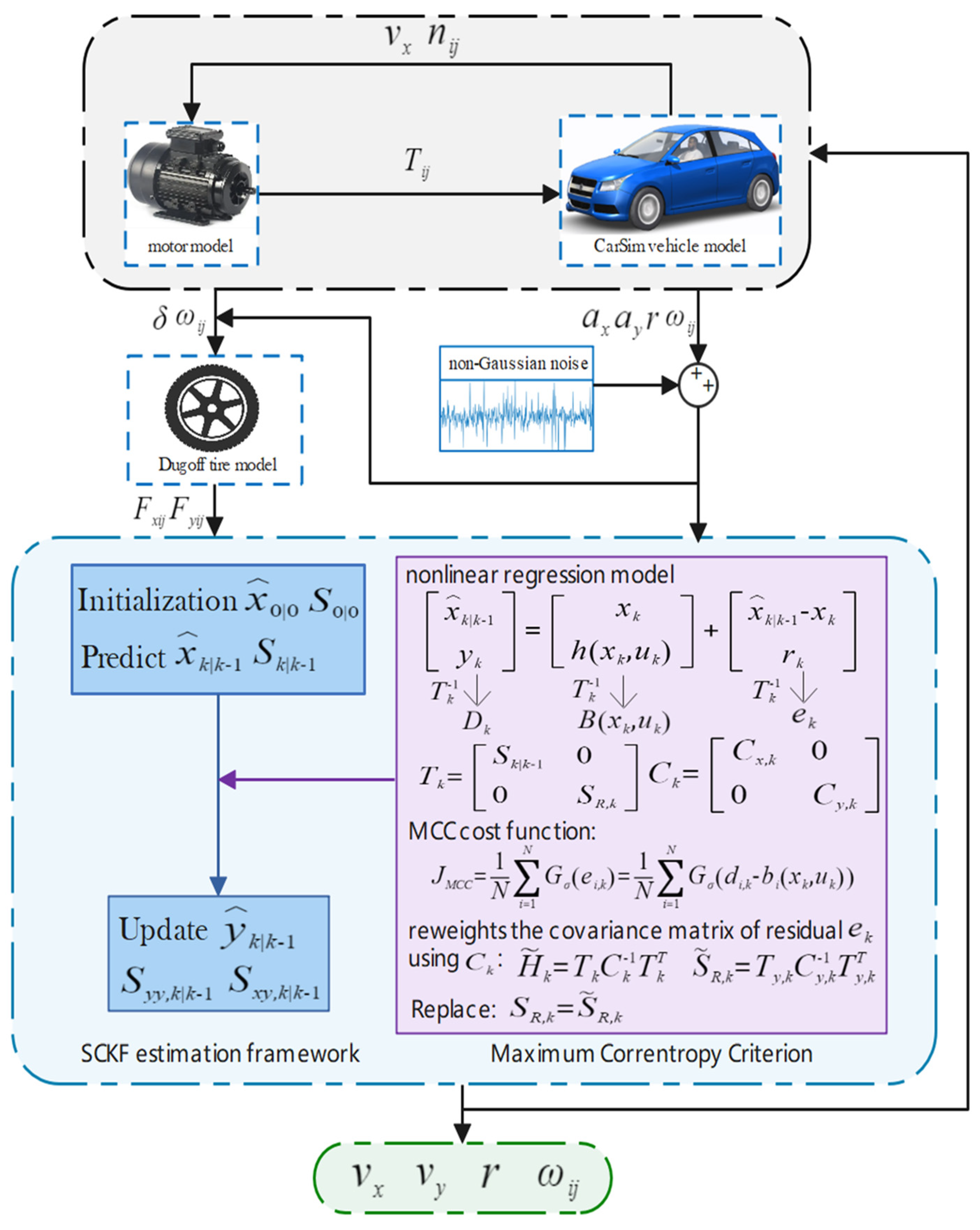
The technical flowchart of estimating vehicle state using the MCSRCKF algorithm is illustrated in Figure 2. The motor model that outputs the desired motor torque T i j based on the desired vehicle speed v x and rotational speed n i j and the on-board sensors on the simulated vehicle measure the steering wheel angle δ , the acceleration a x and a y , the traverse angular velocity r , and the wheel speed ω i j . Then we add non-Gaussian noise to the sensor signals according to the research background of this paper and also provide it to the Dugoff tire model to estimate the tire force. Finally, the sensor measurement signal is substituted into the MCSRCKF algorithm flow as y k , and then the measurement noise can be updated in real-time using the MCSRCKF.
Finally, estimation results from the CKF, SCKF, and MCSRCKF were respectively compared for the double-lane change condition and the serpentine condition with the same input variables and vehicle model. Set the parameters for the simulated vehicle in Table 2.
Before the simulation experiment, the initial values for process noise and measurement noise in the estimator need to be continuously adjusted through extensive simulation experiments because the covariance matrix of the algorithm in the observer and the sensor noise characteristics are closely related. In real vehicle operation, the sensor noise is considered non-Gaussian, particularly heavy-tailed noise with large outliers, because large outliers frequently cause the measurement signal to be disturbed. In this paper, it is assumed that the process noise and the measurement noise both consist of heavy-tailed non-Gaussian noise. In order to more closely approach the situation where the measurement effect of the sensor is greatly affected at high speed, select low-cost and low-accuracy sensors installed on distributed drive vehicles and set up large measurement noise. Therefore, the covariance matrix is as follows:
Set the system noise and observation noise to:
q i ~ 0.8 N 0 , 0.001 + 0.2 N 0 , 0.1
r i ~ 0.8 N 0 , 10 + 0.2 N 0 , 1000
where, i = 1 , 2 , , 7 , representing system noise and observation noise respectively.

4.2. Experimental Results and Analysis

In both the double-lane change condition and the snaking condition, the vehicle system’s driving state changed drastically, and both working conditions adequately validated that the proposed method is effective. Comparing the MCSRCKF used on this paper with the conventional CKF and the SRCKF improved by RQ decomposition under the same operating conditions and the root mean square error (RMSE) index to evaluate the estimated accuracy by different methods with the following equation:
R M S E = 1 M k = 1 M x ^ k x k 2
RMSE is more sensitive to the overall error; for example, in the double-lane change condition, RMSE will amplify the large errors, making differences between algorithms more obvious. However, there are more large outliers in the serpentine condition; in this case, using the mean absolute error (MAE) index to analyze the estimated performance, which only considers absolute errors, is more robust. Its calculation formula is shown as follows:
M A E = 1 M i = 1 M x ^ k x k
where k is the current moment and M is the amount of sampling points.

4.2.1. Double-Lane Change Condition

Simulations are performed at an initial vehicle velocity of 90 km/h on a structured pavement, and the adhesion coefficient is set to 0.85. Equations (58) to (59) denote the initial values for the system noise, and the equations shown below express the initial state vector values with their corresponding covariance matrices:
x 0 = 90 / 3.6 , 0 , 0 , 90 / 3.6 / R 0 , 90 / 3.6 / R 0 , 90 / 3.6 / R 0 , 90 / 3.6 / R 0
P = d i a g 0.01 , 0.01 , 0.01 , 0.01 , 0.01 , 0.01 , 0.01
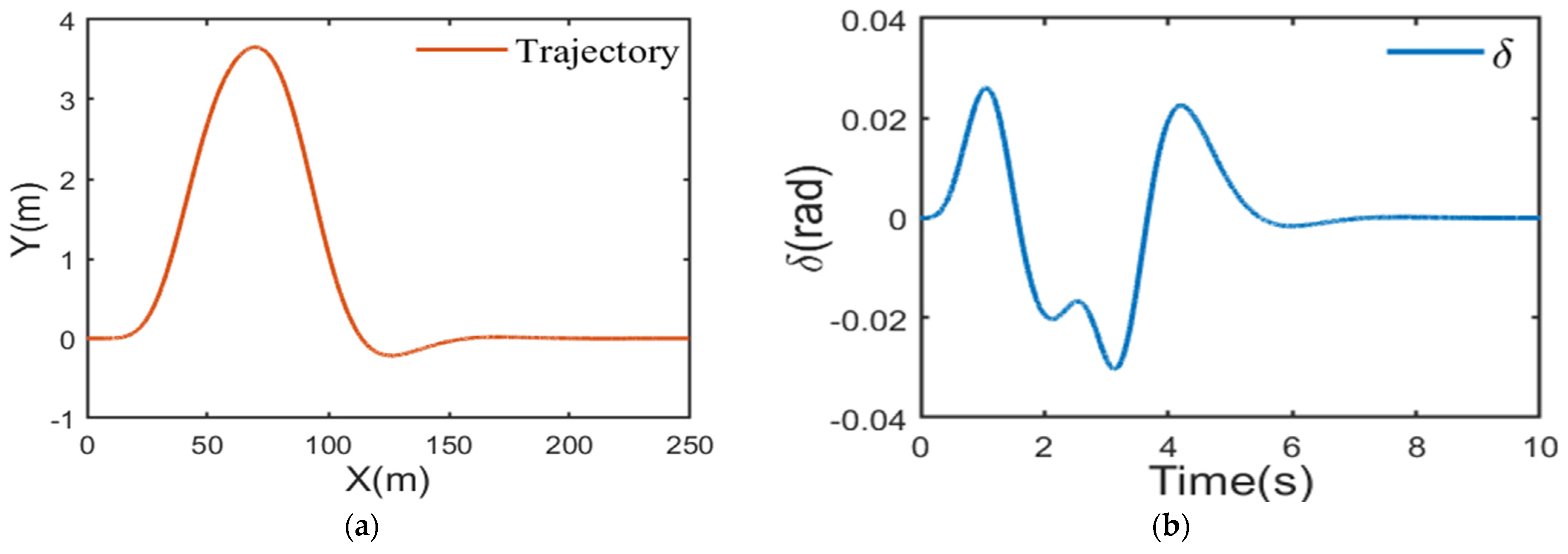
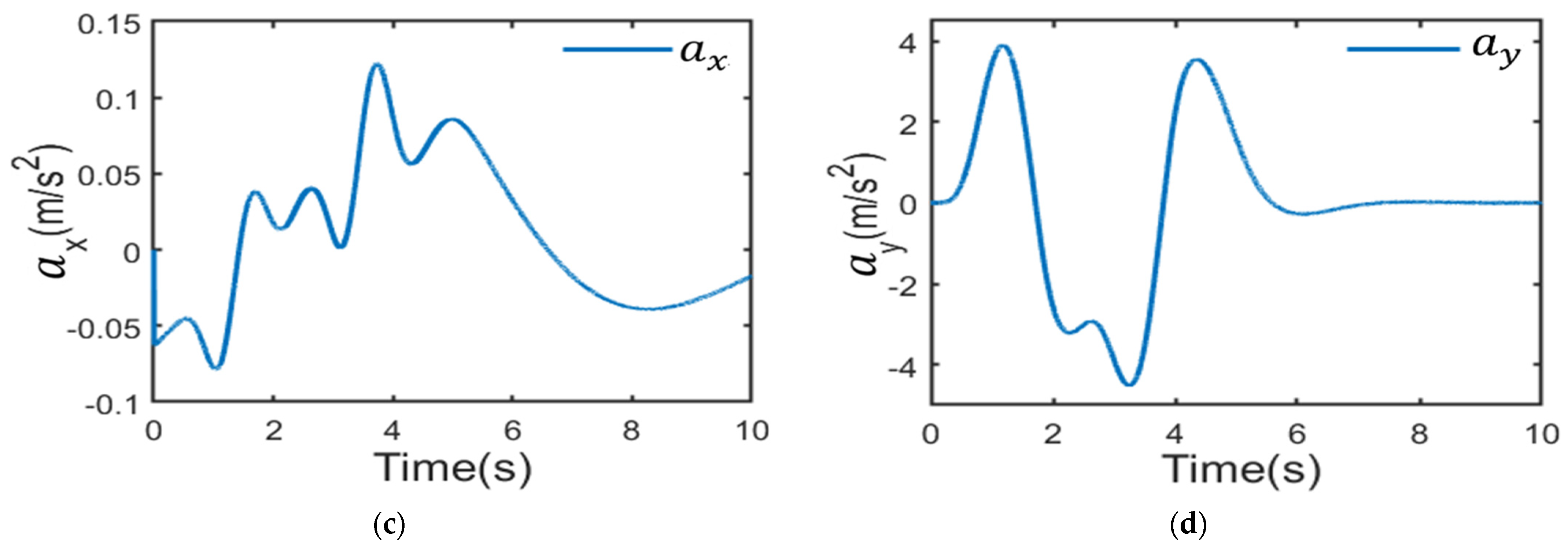
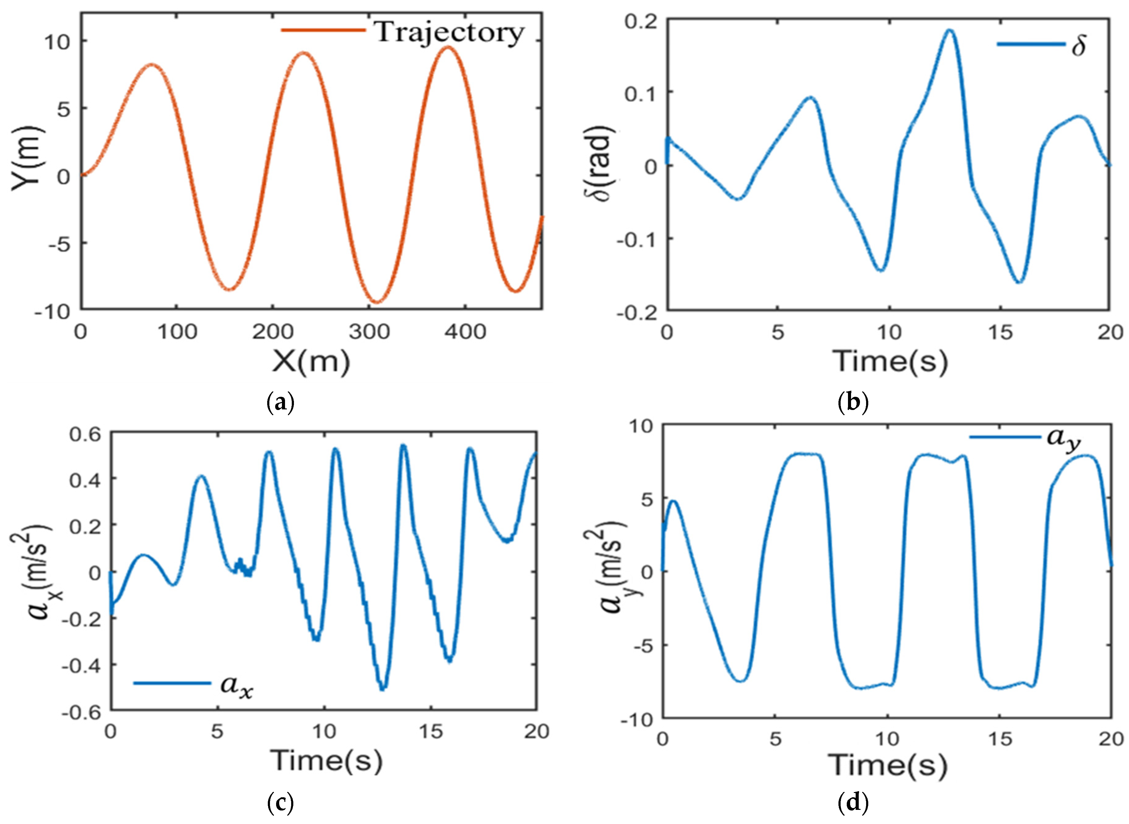
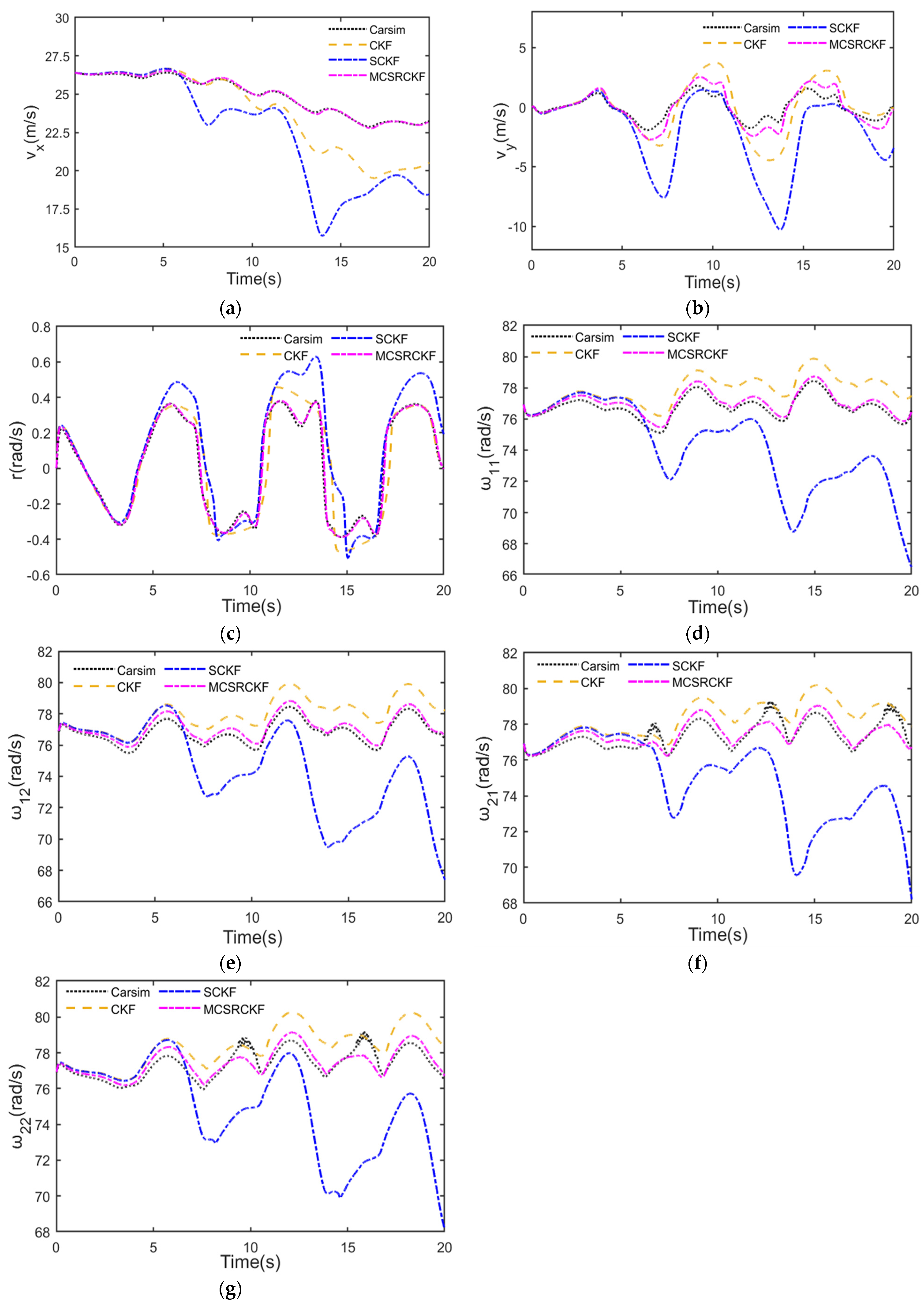
The driving trajectory, input signals, and observed signals for the estimator are given in Figure 3, and Figure 4 compares the simulation data of the CKF, SCKF, and MCSRCKF in estimating the vehicle state.
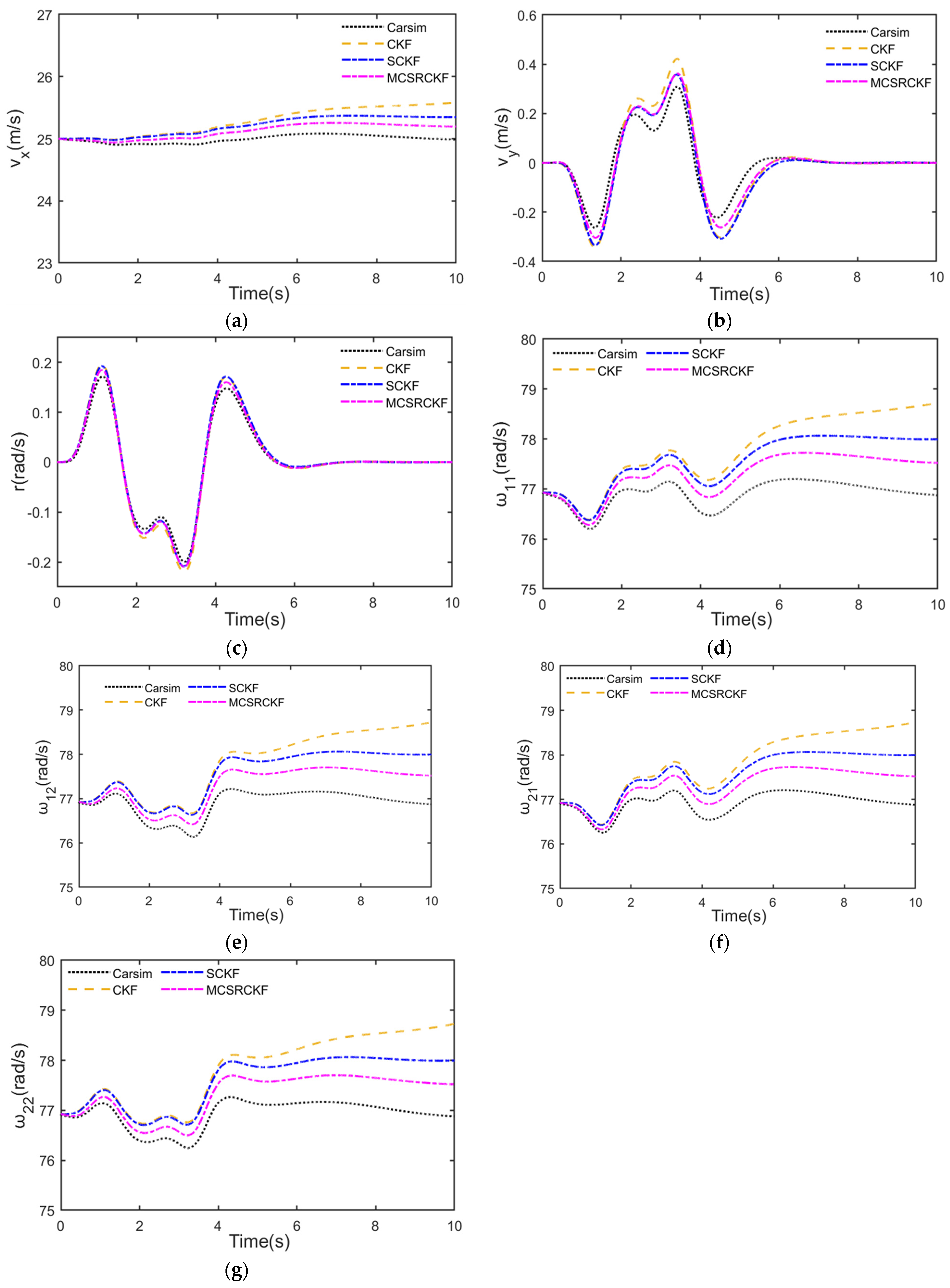
From Figure 4a, it can be observed that the longitudinal speed estimation of the SCKF is better than that of the CKF for this condition, which is because the QR decomposition used by the SCKF replaces the Cholesky decomposition and suppresses the filtering divergence problem arising from the non-positive timing of the covariance matrix. From Table 3, it can be seen that the RMSE of the SCKF is to some extent reduced compared to the CKF, and the RMSE of the MCSRCKF is further reduced compared with the former two. Comparing with the SCKF, the vehicle speed in the longitudinal and lateral directions, respectively, decreased 40.8% and 20.2%, the yaw rate decreased 34%, and the estimated curve of the MCSRCKF is closest to the true value. The reason is that the algorithm uses the discrepancy between the sensor measurements and the true values to construct the MCC’s cost function and calculate the matrix of measurement error when the measured value has the strongest correlation with the real value, achieving a real-time update of measurement noise. Therefore, compared with CKF and SCKF, which set the noise to a constant value, MCSRCKF is more adapted to estimate the driving state of distributed drive vehicles in a strongly nonlinear non-Gaussian noise environment by estimating the current measurement noise in real time.
From Figure 4b lateral speed, Figure 4c yaw rate, and Figure 4d–g four wheel rotational angular speed, it can also be seen that the yaw rate changes sharply when the vehicle turns and changes lanes at high speed, and there is a high risk of outliers in the measured data. The noise near the outliers presents a heavy-tailed characteristic, which leads to large errors in the CKF and SCKF at the peak. At this time, MCSRCKF can deal with the influence of discrete points on the estimator and make the results more convergent to the true value, which has strong robustness.

4.2.2. Serpentine Condition

For more comprehensive verification of the algorithm’s adaptive capability, in the strong nonlinear limit condition, select the serpentine condition of continuous turning with an adhesion coefficient of 0.85 and the initial vehicle driving speed set to 95 km/h. Equations (58) and (59) express the initial process noise and the measurement noise, and the equations shown below express the initial state vector values with their corresponding covariance matrices:
x 0 = 95 / 3.6 , 0 , 0 , 95 / 3.6 / R 0 , 95 / 3.6 / R 0 , 95 / 3.6 / R 0 , 95 / 3.6 / R 0
P = d i a g 0.01 , 0.01 , 0.01 , 0.01 , 0.01 , 0.01 , 0.01
The driving trajectory, import, and observed signals of the estimator are described in Figure 5, and the simulation results of estimating the driving state for distributed drive vehicles by the CKF, SCKF, and MCSRCKF are compared in Figure 6.
In the serpentine condition, the simulation result curves of longitudinal speed, lateral speed, and yaw rate are respectively compared in Figure 6a–c. As is clear from the figures, the CKF and SCKF follow the true values poorly because the vehicle system in continuous turning at high speed exhibits strong nonlinear characteristics in the dramatically changing driving environment, and the measurement accuracy of the on-board sensors is reduced, which is prone to generating outlier data, resulting in large errors at the peak. In particular, the SCKF is heavily contaminated by non-Gaussian noise, and the estimation performance deteriorates sharply, with large fluctuations and gradual dispersion in the filtering results at the 6th second.
From Table 4, the RMSE of the lateral speed estimates obtained by the SCKF reaches 3.36, the average absolute error of the MCSRCKF in longitudinal speed estimation is 95.1% lower than that of the CKF, and the lateral speed and yaw rate decreased by 55.6% and 81.3%, respectively. And the simulation results of MCSRCKF basically match with the real value curve, which can maintain tracking consistency even when the vehicle makes continuous turning operations and only has small fluctuations near the true value, which can rapidly and accurately convert to the true value, showing the highest estimation accuracy, the strongest robustness, and the best real-time performance. Compared with the double-shift condition, the improvement in the estimation accuracy of MCSRCKF in the serpentine condition is greater. Therefore, we can conclude that the MCSRCKF is better in the strong nonlinear limit condition with large deviations and exhibits more powerful convergence ability.

5. Conclusions

In this paper, we adopt MCSRCKF, which has solved the driving state estimation problems for distributed nonlinear vehicles in a non-Gaussian noise environment. After comparing and analyzing the results of simulated experiments in the Double-lane change condition and serpentine condition at high speed, it is demonstrated that this algorithm is accurate in estimating the driving state of the nonlinear vehicle system under a heavy-tailed non-Gaussian noise influence. Firstly, an electric vehicle model with distributed driving is built by combining a 7-DOF vehicle dynamic model, an electric motor model, and the Dugoff tire model. Secondly, the vehicle’s longitudinal speed, lateral speed, yaw rate, and four-wheel rotation speed are accurately observed on the basis of the MCSRCKF algorithm, and the estimated values at each moment are fed back to the vehicle model for the next moment of calculation, forming a closed-loop system through mutual exchange of information and mutual correction. Analyzing the experimental data obtained from the simulation, from the values of RMSE and MAE, it can be clearly seen that the estimation error of MCSRCKF has been reduced significantly compared to both CKF and SCKF, and from the simulation curve, it can be seen that the estimation result of MCSRCKF at the peak of the curve is more closely fit to the real value, especially in the limiting conditions, because MCC reduces the influence of the outliers in the non-Gaussian noise environment on the estimation accuracy. We can sufficiently confirm that the MCSRCKF performs well in noise immunity, can better estimate the longitudinal, lateral, and yaw, can maintain small fluctuations in extreme working conditions, has strong robustness, and ultimately converges to its value by providing real-time and accurate information of key vehicle parameters for the control system, which provides high applied value for the development of intelligent vehicles.
In the subsequent research, we will attempt to apply the method to real vehicle tests and consider more dimensions of vehicle motion to obtain further improvements in estimation accuracy and real-time performance.

Author Contributions

Conceptualization, P.G. and C.Z.; methodology, C.Z.; software, T.Z. and L.G.; validation, P.G. and Q.X.; resources, P.G.; writing—original draft preparation, C.Z. and Q.X.; writing—review and editing, P.G.; funding acquisition, P.G. and L.G. All authors have read and agreed to the published version of the manuscript.

Funding

This research was supported by the National Natural Science Foundation of China, grant numbers 52175078 and 51975089, and the Fundamental Research Funds for the Central Universities, grant number DUT22QN248, and the National Key Research and Development Program of China, grant number 2022YFB2602305.

Institutional Review Board Statement

Not applicable.

Informed Consent Statement

Not applicable.

Data Availability Statement

Not applicable.

Conflicts of Interest

The authors declare no conflict of interest.

References

  1. Ahangarnejad, A.H.; Radmehr, A.; Ahmadian, M. A review of vehicle active safety control methods: From antilock brakes to semiautonomy. J. Vib. Control 2021, 27, 1683–1712. [Google Scholar] [CrossRef]
  2. Zhuang, Y.; Sun, X.; Li, Y. Multi-sensor integrated navigation/positioning systems using data fusion: From analytics-based to learning-based approaches. Inf. Fusion 2023, 95, 62–90. [Google Scholar]
  3. Xia, X.; Xiong, L.; Huang, Y. Estimation on IMU yaw misalignment by fusing information of automotive onboard sensors. Mech. Syst. Signal Process. 2022, 162, 107993. [Google Scholar] [CrossRef]
  4. Marco, V.R.; Kalkkuhl, J.; Raisch, J. Multi-modal sensor fusion for highly accurate vehicle motion state estimation. Control Eng. Pract. 2020, 100, 104409. [Google Scholar] [CrossRef]
  5. Hu, J.Y.; Wang, Y.; Yan, Y.J.; Di, K.K.; Bai, S.; Yin, G.D. Vehicle state estimation based on limited memory random weighted extended Kalman filter. J. Southeast Univ. 2022, 2, 387–393. [Google Scholar]
  6. Julier, S.J.; Uhlmann, J.K. New extension of the Kalman filter to nonlinear systems. Signal processing, sensor fusion, and target recognition VI. SPIE 1997, 3068, 182–193. [Google Scholar]
  7. Wan, W.; Feng, J.; Song, B.; Li, X. Huber-Based Robust Unscented Kalman Filter Distributed Drive Electric Vehicle State Observation. Energies 2021, 14, 750. [Google Scholar] [CrossRef]
  8. Wu, Y.; Hu, D.; Wu, M. A numerical-integration perspective on Gaussian filters. IEEE Trans. Signal Process. 2006, 54, 2910–2921. [Google Scholar] [CrossRef]
  9. Arasaratnam, I.; Haykin, S. Cubature kalman filters. IEEE Trans. Autom. Control 2009, 54, 1254–1269. [Google Scholar] [CrossRef] [Green Version]
  10. Li, Y.; Li, J.; Qi, J. Robust cubature Kalman filter for dynamic state estimation of synchronous machines under unknown measurement noise statistics. IEEE Access 2019, 7, 29139–29148. [Google Scholar] [CrossRef]
  11. Wan, W.; Jingan, F.; Bao, S.; Xinxin, L. Vehicle state estimation using interacting multiple model based on square root cubature Kalman filter. Appl. Sci. 2021, 11, 10772. [Google Scholar]
  12. Wu, Y.; Li, G.; Fan, D. Joint estimation of driving state and road adhesion coefficient for distributed drive electric vehicle. IEEE Access 2021, 9, 75460–75469. [Google Scholar] [CrossRef]
  13. Boufadene, M.; Belkheiri, M.; Rabhi, A. Vehicle longitudinal force estimation using adaptive neural network nonlinear observer. Int. J. Veh. Des. 2019, 79, 205–220. [Google Scholar] [CrossRef]
  14. Jie, C.; Cheng, L.; Ming-Gang, G.A.N. Extension of SGMF using Gaussian sum approximation for nonlinear/non-Gaussian model and its application in multipath estimation. Acta Autom. Sin. 2013, 39, 1–10. [Google Scholar]
  15. Kaczmarek, K.; Domański, P.D. Study on outlier robustness of minimum variance control performance assessment. Int. J. Adapt. Control Signal Process. 2021, 35, 2175–2193. [Google Scholar] [CrossRef]
  16. Liu, X.; Ren, Z.; Lyu, H. Linear and nonlinear regression-based maximum correntropy extended Kalman filtering. IEEE Trans. Syst. Man Cybern. Syst. 2019, 51, 3093–3102. [Google Scholar] [CrossRef]
  17. Liu, D.; Chen, X.; Xu, Y. Maximum correntropy generalized high-degree cubature Kalman filter with application to the attitude determination system of missile. Aerosp. Sci. Technol. 2019, 95, 105441. [Google Scholar] [CrossRef]
  18. Li, M.; Tang, X.; Zhang, Q. Non-Gaussian Pseudolinear Kalman Filtering-Based Target Motion Analysis with State Constraints. Appl. Sci. 2022, 12, 9975. [Google Scholar] [CrossRef]
  19. Huang, Y.; Zhang, Y.; Zhao, Y. A novel robust Gaussian–Student’s t mixture distribution based Kalman filter. IEEE Trans. Signal Process. 2019, 67, 3606–3620. [Google Scholar] [CrossRef]
  20. Shi, Q.; Liu, M.; Hang, L. A novel distribution system state estimator based on robust cubature particle filter used for non-gaussian noise and bad data scenarios. IET Gener. Transm. Distrib. 2022, 16, 1385–1399. [Google Scholar] [CrossRef]
  21. Zhang, Q. Performance enhanced Kalman filter design for non-Gaussian stochastic systems with data-based minimum entropy optimisation. AIMS Electron. Electr. Eng. 2019, 3, 382–396. [Google Scholar] [CrossRef]
  22. Chen, B.; Dang, L.; Gu, Y. Minimum error entropy Kalman filter. IEEE Trans. Syst. Man Cybern. Syst. 2019, 51, 5819–5829. [Google Scholar] [CrossRef] [Green Version]
  23. He, J.; Wang, G.; Yu, H. Generalized minimum error entropy Kalman filter for non-Gaussian noise. ISA Trans. 2022, 136, 663–675. [Google Scholar] [CrossRef] [PubMed]
  24. Fan, X.; Wang, G.; Han, J. Interacting multiple model based on maximum correntropy Kalman filter. IEEE Trans. Circuits Syst. II Express Briefs 2021, 68, 3017–3021. [Google Scholar] [CrossRef]
  25. Wang, J.; Lyu, D.; He, Z. Cauchy kernel-based maximum correntropy Kalman filter. Int. J. Syst. Sci. 2020, 51, 3523–3538. [Google Scholar] [CrossRef]
  26. Liu, C.; Wang, G.; Guan, X. Robust M-estimation-based maximum correntropy Kalman filter. ISA Trans. 2022, 136, 198–209. [Google Scholar] [CrossRef]
  27. Saha, J.; Bhaumik, S. Robust Maximum Correntropy Kalman Filter. arXiv 2023, arXiv:2302.02694. [Google Scholar]
  28. Chen, B.; Liu, X.; Zhao, H. Maximum correntropy Kalman filter. Automatica 2017, 76, 70–77. [Google Scholar] [CrossRef] [Green Version]
  29. Izanloo, R.; Fakoorian, S.A.; Yazdi, H.S. Kalman filtering based on the maximum correntropy criterion in the presence of non-Gaussian noise. In Proceedings of the 2016 Annual Conference on Information Science and Systems (CISS), Princeton, NJ, USA, 16–18 March 2016; IEEE: Piscataway, NJ, USA; pp. 500–505. [Google Scholar]
  30. Mohiuddin, S.M.; Qi, J. Maximum correntropy extended Kalman filtering for power system dynamic state estimation. In Proceedings of the IEEE Power & Energy Society General Meeting (PESGM), Atlanta, GA, USA, 4–9 August 2019; IEEE: Piscataway, NJ, USA; pp. 1–5. [Google Scholar]
  31. Ma, F.; Liu, F.; Zhang, X. An ultrasonic positioning algorithm based on maximum correntropy criterion extended Kalman filter weighted centroid. Signal Image Video Process 2018, 12, 1207–1215. [Google Scholar] [CrossRef]
  32. Wang, G.; Zhang, Y.; Wang, X. Iterated maximum correntropy unscented Kalman filters for non-Gaussian systems. Signal Process 2019, 163, 87–94. [Google Scholar] [CrossRef]
  33. Arasaratnam, I. Cubature Kalman Filtering Theory & Applications. Ph.D. Thesis, McMaster University, Hamilton, ON, Canada, 2009. [Google Scholar]
  34. Zhang, J.; Jian, J.; Dong, K. Volume filtering algorithm based on maximum correlation entropy criterion under noise non-Gaussian conditions. J. Ordnance Equip. Eng. 2021, 42, 245–250. [Google Scholar]
  35. Li, S.; Xu, B.; Wang, L. Improved maximum correntropy cubature Kalman filter for cooperative localization. IEEE Sens. J. 2020, 20, 13585–13595. [Google Scholar] [CrossRef]
  36. Xia, D.; Liu, Q.; Lu, D. Friction Prediction and Application to Lateral or Longitudinal Slip Force Prediction. Machines 2022, 10, 791. [Google Scholar] [CrossRef]
  37. Feng, Y.; Huang, X.; Shi, L. Learning with the maximum correntropy criterion induced losses for regression. J. Mach. Learn. Res. 2015, 16, 993–1034. [Google Scholar]
  38. Hou, B.; He, Z.; Li, D.; Zhou, H.; Wang, J. Maximum Correntropy Unscented Kalman Filter for Ballistic Missile Navigation System based on SINS/CNS Deeply Integrated Mode. Sensors 2018, 18, 1724. [Google Scholar] [CrossRef] [PubMed] [Green Version]
  39. Zhang, Z.; Hao, Y.; Wu, X. Complexity analysis of three deterministic sampling nonlinear filtering algorithms. J. Harbin Inst. Technol. 2013, 45, 111–115. [Google Scholar]
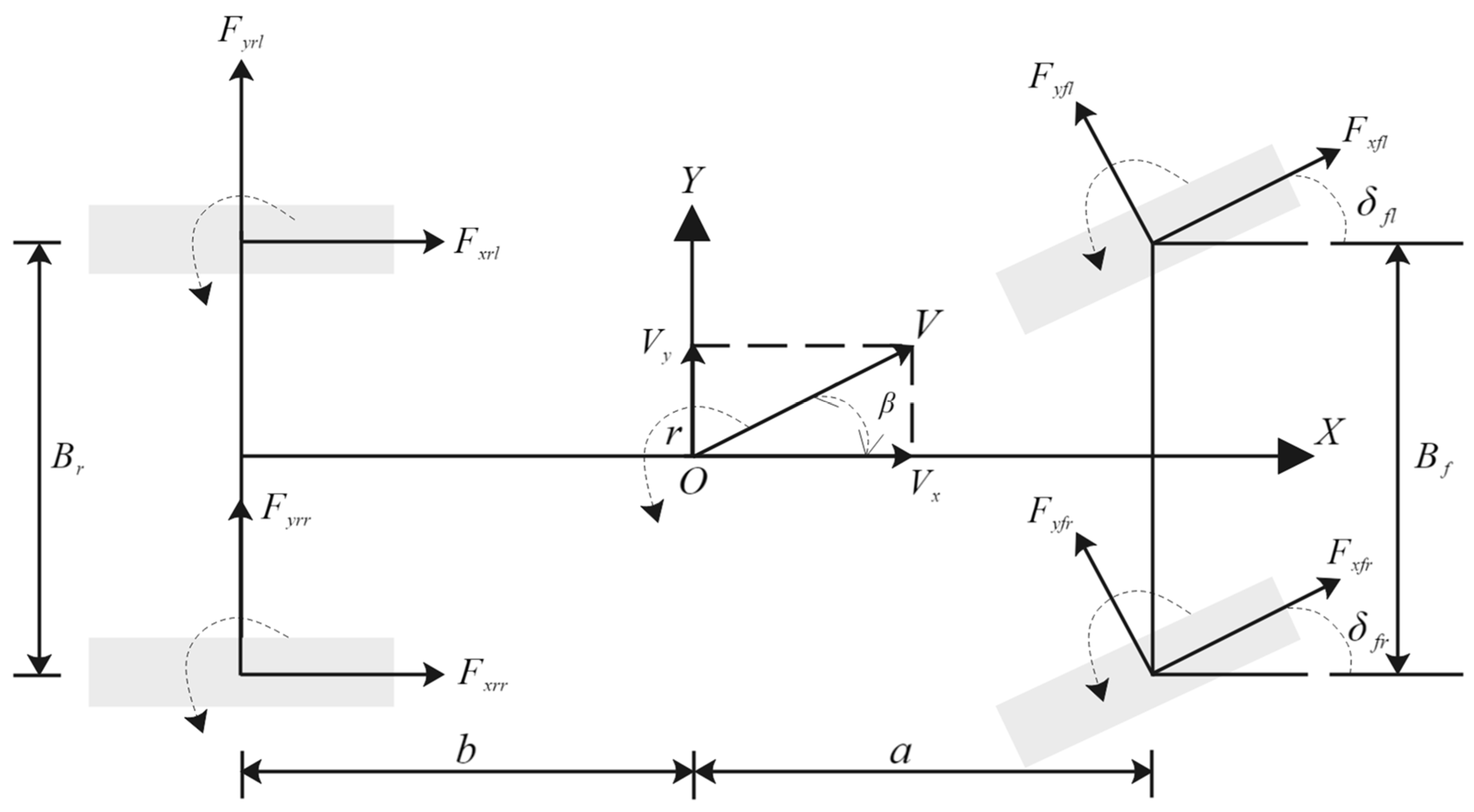
Figure 1. 7-DOF vehicle dynamics model.
Applsci 13 08762 g001
Figure 2. MCSRCKF flow chart.
Applsci 13 08762 g002
Figure 3. Double-lane change condition: (a) Driving trajectory of vehicle; (b) front wheel angle; (c) longitudinal acceleration; (d) lateral acceleration.
Applsci 13 08762 g003aApplsci 13 08762 g003b
Figure 4. Simulated vehicle state results in case of the Double-lane change condition: (a) longitudinal speed; (b) lateral speed; (c) yaw rate; (d) Rotation speed of left front wheel; (e) Rotation speed of right front wheel; (f) Rotation speed of left rear wheel; (g) Rotation speed of right rear wheel.
Applsci 13 08762 g004
Figure 5. Serpentine condition: (a) vehicle driving trajectory; (b) front wheel angle; (c) longitudinal acceleration; (d) lateral acceleration.
Applsci 13 08762 g005
Figure 6. Simulated vehicle state results in case of the serpentine condition: (a) longitudinal speed; (b) lateral speed; (c) yaw rate; (d) Rotation speed of left front wheel; (e) Rotation speed of right front wheel; (f) Rotation speed of left rear wheel; (g) Rotation speed of right rear wheel.
Applsci 13 08762 g006
Table 1. The computational complexity of some Equation, where n and m denote the dimensions of the state and measurement vectors, respectively.
EquationAddition/Subtraction, Multiplication, Matrix Inversion, Cholesky Decomposition, and QR Decomposition EquationAddition/Subtraction, Multiplication, Matrix Inversion, Cholesky Decomposition, and QR Decomposition
(23) 1 3 n 3 (32) 2 3 m 3
(24) 4 n 3 (33) 2 n m + 1 3 m 3
(25) 4 n 3 2 n 2 (34) 2 n 2 + 4 n 2 m n m
(26) 2 n 2 (36) 2 m 3 + 4 n m 2 2 n m
(27) 2 3 n 3 (37) 2 n m + m
(28) 2 n 2 + 1 3 n 3 (38) 2 3 n 3 + 4 n 2 m + 2 n m 2 n m + 1 3 m 3
(29) 4 n 3 (45) ( n + m ) 3 + 4 ( n + m ) 2 2 ( n + m )
(30) 4 n 2 m 2 n m (54) 5 m 3 2 m 2
(31) 2 n m
Table 2. Parameter configuration of the simulation vehicle.
Vehicle Parameter NameSymbolValue
Vehicle mass m 1418 kg
Distance between the front axle and the mass center a 1.016 m
Distance between the rear axle and the mass center b 1.896 m
Wheelbase of front wheels T f 1.675 m
Wheelbase of rear wheels T r 1.675 m
Yaw moment of inertia I z 1536 kg·m2
Wheel rolling radius R 0 0.325 m
Centroid height h g 0.54 m
Maximum motor power P m a x 68 kw
Maximum motor torque T m a x 140 N·m
Table 3. MAE and RMSE of various algorithms under the Double-lane change condition.
IndexParametersCKFSCKFMCSCKF
MAE v x ( m / s ) 0.29110.21280.1247
v y ( m / s ) 0.03960.03270.0262
r ( r a d / s ) 0.00750.00630.0041
RMSE v x ( m / s ) 0.33710.23750.1407
v y ( m / s ) 0.05720.04860.0388
r ( r a d / s ) 0.01130.00940.0062
Table 4. MAE and RMSE of various algorithms under the serpentine condition.
IndexParametersCKFSCKFMCSCKF
MAE v x ( m / s ) 1.23432.41480.0605
v y ( m / s ) 1.05602.06440.4690
r ( r a d / s ) 0.06890.11210.0129
RMSE v x ( m / s ) 1.75823.36010.0740
v y ( m / s ) 1.49143.36010.5911
r ( r a d / s ) 0.11140.15240.0209
Disclaimer/Publisher’s Note: The statements, opinions and data contained in all publications are solely those of the individual author(s) and contributor(s) and not of MDPI and/or the editor(s). MDPI and/or the editor(s) disclaim responsibility for any injury to people or property resulting from any ideas, methods, instructions or products referred to in the content.