Research on a Coal Seam Gas Content Prediction Method Based on an Improved Extreme Learning Machine

Abstract

With the rapid advancement of artificial neural network (ANN) algorithms, many researchers have applied these methods to mine gas prediction and achieved numerous research achievements. It is of great significance to study methods that can accurately predict the gas content for the prevention of gas disasters in mining areas. In order to enhance the accuracy, stability, and generalization capability of the gas content prediction model, the GASA-KELM prediction model was established using the GASA algorithm to improve the KELM initial parameter assignment method, and the prediction model based on BPNN and SVM was established under the same conditions. The experimental results show that the GASA-BPNN model failed to achieve the desired outcome within 800 iterations. On the other hand, the GASA-SVM and GASA-KELM models accomplished the goal in significantly fewer iterations, taking only 673 and 487 iterations, respectively. Moreover, the overall average relative errors of the cross-validated gas content predictions were 15.74%, 13.85%, and 9.87% for the three models, respectively. Furthermore, the total average variance of the test set was 3.99, 2.76, and 2.05 for the GASA-BPNN, GASA-SVM, and GASA-KELM models, respectively. As a result, compared with other ANN models, the GASA-KELM model demonstrates higher accuracy, stronger prediction stability, and generalization ability in the practical application. This novel model provides a basis for accurately predicting gas content and proposing effective regional gas management measures.

1. Introduction

Coal resources play a crucial role as an energy source in China and have contributed immensely to the country’s economic development [1,2], and given China’s current energy structure, coal is expected to maintain its dominant position in the energy supply for the foreseeable future [3]. Based on statistics from the National Bureau of Statistics, China is endowed with abundant coal resources, with proven coal reserves of 249.23 billion tons. Additionally, China holds the position of the world’s largest producer and consumer of coal. In 2021, the total primary energy production in China was recorded at 4.33 billion tons of standard coal, with coal accounting for 67% of the overall energy structure. The total energy consumption was 5.24 billion tons of standard coal, with coal consumption contributing to 56.0% of the total primary energy consumption. Ensuring the healthy, stable, and sustainable development of the coal industry is crucial to maintaining the country’s energy security [4]. However, significant disparities in coal resource endowments, complex geological conditions, and deep burial depths across different regions pose substantial obstacles to achieving this goal. China’s robust demand for coal has resulted in an increase in coal mining depths, and mining operations now face high gas pressure, elevated ground stress, and heightened gas content, posing significant threats to mine safety. Although the number of gas accidents has decreased significantly in recent years, the number of fatalities remains high compared to other nations. The issue of mine gas is a major problem that restricts the capacity of coal production, affects the safety of workers, and impedes the economic benefits of coal mines [5,6]. The unclear distribution pattern and occurrence status of CBM, as well as the failure to implement effective gas prevention and control measures, are the primary causes of most gas accidents. Coal seam gas extraction is not only a source of clean and natural energy but also a means to address the pressing issue of gas control [7]. Undoubtedly, methane, a crucial element of coal mine gas, is a potent greenhouse gas [8]. Its ozone-depleting capacity is sevenfold higher than that of carbon dioxide, and its heat-trapping potential is 25 to 30 times higher than an equivalent volume of carbon dioxide. Hence, it holds immense importance to investigate techniques for predicting coalbed methane content from multiple standpoints, such as mitigating gas calamities and safeguarding human lives and property, exploiting and harnessing clean energy, and conserving the environment.

In recent years, with the rapid advancement of machine learning and intelligent algorithms, novel methods such as artificial neural networks (ANNs), support vector machines (SVMs), and extreme learning machines (ELMs) have presented new avenues for tackling high-dimensional, nonlinear, and complex function optimization problems [9]. Hanbo Zheng et al. utilized the SVM to construct a model for predicting the dissolved gas content in power transformers [10]. Feng Yu et al. developed a short-term natural gas load forecasting model using a back propagation neural network (BPNN) [11]. Jiaxing Xin et al. employed a BPNN to identify the deformation characteristics of ACM oil and gas pipelines [12]. Bohan Cao et al. used the ANN to establish a shallow gas identification model for deep water drilling [13]. Machine learning algorithms have garnered widespread application and have yielded fruitful research outcomes in coal seam gas content prediction, coal and gas outburst prediction, and gas outflow prediction. Lin Haifei et al. utilized particle swarm optimization (PSO) to optimize the initial weights and thresholds of the BPNN to create a PSO-BPNN gas content prediction model. In comparison with the multiple linear regression model and the BPNN model, the PSO-BPNN model demonstrated the highest prediction accuracy [14]. Ma Lei et al. implemented the genetic algorithm (GA) and simulated annealing (SA) algorithms to optimize the BPNN for constructing a GASA-BPNN gas content prediction model. During the application process, the model showed a more robust generalization ability for new samples, faster parameter training speed, and higher prediction accuracy [15]. Yaqin Wu et al. introduced an adaptive learning rate to the BPNN and established the GASA-BPNN coal and gas outburst prediction model, which demonstrated good prediction performance during field applications [16]. Zhang Ruilin et al. proposed a coal and gas outburst potential risk level prediction model that combines fault tree and ANN coupling. By utilizing qualitative and quantitative data to solve the model, they made the relationship between geological factors and gas outburst potential risk more evident [17]. Xie Xuecai et al. utilized an improved fruit fly optimization algorithm (IFOA) to optimize the general regression neural network (GRNN), leading to the development of the IFOA-GRNN model for predicting coal and gas outbursts. The IFOA-GRNN model displays the desirable attributes of low prediction errors, high stability, and rapid convergence speed during practical applications [18]. Qian Meng et al. proposed a coal seam gas content prediction model based on an SVM and PSO. The results of practical applications revealed that the PSO-SVR model outperforms both the ANN model and the ordinary support vector regression (SVR) model, particularly with a limited number of samples [19]. Zhang Sirui et al. improved the grey prediction model by incorporating a BPNN, ultimately establishing an enhanced gas concentration prediction model based on grey theory and the BPNN. The simulation results indicate that this model significantly improves the prediction accuracy of the gas concentration [20]. Zhenhua Yang et al. introduced an improved residual gas content prediction method based on the drilling cutting index and the bat algorithm-optimized ELM. In comparison with the BPNN, SVM, and ELM, this novel method exhibits superior accuracy and effectively uncovers the nonlinear relationship between the drilling cutting index and residual gas content [21]. Liming Qiu et al. established a protrusion risk prediction model based on a convolutional neural network. This model explores the correlation between post-explosion gas concentration changes and coal seam protrusion risks, which is crucial in improving coal and gas outburst prediction accuracy [22]. Xiang Wu et al. proposed a gas outburst prediction model based on the grey relation analysis (GRA) and adaptive PSO algorithm-optimized SVM. Their study demonstrates that the new model exhibits better performance than the SVM and PSO-SVM outburst prediction models [23].

With regard to predicting coalbed methane content, the predominant approach involves leveraging gas geological theory to analyze the factors that influence methane content. By comprehensively considering these factors and employing mathematical techniques to establish a functional mapping relationship between the influencing factors and the target of prediction, accurate predictions can be achieved. The results demonstrate that this method surpasses traditional prediction methods and exhibits a relatively high accuracy rate. To overcome the limitations of ELM, BPNN, and SVM, researchers have integrated intelligent algorithms to optimize their parameters. However, the application of algorithms for parameter optimization is based on a random search algorithm framework, which still has room for improvement in terms of functionality. During the process of developing prediction models, researchers commonly rely on a single algorithm to optimize model parameters. Nevertheless, using a single algorithm may lead to limitations such as being vulnerable to local optima, exhibiting poor generalization ability, and achieving low accuracy when addressing intricate issues. To overcome the limitations of single algorithm optimization, the GASA hybrid optimization algorithm with complementary advantages is designed by using a divide-and-conquer strategy by comprehensively exploiting the differences and complementarities of different intelligent algorithms. The GASA algorithm is used to optimize KELM, SVM and BPNN to build three gas content prediction models to obtain a gas content prediction model with faster iteration speed, higher prediction accuracy, and stronger generalization ability.

2. Development of Prediction Models for Coal Seam Gas Content

2.1. Theoretical Analysis and Performance Evaluation of the GASA Optimization Algorithm

2.1.1. Theoretical Analysis of the GASA Optimization Algorithm

The GA is a stochastic search algorithm that mimics the genetic mechanism of nature and Darwin’s theory of biological evolution [24,25]. The GA uses a coding space to represent the parameter space of the problem and evaluates the fitness of individuals in the population based on a fitness function. This approach simulates biological selection and genetic mechanisms through genetic operations to generate new individuals who outperform the previous generation. Through repeated iterations, the algorithm approaches the global optimum solution. Figure 1 shows the flowchart of the GA algorithm.

The SA algorithm is a random search algorithm that is based on the Monte Carlo iterative solution strategy [26,27]. Its starting point is inspired by the similarity between the annealing process of solid materials and combinatorial optimization problems. The SA algorithm starts with a high initial temperature and applies the Metropolis sampling criterion, which accepts suboptimal solutions in the neighborhood with a certain probability. This allows the algorithm to effectively avoid becoming stuck in local optima in the early stage. In the later stage, the algorithm improves its convergence efficiency by rejecting suboptimal solutions with a high probability. This overcomes the problem of the algorithm becoming easily trapped in local optimal solutions and is crucial to the SA algorithm’s ability to converge globally. The SA algorithm process is depicted in Figure 1.

The GASA algorithm is designed to combine the advantageous features of SA and GA, namely, SA’s gradually decreasing probability jump and GA’s survival of the fittest, to overcome the challenge of becoming trapped in local minima during the search process. Structurally, while GA simultaneously searches the population using the neighborhood function, SA only concentrates on a single individual at a time. The GASA algorithm combines these approaches by executing SA sequentially on each individual in the GA population, diversifying the neighborhood search structure of each individual and enhancing the algorithm’s search capability and efficiency.

The GASA algorithm adheres to the process illustrated in Figure 2. The optimization process can be summarized as follows [16]:

(1)

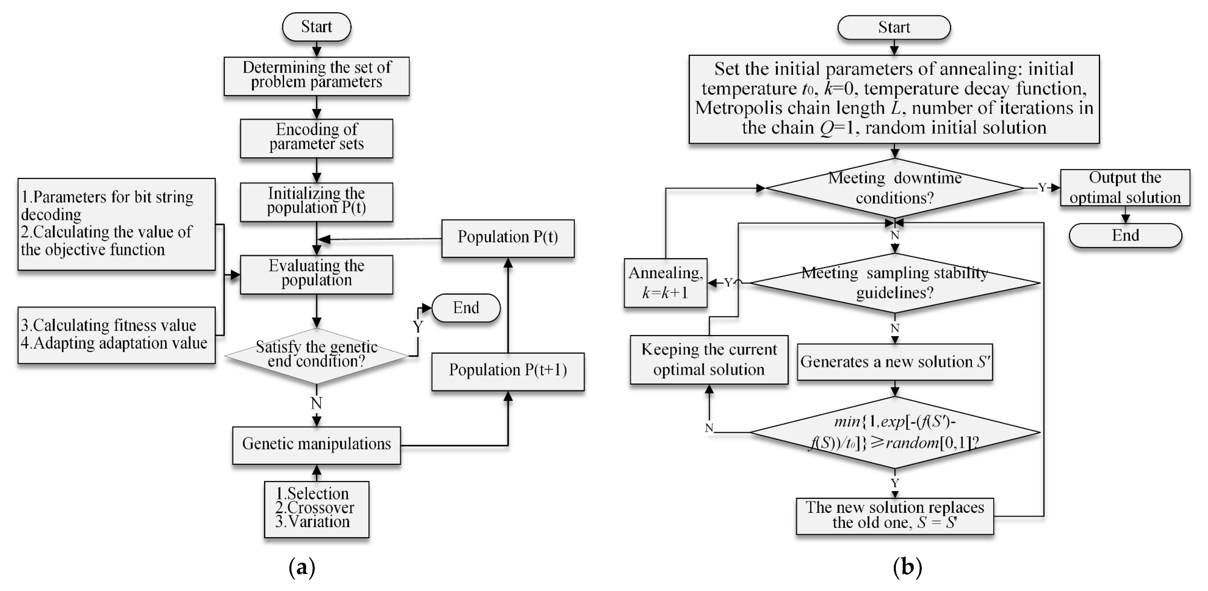
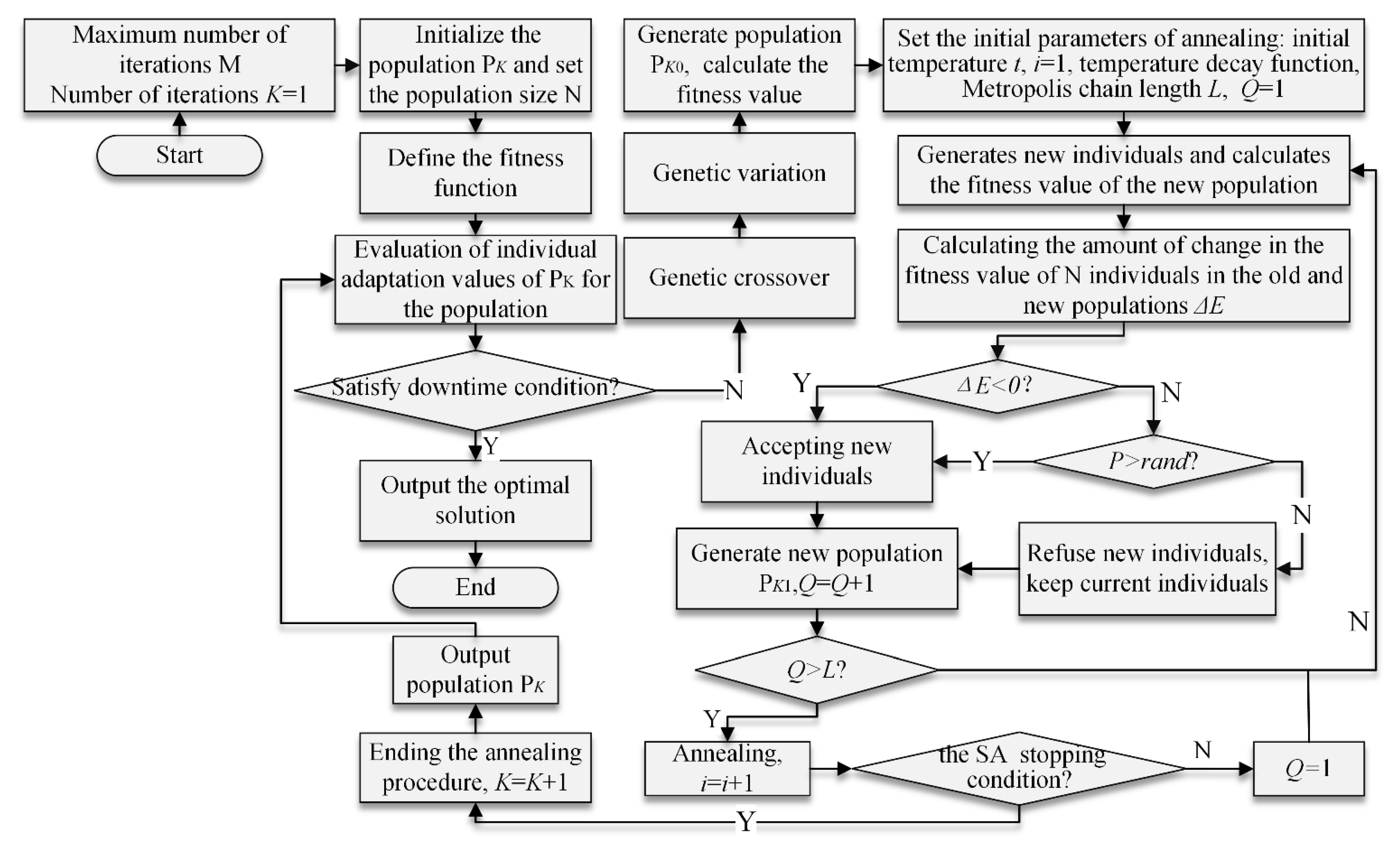
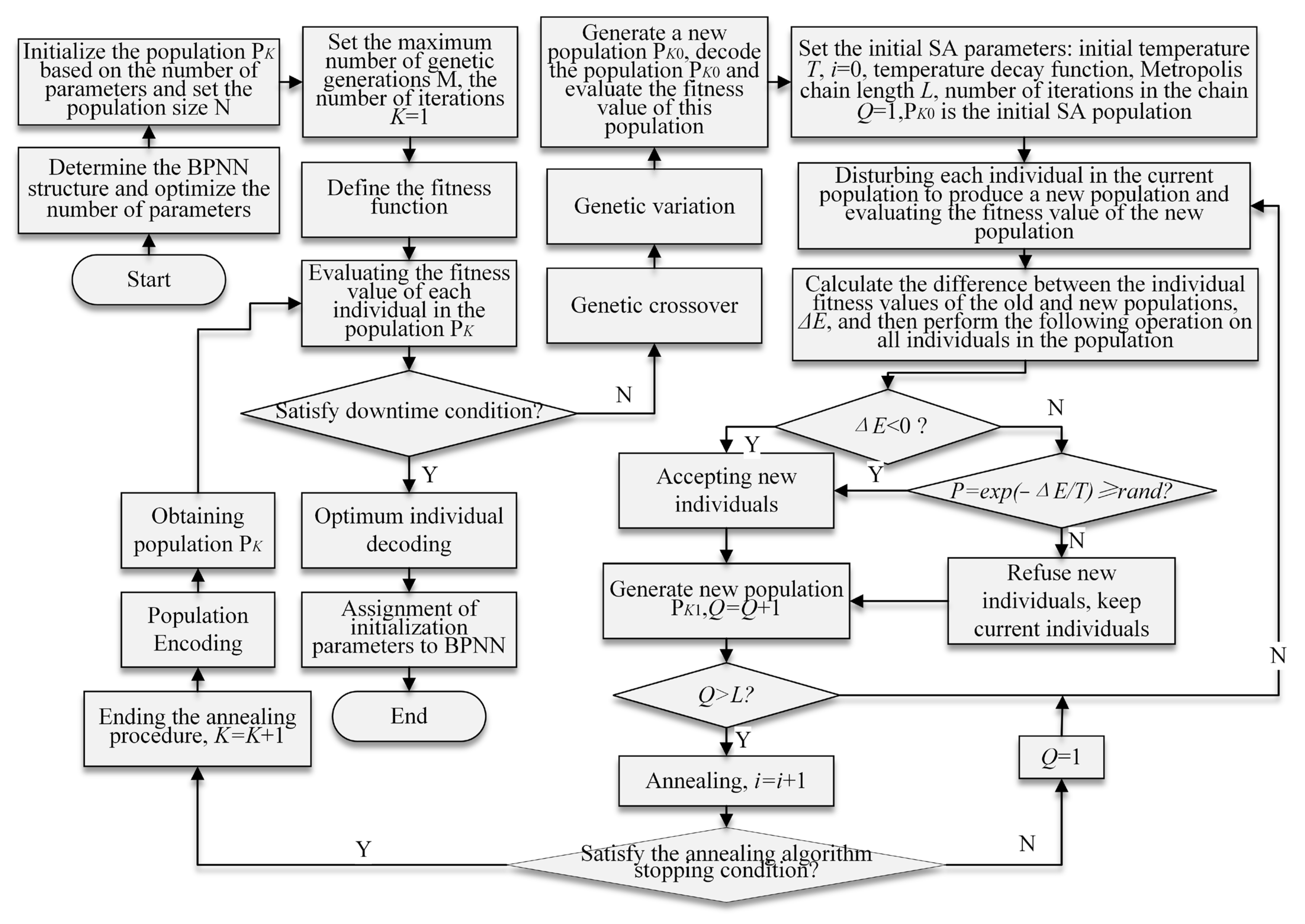
GA Initialization: Set the population size N and initialize the population P_K. Set the maximum number of generations M and the genetic iteration number K to 1;

(2)

Defining the fitness function;

(3)

Assess the fitness value of the P_K: Verify if the stopping criterion for the GA has been attained. If the criterion has indeed been met, then it yields the most superior solution. If not, proceed with steps (4) to (9) accordingly;

(4)

P_K performs genetic crossover and mutation to generate a fresh population, P_K0, and subsequently assesses the fitness value of P_K0.

(5)

Initializing SA parameters: Set the initial solution P_K0 of the population as the initial solution of SA, set i = 0, set the initial temperature T = T_i (sufficiently high), determine the length of the Metropolis chain L at each state T, and set the iteration count in the chain Q = 1.

(6)

At the present temperature T, and for Q = 1, 2, 3, …L, iterate through steps (7) to (9) repeatedly.

(7)

For every member of the current population, induce a random perturbation to generate a fresh population, and subsequently evaluate the fitness of this new population.

(8)

For each member of the current population, determine the disparity in fitness between the fresh population and the current population, represented by $∆E$. Determine whether $P=\exp \left(-\frac{∆E}{T}\right)\ge \mathit{rand}$, and if so, accept the new solution as well; if not, reject the new solution.

(9)

Increment Q by 1. Verify if Q > L. If this condition is satisfied, then increment i by 1, and reduce the temperature using the temperature annealing function such that T = T_i+1, where T < T_i+1. Subsequently, verify if the annealing stopping criteria have been met. If so, then increment K by 1, produce the optimal group solution P_K, and return to step (3). If the annealing stopping criteria have not been met, then set Q to 1, and return to step (7). If Q > L is not met, then return to step (7). The annealing stopping criterion is typically established as the stopping temperature.

(10)

Once the genetic operations have been applied to the P_K population to produce the P_K0 population, the P_K0 population is employed as the initial solution for the SA algorithm to create P_K+1. If the new P_K+1 population does not meet the stopping criteria for the GA, then the population formed by the SA algorithm, P_K+1, is adopted as the starting population for the GA to partake in the iterative optimization.

2.1.2. Performance Testing of the GASA Algorithm

The GASA is a random search algorithm, and Rastrigin’s function was chosen to test its optimization performance due to its numerous local optima, which can mislead algorithms. Therefore, it is an ideal choice for testing the performance of algorithms. Figure 3 displays a three-dimensional plot of the function. The mathematical expression for this function is as follows:

$$\mathit{Ras}\left(x\right)=20+x_1^2+x_2^2-10\left(\cos 2\pi x_1+\cos 2\pi x_2\right)$$

(1)

where $x_1\in \left[-5,5\right],x_2\in [-5,5]$

To optimize the function, the GASA algorithm’s parameters can be customized before executing the algorithm. In addition, the PSO, GA, and SA algorithms can also be utilized individually for function optimization. A performance test through experimental analysis can be conducted to compare the performance of each algorithm. Given that these algorithms are all stochastic search algorithms, it is advisable to conduct multiple experiments to avoid significant accidental errors. Therefore, each algorithm can be tested 20 times under identical environmental conditions. The termination condition for each algorithm can be set to exceed 200 iterations or reach the global minimum value during optimization. The outcome of these experiments is presented in

Table 1. The table of optimization results for the test function.

Algorithm	Test Function	Average Result	Variance of Results
PSO	Rastrigin’s function	9.2472 × 10−4	3.1547
GA		7.9003 × 10−3	3.7519
SA		9.1873 × 10−2	7.6823
GASA		5.6935 × 10−4	2.0524

.

After analyzing the test outcomes presented in Table 1, it is apparent that the algorithms did not achieve the set objectives in every one of the 20 optimization runs. Additionally, the number of iterations and optimization results varied for each algorithm. Upon examining the performance metrics of average optimization value, variance of optimization results, and average number of iterations, it is evident that the GASA algorithm exhibits superior function optimization capabilities and global search stability compared to the PSO, GA, and SA algorithms.

Figure 4 illustrates the curve of the best individual’s average fitness function value during the function optimization process. The GASA algorithm reaches the optimal value at the 78th iteration, the PSO reaches the optimal value at the 102nd iteration, and the GA and SA algorithms converge at the 156th and 176th iterations, respectively. However, the fitness function value quality of the latter two algorithms is inferior to that of the former two. Consequently, when compared to the PSO, SA, and GA algorithms, the GASA algorithm demonstrates better performance and efficiency in the complex function parameter optimization process.

2.2. Development of a Gas Content Prediction Model Based on the GASA-BPNN Algorithm

BP theory was originally proposed by Werbos in 1974, and it served as a cornerstone for the development of artificial neural networks [26,28]. In 1986, Rumelhart and McClelland introduced the error backpropagation learning algorithm, which is used for training multilayer neural networks. The neural network trained using the BP algorithm is referred to as the BP neural network (BPNN). The BPNN is a multilayer feedforward neural network that is trained using the error backpropagation algorithm. It comprises an input layer, several hidden layers, and an output layer, with each layer being connected through different weight parameters in a fully connected manner. Research has demonstrated that a single hidden layer BPNN has the ability to arbitrarily approximate any complex nonlinear system, as depicted in Figure 5.

An insufficient number of hidden layer nodes in a BPNN can result in underfitting and low prediction accuracy, while an excessive number of nodes can lead to overfitting. The range of nodes is determined based on empirical Formula (2) and found to be [4,12]. The optimal number of nodes is selected by comparing the average relative prediction error of the model, and the results are presented in

Table 2. Number of hidden layer nodes and the average relative error table.

W	4	5	6	7	8	9	10	11	12
Relative Error/%	27.9	30.84	21.29	19.73	24.18	19.62	16.35	21.87	15.22

. The table demonstrates that the error is minimized when the number of nodes is W = 12, indicating that 12 nodes are optimal. Research has revealed that a three-layer BPNN can effectively approximate any complex nonlinear system; therefore, the GASA-BPNN prediction model is structured as a 6-12-1 BPNN.

$$W=\sqrt{c+q}+B$$

(2)

The variables in the equation are defined as follows: W denotes the count of nodes in the hidden layer, c represents the number of nodes in the input layer, q signifies the number of nodes in the output layer, and B is an integer ranging from 1 to 10.

Figure 6 depicts the process of applying the model, while Figure 7 shows the GASA-BPNN gas content prediction model. The application steps are described below in detail [16]:

(1)

To apply the prediction model, the data are first normalized to the range of [0, 1]. Subsequently, the dataset is stratified and sampled into 10 mutually exclusive subsets. Each time, one subset is chosen as the test set, while the remaining subsets are used as training sets for 10 rounds of training and testing. Figure 8 illustrates the schematic diagram of the sample division process.

(2)

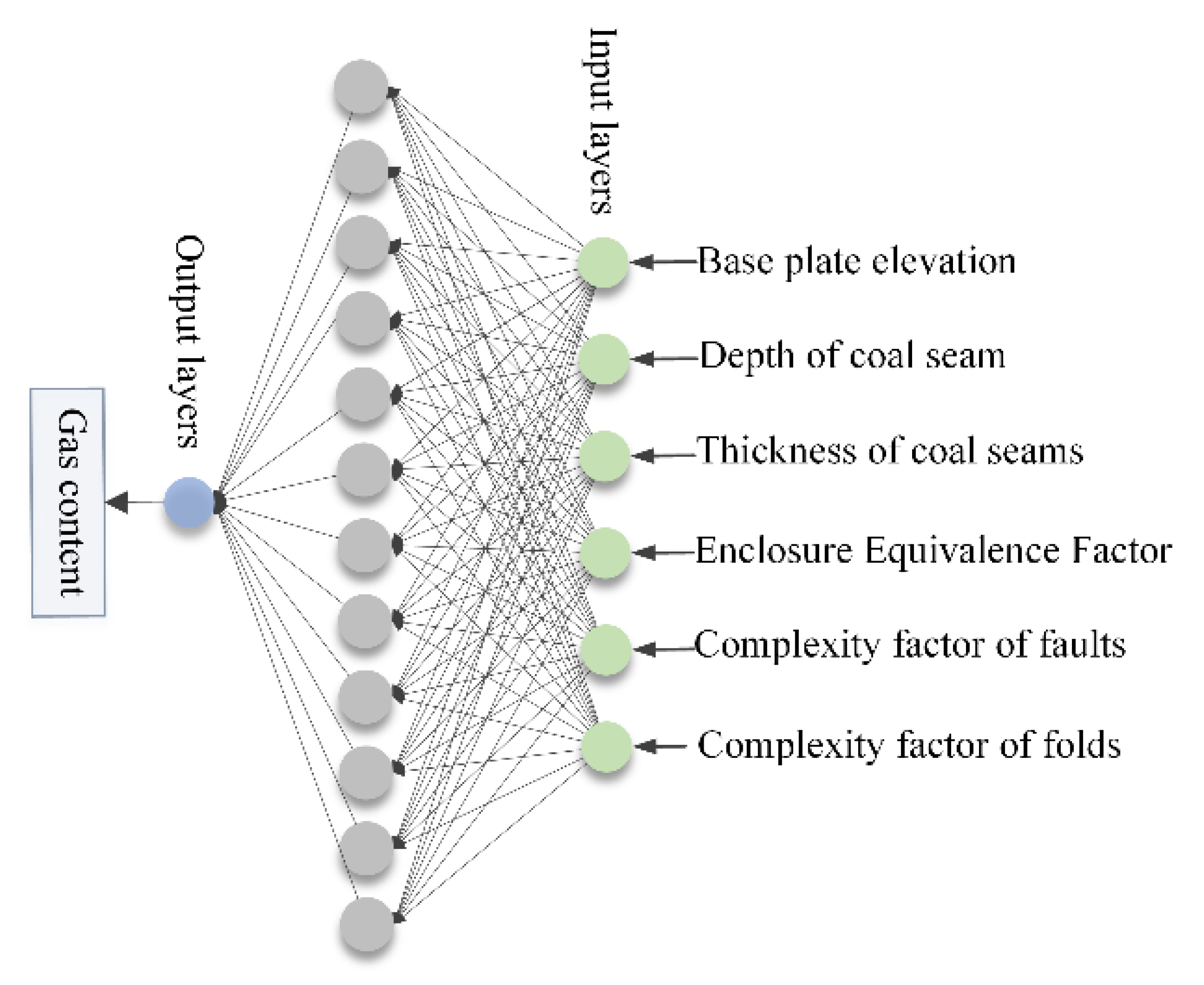
The initialization of the GA population involves encoding the 97 parameters using floating point number encoding rules. Each individual in the population represents a unique set of weights and thresholds. The initial population, P_K, consists of 50 individuals who are randomly generated.

(3)

The GA parameters are set as follows: The maximum number of genetic iterations is set to 800, K is initialized to 1, and the GA stops when the maximum number of iterations is reached. The crossover probability is set to 0.7, and the mutation probability is set to 0.005.

(4)

The fitness function is defined based on the MSE of the prediction, whereby a smaller MSE value yields a higher fitness value for the individual.

(5)

The initial population P_K was subjected to fitness evaluation, and the individuals were ranked based on their respective fitness values.

(6)

Stopping criteria for GASA: Check if the maximum number of genetic iterations has been reached. If so, then terminate the process and proceed to steps (7)–(11). Otherwise, increment K by 1 and proceed to step (12).

(7)

BPNN Initialization: The solution obtained from step (6) is assigned to the BPNN. The maximum number of training iterations is set to H = 800, and the iteration counter is initialized to S = 0.

(8)

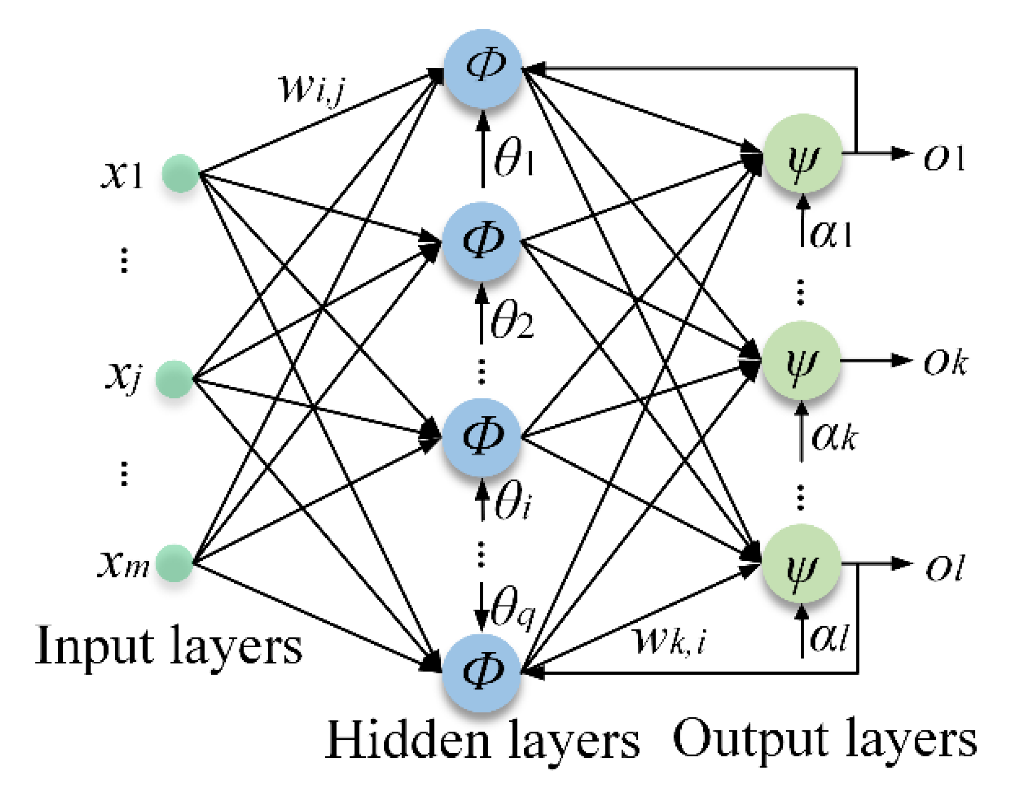
The input dataset is processed by propagating the data forward through the layers of the BPNN. The input for the fth neuron in the hidden layer is computed using Equation (3), and the input for the jth output node is computed using Equation (4).

$${\gamma }_f={\sum }_{v=1}^5{v}_{vf}{x}_v$$

(3)

where ${\gamma }_f$ represents the input of the hidden layer neuron f and $v_{vf}$ represents the weight of the connection between the input layer neuron v and the hidden layer neuron f.

$${\beta }_j={\sum }_{f=1}^{12}{w}_{\mathit{fj}}{b}_f$$

(4)

where ${\beta }_j$ is the input of output node j; $w_{\mathit{fj}}$ is the weight of the connection between intermediate layer node f and output layer node j; and $b_f$ is the output of intermediate layer node f.

(9)

The BPNN weights and thresholds are updated by backpropagating the MSE to each node, and the parameters are adjusted using the error-adaptive learning rate gradient descent method described in Equation (5). If the error approaches the target value with less fluctuation, then the model training direction is correct, and the learning rate can be increased. However, if the error increases beyond the allowed range, then the model training direction is incorrect, and the learning rate should be reduced.

$$\mu \left(S+1\right)=\left\{\begin{array}{c}{S}_{\mathit{in}}\mu \left(S\right),E\left(S+1\right)<E\left(S\right)\\ S_{\mathit{de}}\mu \left(S\right),E\left(S+1\right)>E\left(S\right)\end{array}\right.$$

(5)

where $\mu \left(S+1\right)$ is the learning rate when the number of iterations is S+1; $\mu \left(S\right)$ is the learning rate when the number of iterations is S; $S_{\mathit{in}}$ is the incremental coefficient; $S_{\mathit{de}}$ is the decremental coefficient; $E\left(S+1\right)$ is the error when the number of iterations is S + 1; and $E\left(S\right)$ is the error when the number of iterations is S.

(10)

BPNN stopping criterion: Verify whether the termination criterion has been met, where the minimum error is defined as the stopping condition. If the criterion is satisfied, then the network completes its learning phase, and the model is established, advancing to step (11). Otherwise, examine if H is equal to S. If true, then return to step (7). Otherwise, increase S by one and go back to step (8).

(11)

The performance evaluation of the model involves testing the model on the test set. The evaluation metrics used to assess the model’s performance are the MSE, iteration number, and relative prediction error.

(12)

The selection process in the GA involves the use of the roulette selection method, which serves to screen individuals based on their fitness values. Specifically, for an individual x_u with a fitness value of f_u, the probability of x_u being selected is given by $p_u=f_u/{\sum }_{j=1}^N{f}_u$.

(13)

The process of GA crossover involves randomly selecting two individuals, $x_1$ and $x_2$, from the population P_K, and generating new individuals, $x_1^{\prime }$ and $x_2^{\prime }$, through the arithmetic crossover operation outlined in Equation (6).

$$\left\{\begin{array}{c}{\mathit{x}}_1^{\prime }={\lambda }_1{\mathit{x}}_1+{\lambda }_2{\mathit{x}}_2\\ {\mathit{x}}_2^{\prime }={\lambda }_1{\mathit{x}}_2+{\lambda }_2{\mathit{x}}_1\end{array}\right.$$

(6)

where ${\lambda }_1+{\lambda }_2=1$,${ \lambda }_1>0$, and ${\lambda }_2>0$.

(14)

For the GA variation, an individual genotype X = x₁x₂…x_b…x_s is randomly selected, and the genetic operation is performed at the mutation point x_b using Equation (7).

$$x_b^{\prime }=\left\{\begin{array}{c}{x}_b+∆\left(K,\mathit{UB}-x_b\right),r\le 0.5\\ x_b-∆\left(K,x_b-\mathit{LB}\right),r>0.5\end{array}\right.$$

(7)

Here, UB and LB denote the upper and lower boundary values of the variable x_b, respectively. r represents a random number, and K denotes the evolutionary algebra. Furthermore, $∆\left(t,y\right)$ is a function defined as follows:

$$∆\left(t,y\right)=y\left[1-r^{{\left(1-\frac{K}{M}\right)}^q}\right]$$

The nonconsistency control parameter q (set to q = 0.8) is used in the above equation.

(15)

Evaluate the fitness of P_K0: Calculate the fitness value of P_K0 and designate it as the initial population of the annealing algorithm.

(15)

SA parameter initialization: All genetically operated individuals undergo annealing. The initial temperature T is set to 100 °C, the cooling factor is set to 0.98, and the stopping criterion is set such that Q = 1 and the Markov chain length is L = 60.

(17)

A novel solution is produced by perturbing each member of the population, computing the disparity between the fitness values of each member in the old and new populations, and determining whether to adopt the new solution based on the Metropolis sampling criterion.

(18)

Increment Q by 1 and check if it is in the current Markov chain. If it is in the chain, then proceed to step (17). If it is not in the chain, then decrease the temperature and check if the stopping condition for the SA is met. If the stopping condition is met, then the SA algorithm ends and proceeds to step (4). Otherwise, set Q = 1 and proceed to step (17).

2.3. Establishment of a Gas Content Prediction Model Based on the GASA-SVM Algorithm

The theory of SVM encompasses optimal classification hyperplanes, kernel functions, and margin theory. The SVM offers several advantages, such as suitability for handling small sample sizes, robust generalization ability, and simple structure. In a wide range of domains, including medicine, electricity, and economics, SVMs have found practical applications for pattern recognition and regression problems [29,30].

The fundamental tenet of SVM is to identify the optimal classification hyperplane in the sample space that can segregate various classes of samples while minimizing the empirical and structural risks associated with the classifier. To illustrate the principle of SVM for linear classification in two dimensions, consider the example shown in Figure 9. The orange circles denote one class of samples, while the blue circles correspond to another class. The classification line for these samples is represented by H, whereas H₁ and H₂ are two parallel lines that pass through the points of the two classes that are closest to the classification line. The distance between H₁ and H₂ is known as the classification margin. To enhance the model’s generalization ability, it is crucial to maximize the classification margin, indicating that the greater the margin, the more robust the model’s generalization ability to unobserved examples and the higher the accuracy of the model’s prediction.

Sample $D=\left\{\left({\mathit{x}}_1,y_1\right),\right.\left.\left({\mathit{x}}_2,y_2\right),\dots ,({\mathit{x}}_m,y_m)\right\},y_i\in \mathbb{R}$, conventional regression models evaluate prediction error by directly computing the difference between the predicted value of the model and the actual value y. A fitting error of zero is achieved only when the predicted value matches y precisely. However, support vector regression uses a different method to calculate errors. SVR permits a maximum error of $ϵ$ between the predicted value and the measured value, assuming that the deviation between the predicted value and the measured value is zero. Figure 10 illustrates this concept, with the red line representing the true value and the black circle representing the predicted value. A sample is accurately predicted if the predicted values of the training set fall within the interval band created by the central line of f(x) with a width of 2$ϵ$, resulting in a prediction error of zero.

The selection of the kernel width parameter and regularization factor has a profound impact on the predictive performance of SVM. However, traditional grid search algorithms have limitations, such as undefined value ranges and large computational costs. To overcome these challenges, a GASA algorithm is proposed to initialize the core parameters of SVM. The optimized parameters are then assigned to SVM, and the GASA-SVM gas content prediction model is established by training the SVR machine with the original data. Since the process of initializing SVM and ELM parameters using the GASA algorithm is similar to the process of initializing BPNN parameters, in the following text, only the key steps of the initialization process for SVM and KELM are retained.

The process of constructing the GASA-SVM prediction model is depicted in Figure 11. The steps involved in building the model are as follows:

(1)

The 10-fold cross-validation method is used to split the data into test and training sets;

(2)

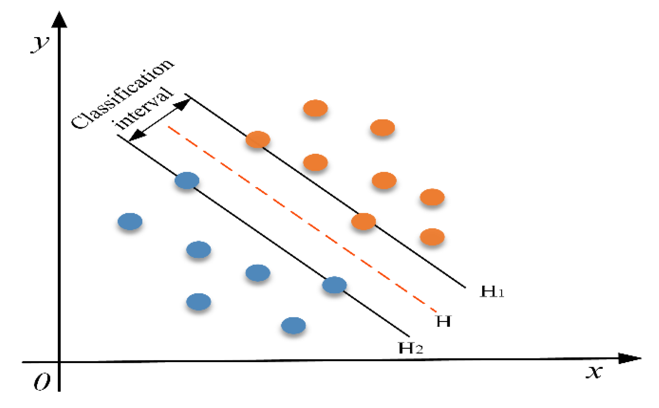
GA initialization: The parameters σ and c of the kernel function are encoded using the floating-point number encoding rule. A population of 50 individuals is randomly initialized, and the population size and GA parameters such as maximum generation and crossover probability are set;

(3)

Fitness evaluation function: The MSE between the predicted gas content and the actual output is minimized as the fitness evaluation function. The randomly initialized individuals from step (2) are evaluated. The genetic stopping condition is checked. If met, then the optimal individual is output, decoded, and assigned to SVM. GASA completes the optimized SVM, which is then trained again using the sample data to establish the model. If the genetic stopping condition is not met, then genetic crossover and genetic mutation are performed. The resulting individuals are used as the initial generation population of the SA algorithm;

(4)

SA algorithm initialization: Individuals in the population that did not meet the genetic stopping condition in step (3) are used as the initial individuals in the SA algorithm. Each individual undergoes simulated annealing. The initial parameters of SA, such as the initial temperature, temperature decay function, and Metropolis chain length, are set. Essentially, an SA algorithm is concatenated under each individual in the GA population;

(5)

Interference population: Each individual in the population generates a new population using the fitness evaluation function in step (3). The fitness function value is evaluated, and the difference in fitness function value between new and old populations is calculated. Finally, the Metropolis sampling criterion is used to determine whether the old solution should be replaced by the new solution;

(6)

Check if the SA stopping condition is met. If it is met, then end the annealing and use this population as the next generation population in the GA in step (3). If it is not met, then return to step (5).

2.4. Development of a Gas Content Prediction Model Based on the GASA-KELM Algorithm

Multilayer feedforward neural networks (FFNNs) have been widely used in linear and nonlinear system identification due to their excellent global approximation performance [31]. However, most traditional FFNN learning algorithms are based on the gradient descent method to modify all the weights and thresholds of the entire network. This has the disadvantages of requiring a large number of iterations, which makes it difficult to select an appropriate learning rate. To overcome the shortcomings of traditional FFNN algorithms, Huang Guangbin proposed a new algorithm called ELM for solving single-hidden-layer feedforward neural networks [32]. Compared with traditional algorithms, ELM randomly initializes the connection weights and thresholds of FFNN and does not participate in learning and correction. The unique optimal solution can be obtained by adjusting the number of hidden layer nodes.

The proposed model for predicting gas content in coal seams based on the improved ELM introduces the radial basis function kernel due to the nonlinear nature of the gas content prediction system. The initial kernel parameters, which include the bandwidth of the Gaussian kernel and regularization factor of KELM, have a significant impact on the model’s predictive performance. The issue of randomly assigned kernel parameters leading to a non-full rank output matrix can weaken the model’s ability to generalize to new data. To address these issues, a hybrid heuristic algorithm is constructed to optimize the kernel parameter $\sigma$ and regularization factor C of ELM.

Figure 11 illustrates the process of constructing the GASA-KELM model for predicting gas content in coal seams. The model building process involves the following steps:

(1)

Normalize the dataset and split it into training and testing sets using 10-fold cross-validation.

(2)

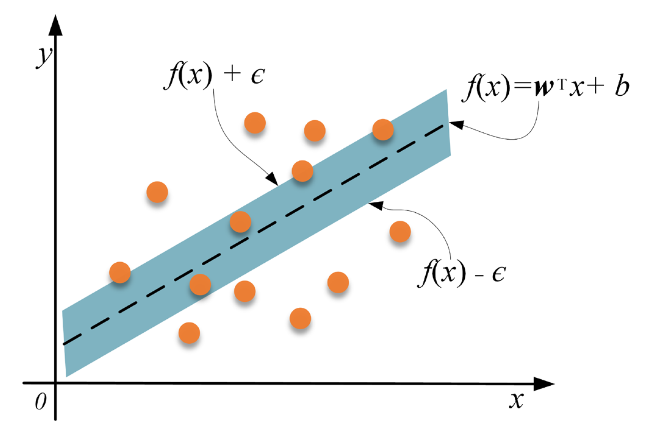
Initialize the GA by encoding the kernel function parameters $\sigma$ and penalty factor c for the KELM, randomly initializing the population, and setting the population size and GA parameters.

(3)

Define the fitness evaluation function as the MSE between the predicted and actual values of the model, and evaluate the randomly initialized individuals in the population from step (2). Determine if the genetic stopping condition is met. If so, then output the optimal individual, decode it, and assign it to KELM. Complete the model establishment by training the sample data again. The training process and model performance evaluation are discussed in the following section. If the genetic stopping condition is not met, then perform genetic operations, and use the resulting individuals as the initial population for SA.

(4)

Initialize the SA algorithm by using the population individuals from step (3) that did not meet the genetic stopping condition as the initial population for the SA algorithm. Each individual undergoes simulated annealing. Set the initial parameters for SA, such as the initial temperature, temperature decay function, and Metropolis chain length, which correspond to an SA algorithm linked to each population individual in the GA.

(5)

Update the population using the neighborhood function to generate a new population. Evaluate the fitness function value using the evaluation function from step (3), calculate the difference in fitness values between the new and old populations, and determine whether to replace the old solution based on the Metropolis criterion.

(6)

Determine whether the annealing stopping condition is met. If it is met, then complete the annealing operation and use this population as the next generation population in the GA in step (3). If it is not met, then return to step (5).

3. Field Application of Gas Content Prediction Models

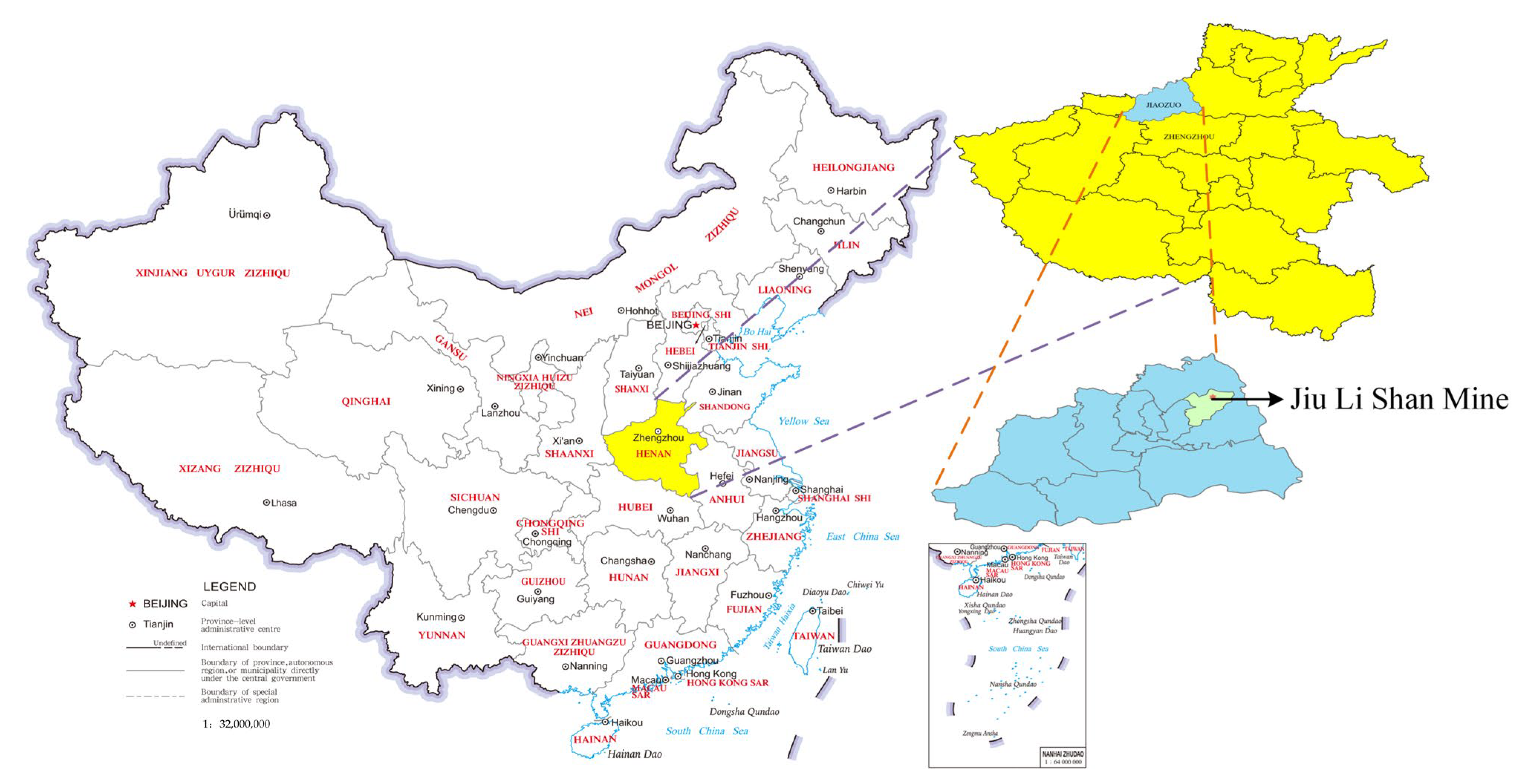
3.1. Overview of the Jiulishan Mine in Jiaozuo

The Jiulishan Mine is situated in the heart of the Jiaozuo mining area, approximately 18 km from Jiaozuo city. The mine spans an area of approximately 18.7 km², with a north-south width of approximately 3.4 km and an east-west length of approximately 5.5 km. Its construction began in July 1970, and it commenced simple production in April 1983. The mine was designed to have a production capacity of 900,000 tons per annum, with a rated production capacity of 1 million tons per year. The vertical shaft mining method and combined development of upper and lower levels are employed in the mine. The coal seam that is mined is the Shanxi Formation II-1 coal seam, which has a simple structure and stable occurrence and is a medium-gray, low-sulfur, high-quality anthracite with a thickness ranging from 0.92 m to 8.13 m and an average thickness of 5.15 m. Its recoverable reserves index is 97.5%. The Jiulishan Mine is known for its coal and gas outburst, and its primary regional gas control measures include the combination of bottom rock roadway cross-layer predrainage of coal seam gas in the premining area and the drilling of in-seam boreholes to predrain coal seam gas in the mining area.

The Jiulishan Mine employs a central parallel and diagonal mixed ventilation system, utilizing a mechanical extraction method. The main and auxiliary shafts, in addition to the West Ventilation Shaft, are designated as intake airways, while the East and South Ventilation Shafts function as return airways. At present, the mine’s total intake air volume stands at 13,500 m³/min, while the total exhaust air volume is 13,820 m³/min. The absolute gas emission rate of the mine is 43.99 m³/min, with a corresponding relative gas emission rate of 33.41 m³/t. The mine’s location can be seen in Figure 12.

3.2. Establishment of the Parameter System for the Gas Content Prediction Model

3.2.1. Establishing a Dataset for Gas Content Prediction

Based on an analysis of the gas geological conditions and distribution patterns in the 15th mining area of the Jiulishan Coal Mine in Henan Province, China, we have identified eight factors that can quantitatively affect gas content (X₀, m³·t⁻¹): coal seam depth (X₁, m), coal seam thickness (X₂, m), dip angle coefficient (X₃), overlying rock thickness (X₄, m), surrounding rock equivalent coefficient (X₅), fault complexity coefficient (X₆), fold complexity coefficient (X₇), and floor elevation (X₈, m) [33,34]. In the 15 mining areas, 290 sets of data on gas content and influencing factors were selected as the experimental dataset. The training sample data for the model are shown in

Table 3. Part of the model training sample data.

Sample Number	X0/(m3·t−1)	X1/(m)	X2/(m)	X3	X4/(m)	X5	X6	X7	X8/(m)
1	17.01	407.12	6.44	0.0198	254.09	0.4185	0.0008	0.0005	−324.81
2	25.32	350.41	6.08	0.0191	209.54	0.9000	0.1416	0.1812	−265.47
3	25.63	327.86	5.74	0.0354	191.74	0.4508	0.3062	0.0001	−243.64
4	15.27	438.26	4.84	0.0213	241.67	0.4000	0.0016	0.0001	−353.7
5	18.99	363.62	5.79	0.0440	219.25	0.5663	0.1003	0.0004	−279.48
6	12.53	400.92	3.61	0.0193	256.23	0.7740	0.0264	0.0048	−315.06
7	22.03	524.6	5.35	0.0122	267.32	0.5109	0.3255	0.0025	−437.3
8	21.46	517.3	4.36	0.0171	114.52	0.3855	0.0853	0.0115	−430
9	24.46	437.4	4.81	0.0224	121.89	0.2370	0.1189	0.0137	−350.7
10	24.03	444	7.07	0.0165	188.67	0.6074	0.0352	0.0084	−359.82
11	31.01	305.42	5.39	0.0403	207.99	0.3394	0.1738	0.0002	−217.27
12	19.17	326.7	5.43	0.0546	241.06	0.5873	0.0032	0.0117	−242.16
13	27.63	530	10.59	0.0412	334.41	0.4105	0.0421	0.0004	−440.9
14	20.41	501.7	5.34	0.0159	128.22	0.3534	0.0266	0.0010	−414.5
15	9.67	284	5.62	0.0166	144.48	0.3299	0.0338	0.0012	−195.1
16	18.86	438	5.07	0.0154	95.09	0.4837	0.0984	0.0029	−350.4
17	16.71	400.92	3.6l	0.0278	256.23	0.7740	0.0264	0.0048	−317.1
18	12.74	400.92	3.61	0.0315	256.23	0.7740	0.0009	0.0001	−308.68
19	27.86	309.48	5.80	0.0302	174.28	0.3158	0.1480	0.0008	−220.93
20	13.38	474.73	2.66	0.0222	306.27	0.3718	0.0015	0.0005	−383.68

.

3.2.2. Primary Controlling Factors of Gas Content Based on Grey Correlation Analysis

The prediction of gas content is a challenging nonlinear prediction problem that is affected by various factors. Grey system theory is a suitable method for such problems with limited data, and grey correlation analysis can determine the extent to which each reference sequence affects the parent sequence. The quantitative ordering of correlations provides a clear comprehension of the relationship between various influencing factors and helps identify the principal controlling factors of gas content.

The GRA method is used to screen the main controlling factors for the model’s input. The steps of the grey relational calculation are as follows [35]:

(1)

Setting reference sequence and comparison sequence: Reference sequence: Gas content (X₀), Comparison sequence: Eight influencing factors of coal seam gas content.

(2)

Data preprocessing and normalization: According to Formula (8), the data will be normalized.

$$x_l^{\prime }\left(h\right)=\frac{x_l\left(h\right)-x_{\mathit{min}}}{x_{\mathit{max}}-x_{\mathit{min}}}$$

(8)

where $x_l\left(h\right)$ is the value of the l-th evaluation index of the sample with the number h; h represents the sample number, h = 1, 2, …, n; l represents the evaluation index, l = 1, 2, …, m; and x_max and x_min are the maximum and minimum values of the evaluation index, respectively.

(3)

To calculate the correlation coefficient: The calculation of correlation coefficient is obtained according to Formula (9).

$${\xi }_e\left(k\right)=\frac{\underset{e}{\mathit{min}} \underset{k}{\mathit{min}}\left|x_0\left(k\right)-\right.\left.x_e\left(k\right)\right|+\rho \underset{e}{\mathit{max}} \underset{k}{\mathit{max}}\left|\left.x_0\left(k\right)-x_e\left(k\right)\right|\right.}{\left|x_0\left(k\right)-\right.\left.x_e\left(k\right)\right|+\rho \underset{e}{\mathit{max}} \underset{k}{\mathit{max}}\left|\left.x_0\left(k\right)-x_e\left(k\right)\right|\right.}$$

(9)

The symbol ${\xi }_e\left(k\right)$ denotes the correlation coefficient of the comparison sequence $x_e$ with respect to the reference sequence $x_0$ on index k, where k ranges from 1 to n. The parameter ρ, which takes a value between 0 and 1, is the resolution coefficient.

(4)

To compute the correlation degree: Calculate the correlation degree using Formula (10).

$$r_e=\frac{1}{n}{\sum }_{k=1}^n{w_k\xi }_e\left(k\right)$$

(10)

where n is the number of samples, r_e is the correlation degree of the comparison sequence x_e with the reference sequence x₀, and $w_k$ is the weight of the indicator.

(5)

Ranking of correlation and determination of input parameters

Table 4. The results of grey correlation analysis.

Factors Influencing	X1	X2	X3	X4	X5	X6	X7	X8
$r_e$	0.6698	0.5623	0.2908	0.3176	0.5024	0.6117	0.5102	0.5785

presents the results of the correlation analysis, revealing that the correlation coefficients of the influencing factors X₃ and X₄ fall below 0.5, indicating a low correlation. Consequently, these factors are eliminated. This brings the number of input layer nodes to 6, as the data dimension in Table 3 is reduced from 8 to 6. The six highly correlated gas content influencing factors are the only inputs for the model, whereas the other two factors are no longer involved in the modeling process.

3.3. Parameter Optimization and Testing of the Model

The parameter initialization process involves utilizing the fitness function of the GASA algorithm, which is the MSE between the predicted and actual values, to optimize the initial parameters of the three gas content prediction models. To circumvent the potential issue of stochastic errors that may arise in random search algorithms, the GASA was employed to optimize the parameters of each model for 100 iterations. Figure 13 depicts the average evaluation function values during the parameter optimization process. As observed in the figure, the target requirement was not met within 800 iterations while optimizing BPNN parameters using GASA. Hence, the threshold and weight corresponding to the minimum fitness value were selected as the optimal initial parameters and assigned to the BPNN model to complete the parameter initialization process.

As the SVM and KELM models underwent initial optimization of kernel parameters and penalty factors, optimal initial parameters were discovered by the two models in the 673rd and 487th iterations, respectively. Once these parameters were decoded and assigned values, the initialization process was complete. The results depicted in Figure 13 reveal that the optimization speed and quality of the SVM and KELM parameters with GASA were markedly superior to those of the BPNN, which has a larger number of parameters to optimize.

After initializing each model with optimal initial parameter values, we trained the final models separately using the data collected in Table 3. To evaluate the predictive performance of the GASA-BPNN, GASA-SVM, and GASA-KELM models for gas content prediction, we performed 10-fold cross-validation ten times under identical conditions. In each iteration, the training set and test set were input into the model for 100 iterations of training and prediction. The prediction results for the ten test sets in the 10-fold cross-validation are presented in

Table 5. Ten-fold cross-validation of the prediction results.

——	A1	A2	A3	A4	A5	A6	A7	A8	A9	A10	Average/%	Variance
BPNN	19.46	12.59	16.6	7.53	15.32	17.9	17.82	12.06	20.89	17.21	15.738	3.99
SVM	13.81	15.3	8.74	15.11	18.29	13.76	10.03	15.58	14.71	13.15	13.848	2.76
KELM	12.46	7.92	10.07	8.14	9.24	11.44	13.78	9.16	8.35	8.09	9.865	2.05

. As observed from Table 5, the variance of the average relative error and the total average relative error for the coalbed methane prediction by the GASA-SVM and GASA-KELM models in each of the ten test sets is lower than that of the GASA-BPNN model. This suggests that the accuracy and stability of the SVM and KELM models for methane content prediction are superior to those of the GASA-BPNN model.

In the final stage of the study, 12 sets of samples were designated as validation sets, and the three models were utilized to predict the gas content of these samples. The predictive performance of the 12 validation samples, which were included in the test set of all 10 simulated tests, was analyzed, and the prediction outcomes of the three models were compared. The results of the validation sample predictions for the three models are presented in Figure 14.

Based on the graph, it can be observed that the predicted values of GASA-KELM are in closer proximity to the actual values than those of GASA-BPNN and GASA-SVM. Moreover, the GASA-KELM model displays smaller average relative errors and exhibits less fluctuation in both average relative and absolute errors. Furthermore, the accuracy and stability of the GASA-SVM model surpass those of the GASA-BPNN model. These findings suggest that the GASA-KELM model possesses the most robust prediction stability and highest prediction accuracy for gas content. The prediction performance of GASA-SVM for gas content is only second to that of GASA-KELM, while the performance of GASA-BPNN for coal seam gas content prediction is relatively subpar in comparison.

3.4. Application of the Model in Engineering and Evaluation of Its Predictive Performance

The developed model was successfully applied for on-site prediction of gas content in the 15th mining area of the Jiulishan Coal Mine in Jiaozuo, Henan. However, it should be noted that the model was developed based on the gas content and related influencing factor data specific to the 15th mining area. This is because different geological units have their own gas geological laws, and the main factors influencing gas content can vary greatly among different mining areas, zones, seams, and mines. Therefore, if the model needs to be applied in a different location, then it is necessary to reanalyze local gas content influencing factors and collect relevant data to retrain the model with new information. Before applying the gas content prediction model on site in the 15th mining area, it is essential to collect gas content influencing factor data from the measurement point. All influencing factors should be carefully recorded, and five sample datasets, as shown in

Table 6. Field application sample data sheet.

Sample Number	X0/(m3·t−1)	X1/(m)	X2/(m)	X3	X4/(m)	X5	X6	X7	X8/(m)
1	24.03	449	4.75	0.0107	199.44	0.3299	0.1264	0.0027	−364
2	17.65	402	5.48	0.0285	183.86	0.3810	0.0298	0.0199	−308.6
3	24.22	305.1	5.39	0.0291	135.74	0.4302	0.0895	0.0615	−218.9
4	19.71	481	6.24	0.0166	118.10	0.5123	0.0135	0.0047	−394.2
5	22.98	387.8	5.55	0.0243	98.24	0.5808	0.0494	0.0012	−295.1

, could be used as a reference.

Upon inputting the data of the five influencing factors of gas content, as listed in Table 6, into the trained model for prediction, the resulting predictions were analyzed for the five samples when they were all in the test set during 10 simulations. The mean predicted results of the three models for the on-site gas content prediction application process are presented in Figure 15.

Based on the results presented in Figure 15, it can be observed that the GASA-KELM model exhibits superior performance in predicting gas content in coal seams, with a maximum relative error of 16.59% and a minimum relative error of 7.93%. The average relative and absolute errors for the prediction are 10.6% and 2.28%, respectively. In comparison, the GASA-SVM model achieves a maximum relative error of 19.89% and a minimum relative error of 9.01%, with average relative and absolute errors of 13.04% and 2.73%, respectively. Meanwhile, the GASA-BPNN model yields a maximum relative error of 20.64% and a minimum relative error of 10.14%, with average relative and absolute errors of 14.31% and 3.18%, respectively. Taking into account both the relative and absolute errors in the prediction, it can be inferred that the GASA-KELM model is more effective in generalizing to new sample data and provides higher accuracy and stability in predicting gas content in new data samples. Thus, it is better suited to meet the goals and requirements for predicting gas content. The GASA-SVM model performs comparably to the GASA-KELM model in terms of accuracy and generalization ability, while the GASA-BPNN model exhibits relatively lower accuracy than the other two models.

4. Conclusions

The main conclusions are as follows:

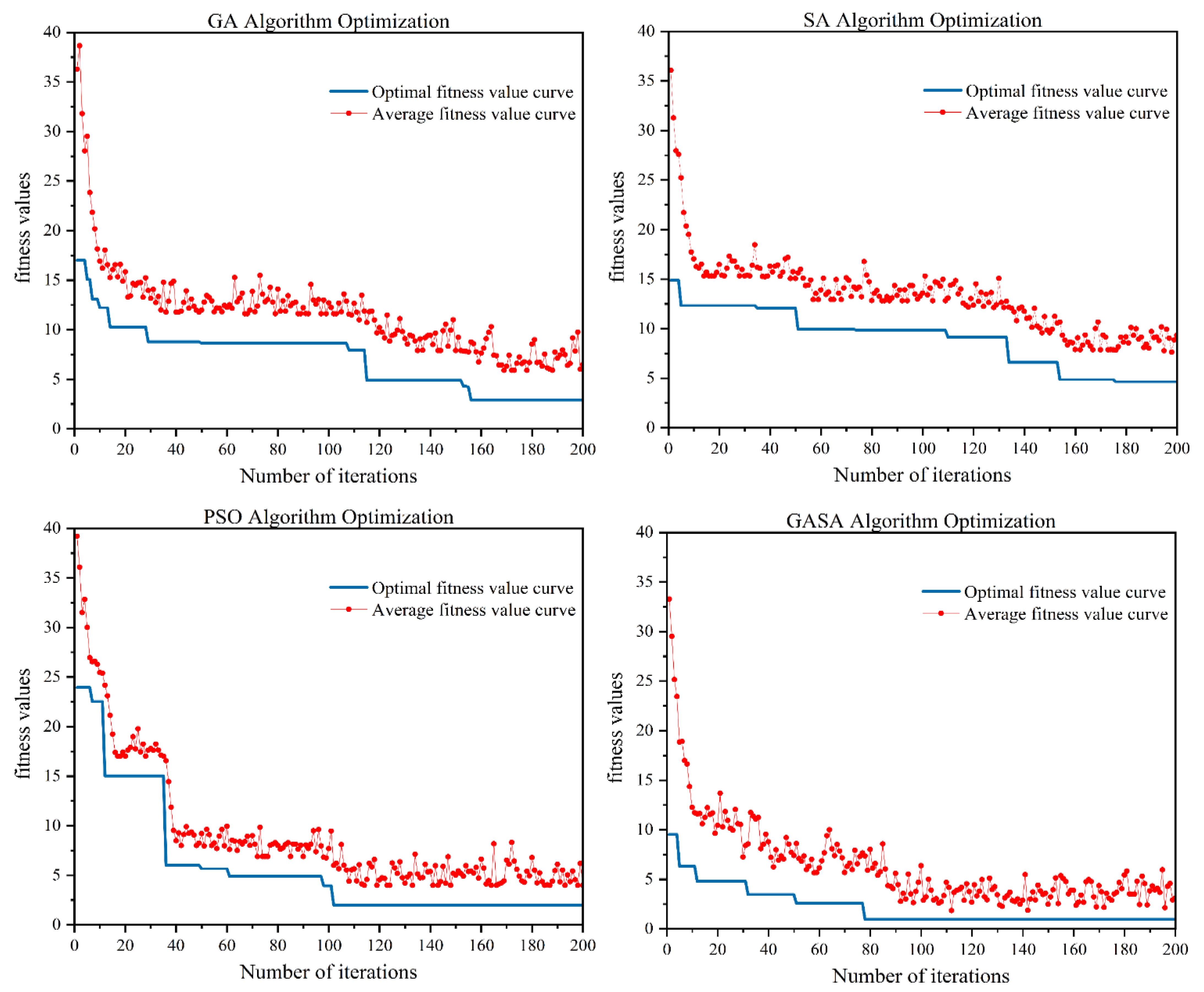
• After conducting verification, Rastrigin’s function was optimized 20 times using the PSO, GA, SA, and GASA algorithms under the same conditions. The algorithms completed the iterative optimization at the 102nd, 156th, 176th, and 78th iterations. The average optimization values of the four algorithms were 9.2472 × 10⁻⁴, 7.9003 × 10⁻³, 9.1873 × 10⁻², and 5.6935 × 10⁻⁴, with respective variances of 3.1547, 3.7519, 7.6823, and 2.0524. After considering the average optimization results over 20 iterations, the variance of the optimization results, and the average number of iterations, the GASA designed in this paper exhibits stronger capabilities in optimizing complex functions and providing stable global search performance compared to the PSO, GA, and SA algorithms. Furthermore, the GASA algorithm demonstrates a more efficient optimization speed and higher optimization accuracy for complex functions compared to single algorithms, effectively avoiding the issue of optimization algorithms being prone to local optima.
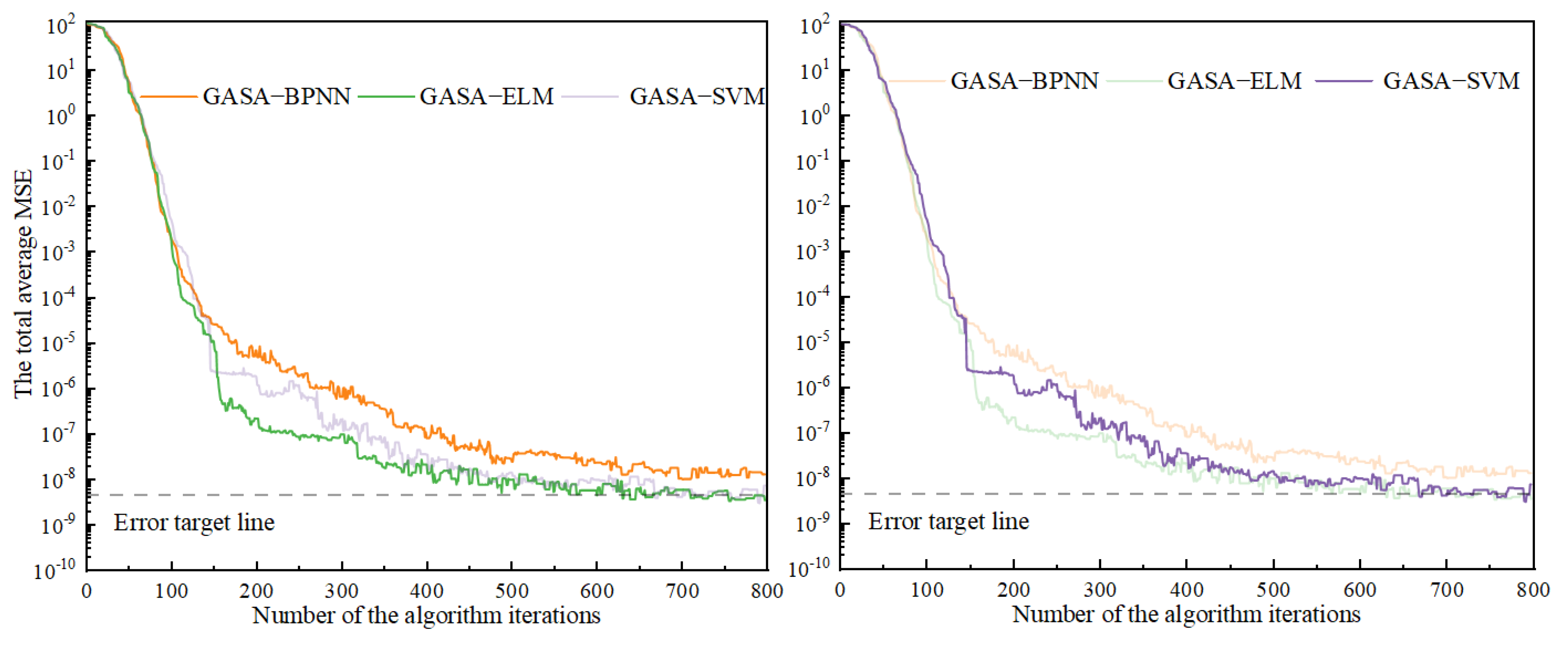
• In the process of constructing the GASA-BPNN prediction model, the GASA failed to meet the target requirements within 800 iterations. Conversely, during the construction of the GASA-SVM and GASA-KELM gas content prediction models, the GASA was able to discover the optimal initial parameters during the 673rd and 487th iterations, respectively. This disparity can be attributed to the fact that the number of parameters to be optimized in BPNN is significantly greater than in SVM and KELM. As a result, the optimization process for the GASA-SVM and GASA-KELM models was much faster and produced higher-quality results than the BPNN model.
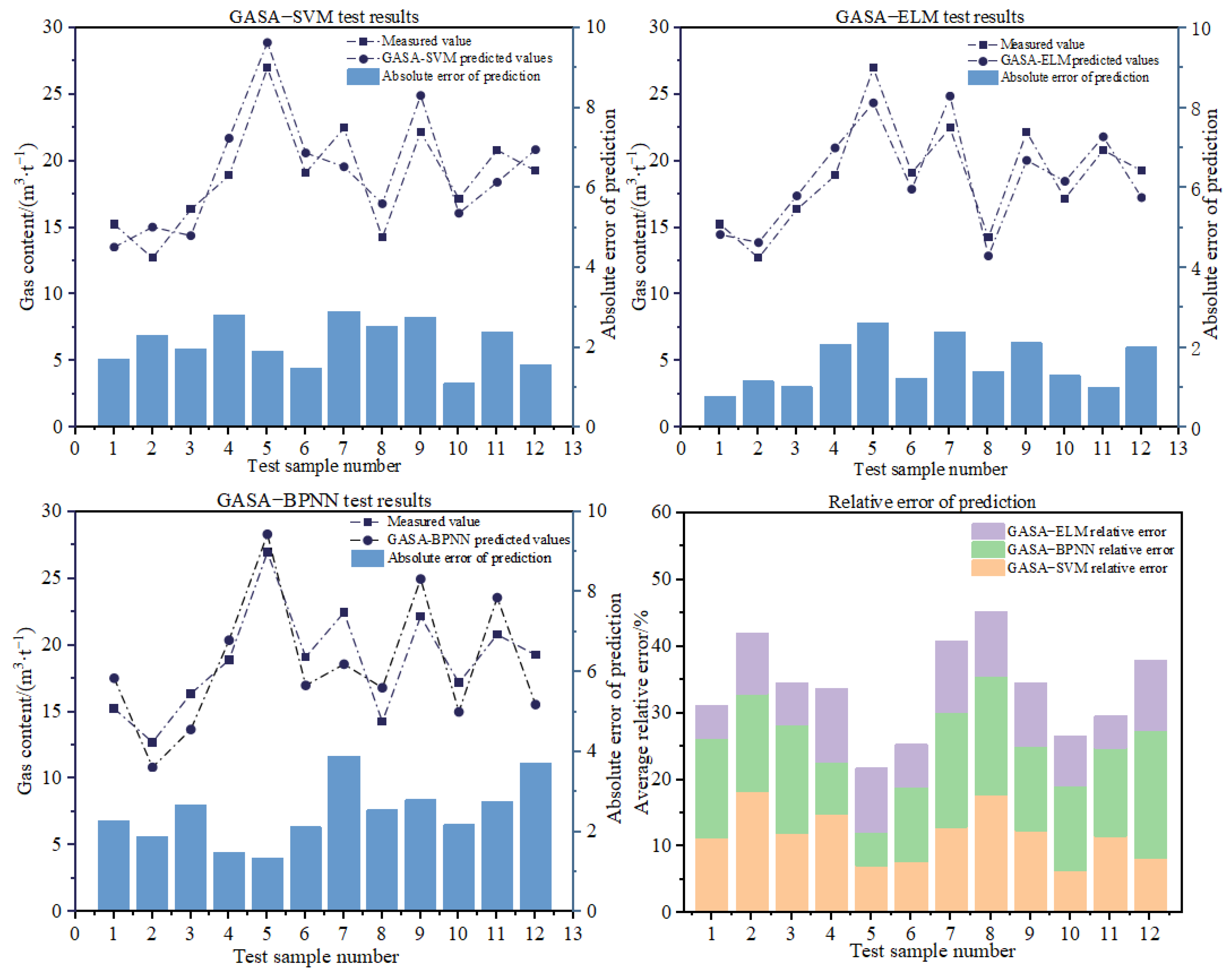
• During 10-fold cross-validation, the GASA-BPNN, GASA-SVM and GASA-KELM models yielded average relative errors of 15.74%, 13.85%, and 9.87%, respectively. The corresponding variances of the 10 cross-validation results were 3.99, 2.76 and 2.05. Notably, in comparison with the GASA-SVM and GASA-BPNN models, the GASA-KELM model displayed superior accuracy and stability in predicting gas content. Subsequently, the GASA-KELM model was tested on twelve additional samples, which further revealed the model’s exceptional performance in terms of prediction accuracy and generalization ability to new sample data.
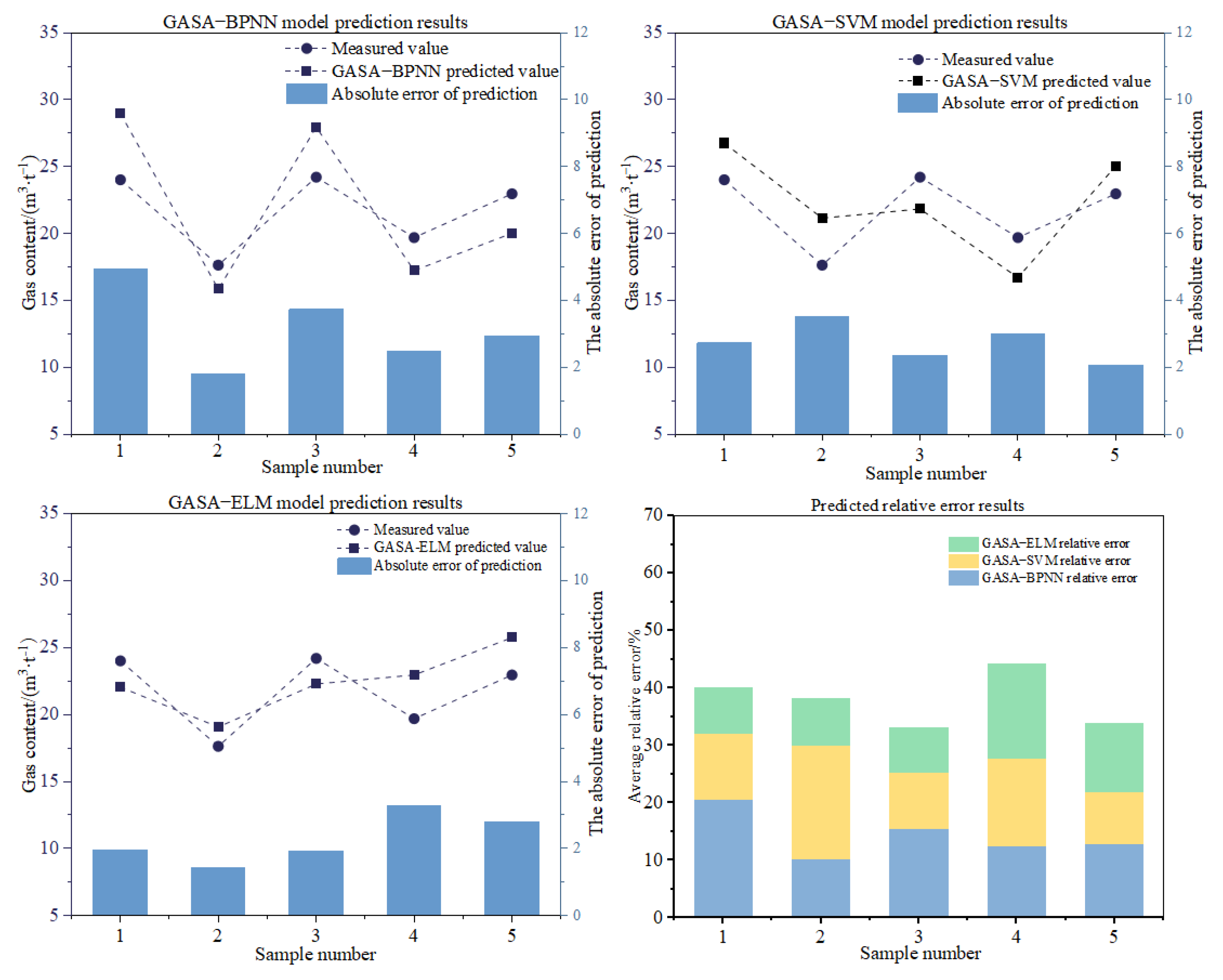
• The developed GASA-KELM model proves to have significant advantages over other ANN models in terms of high accuracy in gas content prediction, stability in prediction, and strong generalization ability when applied to the gas content prediction case of the Jiulishan Mine’s 15-mining area. These advantages are essential for the accurate prediction of gas content and for formulating effective regional gas management strategies.

References

- Wang, S.; Shi, Q.; Wang, S.; Shen, Y.; Sun, Q.; Cai, Y. Resource property and exploitation concepts with green and low-carbon of tar-rich coal as coal-based oil and gas. J. China Coal Soc. 2021, 46, 1365–1377. [Google Scholar] [CrossRef]
- Yuan, L. Scientific conception of precision coal mining. J. China Coal Soc. 2017, 42, 1–7. [Google Scholar] [CrossRef]
- Yuan, L.; Zhang, T.; Zhang, Q.; Jiang, B.; Lv, X.; Li, S.; Fu, Q. Construction of green, low-carbon and multi-energy complementary system for abandoned mines under global carbon neutrality. J. China Coal Soc. 2022, 47, 2131–2139. [Google Scholar] [CrossRef]
- Xu, C.; Wang, K.; Li, X.; Yuan, L.; Zhao, C.; Guo, H. Collaborative gas drainage technology of high and low level roadways in highly-gassy coal seam mining. Fuel 2022, 323, 124325. [Google Scholar] [CrossRef]
- Lin, Y.; Qin, Y.; Wang, X.; Duan, Z.; Ma, D. Geology and emission of mine gas in Binchang mining area with low rank coal and high mine gas. J. China Coal Soc. 2019, 44, 2151–2158. [Google Scholar] [CrossRef]
- Wang, Z.; Wang, L.; Dong, J.; Wang, Q. Simulation on the temperature evolution law of coal containing gas in the freezing coring process. J. China Coal Soc. 2021, 46, 199–210. [Google Scholar] [CrossRef]
- Wang, X.; Zhou, F.; Xia, T.; Xu, M. A multi-objective optimization model to enhance the comprehensive performance of underground gas drainage system. J. Nat. Gas Sci. Eng. 2016, 36, 852–864. [Google Scholar] [CrossRef]
- Wang, S.; Shen, Y.; Sun, Q.; Liu, L.; Shi; Zhu, M.; Zhang, B.; Cui, S. Underground CO2 storage and technical problems in coal mining area under the “dual carbon” target. J. China Coal Soc. 2022, 47, 45–60. [Google Scholar] [CrossRef]
- Fu, X.; Zhang, X.; Wei, C. Review of research on testing, simulation and prediction of coalbed methane content. J. China Univ. Min. Technol. 2021, 50, 13–31. [Google Scholar] [CrossRef]
- Zheng, H.; Zhang, Y.; Liu, J.; Wei, H.; Zhao, J.; Liao, R. A novel model based on wavelet LS-SVM integrated improved PSO algorithm for forecasting of dissolved gas contents in power transformers. Electr. Power Syst. Res. 2018, 155, 196–205. [Google Scholar] [CrossRef]
- Yu, F.; Xu, X. A short-term load forecasting model of natural gas based on optimized genetic algorithm and improved BP neural network. Appl. Energy 2014, 134, 102–113. [Google Scholar] [CrossRef]
- Xin, J.; Chen, J.; Li, C.; Lu, R.; Li, X.; Wang, C.; Zhu, H.; He, R. Deformation characterization of oil and gas pipeline by ACM technique based on SSA-BP neural network model. Measurement 2022, 189, 110654. [Google Scholar] [CrossRef]
- Cao, B.; Yin, Q.; Guo, Y.; Yang, J.; Zhang, L.; Wang, Z.; Tyagi, M.; Sun, T.; Zhou, X. Field data analysis and risk assessment of shallow gas hazards based on neural networks during industrial deep-water drilling. Reliab. Eng. Syst. Saf. 2023, 232, 109079. [Google Scholar] [CrossRef]
- Lin, H.; Gao, F.; Yan, M.; Bai, Y.; Xiao, P.; Xie, X. Study on PSO-BP neural network prediction method of coal seam gas content and its application. China Saf. Sci. J. 2020, 30, 80–87. [Google Scholar] [CrossRef]
- Ma, L.; Lu, W.; Wei, G. Study on prediction method of coal seam gas content based on GASA—BP neural network. J. Saf. Sci. Technol. 2022, 18, 59–65. [Google Scholar]
- Wu, Y.; Gao, R.; Yang, J. Prediction of coal and gas outburst: A method based on the BP neural network optimized by GASA. Process Saf. Environ. Prot. 2020, 133, 64–72. [Google Scholar] [CrossRef]
- Ruilin, Z.; Lowndes, I.S. The application of a coupled artificial neural network and fault tree analysis model to predict coal and gas outbursts. Int. J. Coal Geol. 2010, 84, 141–152. [Google Scholar] [CrossRef]
- Xie, X.; Fu, G.; Xue, Y.; Zhao, Z.; Chen, P.; Lu, B.; Jiang, S. Risk prediction and factors risk analysis based on IFOA-GRNN and apriori algorithms: Application of artificial intelligence in accident prevention. Process Saf. Environ. Prot. 2019, 122, 169–184. [Google Scholar] [CrossRef]
- Meng, Q.; Ma, X.; Zhou, Y. Forecasting of coal seam gas content by using support vector regression based on particle swarm optimization. J. Nat. Gas Sci. Eng. 2014, 21, 71–78. [Google Scholar] [CrossRef]
- Zhang, S.; Wang, B.; Li, X.; Chen, H. Research and Application of Improved Gas Concentration Prediction Model Based on Grey Theory and BP Neural Network in Digital Mine. Procedia CIRP 2016, 56, 471–475. [Google Scholar] [CrossRef]
- Yang, Z.; Zhang, H.; Li, S.; Fan, C. Prediction of Residual Gas Content during Coal Roadway Tunneling Based on Drilling Cuttings Indices and BA-ELM Algorithm. Adv. Civ. Eng. 2020, 2020, 1287306. [Google Scholar] [CrossRef]
- Qiu, L.; Peng, Y.; Song, D. Risk Prediction of Coal and Gas Outburst Based on Abnormal Gas Concentration in Blasting Driving Face. Geofluids 2022, 2022, 3917846. [Google Scholar] [CrossRef]
- Wu, X.; Yang, Z.; Wu, D. Advanced Computational Methods for Mitigating Shock and Vibration Hazards in Deep Mines Gas Outburst Prediction Using SVM Optimized by Grey Relational Analysis and APSO Algorithm. Shock Vib. 2021, 2021, 5551320. [Google Scholar] [CrossRef]
- Bumin, M. Predicting the direction of financial dollarization movement with genetic algorithm and machine learning algorithms: The case of Turkey. Expert Syst. Appl. 2023, 213, 119301. [Google Scholar] [CrossRef]
- Estran, R.; Souchaud, A.; Abitbol, D. Using a genetic algorithm to optimize an expert credit rating model. Expert Syst. Appl. 2022, 203, 117506. [Google Scholar] [CrossRef]
- Kassaymeh, S.; Al-Laham, M.; Al-Betar, M.A.; Alweshah, M.; Abdullah, S.; Makhadmeh, S.N. Backpropagation Neural Network optimization and software defect estimation modelling using a hybrid Salp Swarm optimizer-based Simulated Annealing Algorithm. Knowl. Based Syst. 2022, 244, 108511. [Google Scholar] [CrossRef]
- Mu, A.; Huang, Z.; Liu, A.; Wang, J.; Yang, B.; Qian, Y. Optimal model reference adaptive control of spar-type floating wind turbine based on simulated annealing algorithm. Ocean Eng. 2022, 255, 111474. [Google Scholar] [CrossRef]
- Zhang, B.; Guo, S.; Jin, H. Production forecast analysis of BP neural network based on Yimin lignite supercritical water gasification experiment results. Energy 2022, 246, 123306. [Google Scholar] [CrossRef]
- Dhanasekaran, Y. Improved bias value and new membership function to enhance the performance of fuzzy support vector Machine. Expert Syst. Appl. 2022, 208, 118003. [Google Scholar] [CrossRef]
- Kim, D.; Kang, S.; Cho, S. Expected margin–based pattern selection for support vector machines. Expert Syst. Appl. 2020, 139, 112865. [Google Scholar] [CrossRef]
- Anand, P.; Bharti, A.; Rastogi, R. Time efficient variants of Twin Extreme Learning Machine. Intell. Syst. Appl. 2023, 17, 200169. [Google Scholar] [CrossRef]
- Huang, G.-B.; Babri, H.A. Upper bounds on the number of hidden neurons in feedforward networks with arbitrary bounded nonlinear activation functions. IEEE Trans. Neural Netw. 1998, 9, 224–229. [Google Scholar] [CrossRef]
- Wei, G.; Pei, M. Prediction of coal seam gas content based on PCA-AHPSO-SVR. J. Saf. Sci. Technol. 2019, 15, 69–74. [Google Scholar]
- Zhang, Z.; Zhang, Y. Geological Control Factors of Coal and Gas Prominence and Prominence Zone Prediction in Jiu Li Shan Mine. Saf. Coal Mines 2009, 40, 88–90+93. [Google Scholar]
- Liu, X.; Liu, H.; Zhao, X.; Han, Z.; Cui, Y.; Yu, M. A novel neural network and grey correlation analysis method for computation of the heat transfer limit of a loop heat pipe (LHP). Energy 2022, 259, 124830. [Google Scholar] [CrossRef]