Abstract
Due to the rapid increase in cargoes and postal transport volumes in smart transportation systems, an efficient automated multidimensional terminal with autonomous elevating transfer vehicles (ETVs) should be established, and an effective cooperative scheduling strategy for vehicles needs to be designed for improving cargo handling efficiency. In this paper, as one of the most effective artificial intelligence technologies, the artificial bee colony algorithm (ABC), which possesses a strong global optimization ability and fewer parameters, is firstly introduced to simultaneously manage the autonomous ETVs and assign the corresponding entrances and exits. Moreover, as ABC has the disadvantage of slow convergence rate, a novel full-dimensional search strategy with parallelization (PfdABC) and a random multidimensional search strategy (RmdABC) are incorporated in the framework of ABC to increase the convergence speed. After being evaluated on benchmark functions, it is applied to solve the combinatorial optimization problem with multiple tasks and multiple entrances and exits in the terminal. The simulations show that the proposed algorithms can achieve a much more desired performance than the traditional artificial bee colony algorithm in terms of balancing the exploitation and exploration abilities, especially when dealing with the cooperative control and scheduling problems.
1. Introduction
Nowadays, transport activities around the world are developing rapidly, and the cooperative management of cargo terminals, which are the major gateway for cargo services, has become crucial. Thus, an effective and efficient scheduling and cooperative management strategy considering the route of ETVs and the assignment of entrances and exits should be designed to minimize the time cost for handling all inbound and outbound cargoes [1,2,3].
Actually, if the numbers of ETVs and tasks are small, the scheduling problem can be regarded as a zero-one integer linear programming problem and can be solved using the simple method, such as the Hungarian algorithm [4], the mixed-integer linear model [5], the enumeration technique [6], the priority rule-based procedure [7], and so on. But for large-scale problems that are difficult to be solved by traditional optimization algorithms, the evolutionary algorithms with high robustness, become more effective. Guo [8] and Qiu [9] studied the inbound and outbound cargo scheduling problem with a single ETV and solved it with the genetic algorithm and the particle swarm optimization (PSO) algorithm, respectively. PSO was also applied to assign two ETVs to different cargo areas with an improved shared fitness strategy in ref. [10]. The works mentioned above focus on deciding the cargo transportation sequence by considering the picking sequence and ETV routing, but very few studies have discussed the problem of the assignment of entrances and exits if there are several gates in the freight station.
In our research, a swarm intelligent algorithm named the artificial bee colony algorithm (ABC), which possesses a strong global optimization ability and fewer parameters [11,12,13,14], is firstly proposed to solve the problem of assigning the entrances and exits as well as autonomous ETVs for several outbound and inbound tasks simultaneously. Actually, as an artificial intelligence algorithm, the ABC has been well adapted for various complex optimization and scheduling problems [15,16,17,18,19,20,21]; however, it often suffers from the problem of a slow convergence rate because of its single-dimensional random search strategy in the bee updating phases. To accelerate the convergence speed without reducing the accuracy, other metaheuristic algorithms were introduced and combined with the traditional ABC. Ustun and Toktas [22] combined the mutation and the crossover operators in differential evolution algorithm with the onlooker bee phases to improve the accuracy and speed up the convergence. Aiming at improving the optimization accuracy, combined with the learning characteristics of the Q-learning algorithm, the update dimension in each iteration could be dynamically adjusted in ref. [23]. Xu et al. [24] introduced a differential evolution strategy in the employed bee phase to accelerate its convergence and adopted the global best position to guide the updating processes in the onlooker bee phase, which could enhance the local search ability. The firework explosion search mechanism was introduced to explore the potential food sources of ABC in ref. [25]. A modified search operator was employed in ref. [26] to exploit useful information of the current best solution in the onlooker phase, and the ability of exploitation could be improved. Obviously, most of the improvements are based on the introduced search strategies or the combinations with other algorithms, and there are few systematic analyses and improvements from the perspective of operation mechanisms. Therefore, for balancing the abilities of exploration and exploitation, after modeling the actions of the ETV in a cargo terminal with multiple entrances and exits, improved ABC algorithms with paralleled full-dimensional search strategy and random multidimensional search strategy are proposed in this paper.
The rest of paper is organized as follows: Section 2 introduces how to establish the scheduling model for a cargo terminal. Then, two improved strategies based on the ABC are proposed in Section 3. In Section 4, the improved algorithms are applied to solve the ETV scheduling problem considering multiple entrances and exits. Finally, the above work is summarized.
2. The Scheduling Model of Freight Station
The airport freight station consists of a container storage area, a bulk cargo storage area, and an unhandled cargo area. As the core of the whole station, the container storage area is a three-dimensional warehouse used for handling the containerized cargo which is unloaded from aircraft on the air side or inbounded from the bulk cargo storage area on the land side. The shelves in the warehouse consist of two rows with 16 entrances and exits, and each row has eight layers and 60 columns.
ETV is employed for handling cargoes between different entrances and exits. During the pickup and delivery operations, ETVs experience three stages, which are acceleration, constant speed, and deceleration, in the horizontal and vertical directions. Thus, the time needed to finish a whole delivery process is determined by the maximum value between the horizontal travelling time Tx and the vertical lifting time Ty, which are defined as Equations (1) and (2).
Here, e and u are the differences of layers and columns between the initial position and the destination, h and w are the height and width of storage location, and ax, ay, Vx, and Vy are the accelerations and velocities in horizontal and vertical directions, respectively.
Equations (3) and (4) describe the time costs Txi and Tyj, and the travelled distances Dx and Dy, when ETV accelerates to the maximum speed and immediately decelerates to 0 in different directions
Based on the motion analysis for ETVs, the time cost Ti needed to execute the ith task, including picking up, releasing, as well as moving the assigned cargoes, is expressed as Equation (5),
Here, is the time needed to move from its current position to the cargo’s position, is the time used to move to the destination after an ETV receives the cargo, and is the time used to load or unload the cargo.
Thus, if there are n independent inbound and outbound tasks in the cargo terminal, in order to improve its operational efficiency, the sequence of inbound and outbound tasks considering the actions of the ETV should be scheduled, and the total time cost T defined as Equation (6) should be minimized.
In order to solve the minimization problem mentioned above, an effective optimization algorithm should be introduced.
3. Methodologies
3.1. ABC Algorithm
As a typical swarm intelligence algorithm, ABC simulates the foraging behaviors of natural bees, where a food source represents a solution and its fitness is measured in terms of nectar amount.
The algorithm begins with a randomly distributed initial population generation and evaluation [11]. Then, repeated search cycles are executed to update the optimal solution. During the cycles, as shown in Equation (7), employed bee probabilistically produces neighbor food source around the current optimal solution .
Here, i and j represent the numbers of the solutions, i, j ∈ {1, 2, …, N}, i ≠ j. k is the dimension of the solution, which is selected randomly, k ∈ {1, 2, …, D}.
Subsequently, the mth onlooker bee randomly chooses to exploit or not around corresponding employed bee with the probability Pm defined as Equation (8).
If the current solution to be exploited cannot be improved for several iterations, it will be abandoned, and a randomly produced scout bee will replace it.
3.2. The Improved ABC Algorithms
Obviously, in the ABC algorithm, a random single dimensional search is executed, which means only one dimension will be randomly selected and updated according to Equation (7) in either the employed bee phase or onlooker bee phase. In this case, the updated dimension may be different in each iteration and the optimal dimension obtained in the previous iterations is likely to be omitted in the following iterations. Thus, the search toward the possible optimal solution is unable to be continued, and the optimization accuracy as well as the convergence speed will be affected. To improve the probability of obtaining the optimal solution without any influence on the convergence speed, several improvements are introduced in this section.
3.2.1. Paralleled Full-Dimensional ABC Algorithm
Different from randomly updating only one dimension in traditional ABC algorithm, the full-dimensional search strategy (fdABC) is introduced in this section, where all dimensions of the solution are traversed with Equation (7) and the optimal dimension is kept for further exploration, therefore the search could be extended and the possibility of obtaining the optimal solution will be improved, but the cost of time will increase inevitably. In order to improve its efficiency, a master-slave parallel mode [27] is applied to the most time-consuming stages, such as the calculation of initial fitness values and the updating procedure in the employed bee phase, in which the population is divided into different parts and the repeated calculations are executed in multi-core processor. Thus the corresponding tasks could be finished in parallel, meanwhile the process of the ABC algorithm will not be affected. The following are the main steps of PfdABC algorithm:
Step 1: Initialization. The parameters of ABC, including the food source, the population, and the maximum number of iterations are initialized, and the initial population is divided into different parts. Then, each of them is evaluated in different CPU cores.
Step 2: Employed bee phase. A full-dimensional search is performed in this phase. All the employed bees are equally distributed into different CPU cores, and the neighborhood searches using Equation (7) are executed in all dimensions, where k varies from zero to the number of dimensions. If the fitness value of the updated solution is better than the previous one, it will be preserved for further searches.
Step 3: Onlooker bee phase. Onlooker bee selects a food source with Equation (8) and executes a full-dimensional search around the selected solution.
Step 4: Scout bee phase. If the number of iteration reaches the threshold and there is no better solution, a new solution will be generated randomly.
Step 5: Record the global optimal solution obtained so far and jump to step 2 for further exploration until reaching the maximum iteration number.
3.2.2. Random Multidimensional Artificial Bee Colony Algorithm
The PfdABC algorithm mentioned above travels all the dimensions in parallel, which could improve the optimization accuracy and efficiency. In this part, another algorithm named random multidimensional artificial bee colony (RmdABC) algorithm is proposed to balance the abilities of exploration and exploitation. The key improvement of the strategy is to randomly select several dimensions from {1, 2, …, D}, and execute corresponding updating cycles with Equation (7) in the related dimensions. The number of updating cycles for one solution is equal to the number of selected dimensions, that is, it could be one to D. As RmdABC randomly traverses any number of dimensions for each solution, fewer dimensions are updated compared to PfdABC, and its time complexity could be greatly improved. On the other hand, RmdABC covers more dimensions compared to ABC, and the likelihood of obtaining the optimal solution could be enhanced. The pseudo-code of RmdABC is shown as Algorithm 1.
| Algorithm 1: Pseudo-code of RmdABC. | |
| 01: | //Initialization, set the maximum number of iterations, the swarm size N, the number of dimension D |
| 02: | //Employed bee phase for i = 1 to FoodNumber |
| 03: | flag = 0; |
| 04: | Random_D = randi(D); //Generate a random sequence |
| 05: | //Random multi-dimensional greedy search strategy for j = 1 to Random_D |
| 06: | produce candidate solution with Equation (7), evaluate its fitness value; |
| 07: | if fitness (Soli) < fitness (Foodi) then Foodi = Soli and flag = 1; |
| 08: | end if |
| 09: | end for |
| 10: | if flag = 1 then trial = 0; else trial + 1; |
| 11: | end if |
| 12: | end for |
| 13: | //Onlooker bee phase According to Equation (8), calculate the probability probi and determine if the onlooker bee chooses to exploit or not around the ith employed bee |
| 14: | for i = 1 to FoodNumber |
| 15: | flag = 0; |
| 16: | if rand < probi |
| 17: | produce the candidate solution with Equation (7) and evaluate its fitness value; |
| 18: | if fitness (Soli) < fitness (Foodi) then Foodi = Soli and flag = 1; |
| 19: | end if |
| 20: | if flag = 1 then trial = 0; else trial + 1; |
| 21: | end if |
| 22: | end for |
| 23: | //Scout bee phase if trial > Limit |
| 24: | trial = 0; |
| 25: | Randomly generate a solution; |
| 26: | end if |
| 27: | end for |
As stated above, more dimensions are explored in fdABC compared to ABC, but more time is needed. With the master-slave parallel strategy, calculations could be executed in different CPU cores, and the time for optimization could be reduced; through random dimensional selection, less dimensions will be explored, thus the efficiency could be improved. Therefore, the two proposed strategies could effectively balance the abilities of exploration and exploitation.
4. Implementation and Experimental Results
To evaluate the performance of the proposed algorithms, we consider two cases, which are the benchmark functions and the task-set scheduling problem in an air cargo terminal.
Corresponding experiments are executed using MATLAB on a computer with Inter(R) Core (TM) i7-8750h CPU @2.20Ghz, 16 GB of memory. The parameters of the PSO and ABC algorithms are set as follows: The swarm size of the corresponding algorithms is set to 200; the maximum number of local searches is 100; the maximum number of iterations is equal to 1500; cognitive and social components of PSO are both set to 1.8; and the inertia weight, which determines how the previous velocity of the particle influences the velocity in the next iteration, is 0.6, as recommended in [28].
4.1. Verification with Benchmark Functions
CEC benchmark functions as shown in Table 1 are introduced, and ABC, fdABC, PfdABC, as well as RmdABC are applied to solve them with MATLAB. The algorithms are executed twenty times, and the simulation statistical results, including average runtime, shortest runtime, average optimal results, best optimization solutions, and their variances, are concluded in Table 2, Table 3 and Table 4, corresponding to different dimensions.

Table 1.
Benchmark functions.
Table 2.
The performance of PfdABC, RmdABC, fdABC, and ABC on 60 dimensions.
Table 3.
The performance of PfdABC, RmdABC, fdABC, and ABC on 80 dimensions.
Table 4.
The performance of PfdABC, RmdABC, fdABC and ABC on 100 dimensions.
The results show that the average runtime and shortest runtime on all benchmark functions corresponding to PfdABC, fdABC, and RmdABC increase, but the quality of the optimal solution as well as the local-searching ability have been improved significantly compared to ABC, meanwhile the optimal variances on different dimensions show that the stabilities have been greatly improved with the three proposed strategies.
Figure 1 graphically shows the fitness values for solving Expanded Schaffer’s Function with different dimensions. Obviously, fdABC, PfdABC, and RmdABC algorithms possess faster convergence speeds and better accuracies compared with ABC.
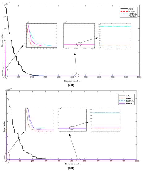
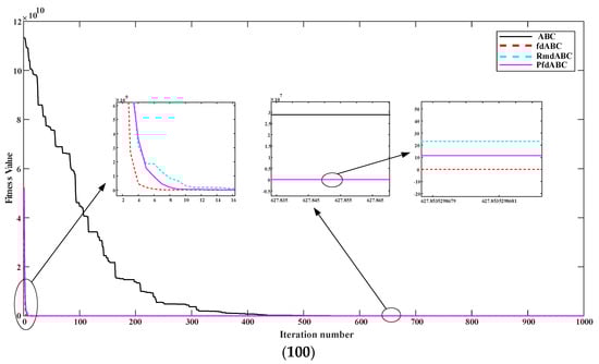
Figure 1.
The fitness values with different strategies for Expanded Schaffer’s Function.
Based on the results above, the introduction of the random multidimensional strategy and parallel full-dimensional strategy greatly improves the performance of traditional ABC. fdABC possesses the best optimization result, but it spends too much time on optimizing. The optimization solutions corresponding to PfdABC and RmdABC are not as good as fdABC, but they can reduce the optimization time effectively. The time cost of RmdABC is lower than fdABC and PfdABC, as RmdABC randomly selects part of dimensions in each iteration. Obviously, the proposed PfdABC and RmdABC algorithms could balance the abilities of exploration and exploitation compared to ABC and fdABC, and the corresponding algorithms must be selected during application on the basis of the practical problems.
4.2. Scheduling Problem
The cargo terminal mentioned in this section is the northern freight area in Xinzheng international airport, and there are totally 16 entrances and exits in total in the container storage area. The coordinates of the nine entrances are R1(1-1-5), R2(2-1-15), R3(1-1-20), R4(1-1-25), R5(1-1-30), R6(1-1-35), R7(1-1-40), R8(1-1-50), and R9(1-1-60), and the coordinates of exits are C1(1-1-8), C2(1-1-18), C3(1-1-28), C4(1-1-38), C5(1-1-48), C6(2-1-53), and C7(1-1-58) respectively, where the first value in the bracket represents the row number of shelf, the second value indicates the number of layers, and the third value is the number of columns. Sixty tasks are waiting to be scheduled, where the first thirty tasks are inbound and the later thirty tasks are outbound. The assigned positions are listed as Table 5.
Table 5.
Task sets to be scheduled.
For solving the optimal scheduled sequence, a sort mapping coding (SMC) strategy is introduced to establish the mapping relationship between the solution and optimization algorithm. It assigns a random number to each dimension of the solution, then sorts the numbers in ascending order and assigns index values based on their sequence. The resulting sequence represented by the index values is the scheduling scheme. The values obtained with SMC could be updated based on Equation (7) with the help of ABC, where the number of dimensions to be updated is determined by different algorithms: ABC algorithm only randomly selects one dimension, all dimensions can be updated in PfdABC, and RmdABC randomly selects certain dimensions.
For the above scheduling problem, comparative studies among five algorithms, including PSO, ABC, PfdABC, and RmdABC, are executed. The scheduling program ran 20 times, and Table 6, Table 7, Table 8 and Table 9 show the optimization results, including the convergence iterations and task execution time corresponding to the optimal solution, the resulting sequences, and the allocation plans of entrances and exits. Obviously, all swarm intelligent algorithms could solve the complicated cargo scheduling problem in certain iterations.
Table 6.
(a) The scheduling results with PSO. (b) Entrances and exits allocation scheme with PSO.
Table 6.
(a) The scheduling results with PSO. (b) Entrances and exits allocation scheme with PSO.
| (a) | ||||||||||
| 1 | 2 | 3 | 4 | 5 | 6 | 7 | 8 | 9 | 10 | |
| Iteration | 889 | 654 | 805 | 841 | 912 | 735 | 889 | 903 | 836 | 749 |
| Result/s | 6841.9 | 6811.9 | 6828.4 | 6779.6 | 6854.9 | 6819.5 | 6841.9 | 6866.1 | 6826.1 | 6811.9 |
| 11 | 12 | 13 | 14 | 15 | 16 | 17 | 18 | 19 | 20 | |
| Iteration | 889 | 654 | 901 | 912 | 912 | 905 | 697 | 903 | 827 | 749 |
| Result/s | 6841.9 | 6811.9 | 6828.4 | 6854.9 | 6854.9 | 6819.5 | 6757.4 | 6866.1 | 6826.1 | 6828.4 |
| (b) | ||||||||||
| Inbound tasks | Outbound tasks | |||||||||
| 1 | 4, 27, 25, 30, 26, 7, 15, 24, 2, 16, 17, 11 | 1 | 39, 40, 51, 45, 60, 34, 38, 44, 31, 46, 33, 59, 41 | |||||||
| 2 | 1, 5, 12, 14, 21, 10 | 2 | 52, 53, 58,3 6, 35, 55, 42 | |||||||
| 3 | 9 | 3 | 47, 54, 56, 43, 49 | |||||||
| 4 | 29, 8 | 4 | 32, 48 | |||||||
| 5 | 19 | 5 | 37 | |||||||
| 6 | 23 | 6 | ||||||||
| 7 | 13, 22, 28 | 7 | 57, 50 | |||||||
| 8 | 18, 3, 20, 6 | |||||||||
Optimal scheduling route: 39 40 4 51 1 45 60 27 34 25 38 30 26 13 18 57 50 3 23 32 48 29 5 44 7 31 12 14 15 24 46 2 33 59 16 17 41 52 9 47 21 53 58 10 36 35 55 8 19 22 28 20 54 56 37 6 43 49 42 11.
Table 7.
(a) The scheduling results with ABC. (b) Entrances and exits allocation scheme with ABC.
Table 7.
(a) The scheduling results with ABC. (b) Entrances and exits allocation scheme with ABC.
| (a) | ||||||||||
| 1 | 2 | 3 | 4 | 5 | 6 | 7 | 8 | 9 | 10 | |
| Iteration | 1098 | 872 | 725 | 915 | 1003 | 1000 | 697 | 605 | 835 | 898 |
| Result/s | 6852.9 | 6772.4 | 6806.41 | 6697.15 | 6892.79 | 6905.64 | 6748.78 | 6865.9 | 6787.76 | 6803 |
| 11 | 12 | 13 | 14 | 15 | 16 | 17 | 18 | 19 | 20 | |
| Iteration | 732 | 1079 | 509 | 840 | 602 | 675 | 786 | 821 | 753 | 835 |
| Result/s | 6839.3 | 6824.9 | 6877.64 | 6796.28 | 6787.27 | 6864.15 | 6808.01 | 6871.29 | 6839.52 | 6817.27 |
| (b) | ||||||||||
| Inbound tasks | Outbound tasks | |||||||||
| 1 | 17, 25, 10, 16, 11, 15, 27, 26, 7, 24, 4, 30, 2 | 1 | 34, 33, 51, 60, 40, 45, 44, 39, 38, 41, 31, 46, 59 | |||||||
| 2 | 14, 21, 12, 1, 5 | 2 | 52, 36, 55, 35, 54, 53, 42, 58 | |||||||
| 3 | 9 | 3 | 56, 49, 43, 47 | |||||||
| 4 | 8, 29 | 4 | 32, 48 | |||||||
| 5 | 19 | 5 | 37 | |||||||
| 6 | 23 | 6 | ||||||||
| 7 | 22, 28, 13 | 7 | 57, 50 | |||||||
| 8 | 20, 18, 3, 6 | |||||||||
Optimal scheduling route: 17 34 25 14 33 51 10 9 22 60 16 52 36 11 15 27 40 19 55 56 45 26 23 44 7 39 21 38 24 35 41 4 30 12 20 18 3 1 54 28 49 43 53 37 8 31 42 47 32 2 6 46 48 13 57 5 59 50 58 29.
Table 8.
(a) The scheduling results with PfdABC. (b) Entrances and exits allocation scheme with PfdABC.
Table 8.
(a) The scheduling results with PfdABC. (b) Entrances and exits allocation scheme with PfdABC.
| (a) | ||||||||||
| 1 | 2 | 3 | 4 | 5 | 6 | 7 | 8 | 9 | 10 | |
| Iteration | 488 | 230 | 223 | 501 | 179 | 346 | 267 | 464 | 202 | 595 |
| Result/s | 6621.11 | 6623.11 | 6613.61 | 6609.98 | 6617.36 | 6617.24 | 6617.36 | 6611.73 | 6617.12 | 6615.49 |
| 11 | 12 | 13 | 14 | 15 | 16 | 17 | 18 | 19 | 20 | |
| Iteration | 213 | 464 | 228 | 82 | 82 | 536 | 153 | 524 | 422 | 388 |
| Result/s | 6606.35 | 6617.48 | 6630.49 | 6615.37 | 6611.86 | 6617.36 | 6617.48 | 6619.24 | 6615.37 | 6611.74 |
| (b) | ||||||||||
| Inbound tasks | Outbound tasks | |||||||||
| 1 | 15, 16, 24, 25, 17, 7, 11, 26, 4, 30, 2 | 1 | 46, 31, 41, 45, 44, 59, 38, 33, 60, 51, 34, 39, 40 | |||||||
| 2 | 14, 12, 5, 1, 10, 21 | 2 | 55, 42, 35, 58, 52, 36, 53 | |||||||
| 3 | 9 | 3 | 54, 56, 47, 43, 49 | |||||||
| 4 | 29, 27 | 4 | 32, 48 | |||||||
| 5 | 19 | 5 | 37 | |||||||
| 6 | 23 | 6 | ||||||||
| 7 | 13, 28 | 7 | 57, 50 | |||||||
| 8 | 18, 6, 3, 20, 8, 3 | |||||||||
Optimal scheduling route: 15 16 46 31 24 41 55 42 54 56 29 25 45 27 44 14 35 58 9 47 43 49 19 23 32 13 28 22 37 18 6 3 57 50 20 48 8 59 17 38 33 12 52 7 11 60 51 34 39 5 1 36 10 53 21 26 4 30 40 2.
Table 9.
(a) The scheduling results with RmdABC. (b) Entrances and exits allocation scheme with RmdABC.
Table 9.
(a) The scheduling results with RmdABC. (b) Entrances and exits allocation scheme with RmdABC.
| (a) | ||||||||||
| 1 | 2 | 3 | 4 | 5 | 6 | 7 | 8 | 9 | 10 | |
| Iteration | 209 | 209 | 213 | 209 | 223 | 546 | 580 | 209 | 331 | 423 |
| Result/s | 6617.12 | 6617.12 | 6611.86 | 6617.12 | 6611.86 | 6611.86 | 6615.61 | 6617.12 | 6617.24 | 6617.36 |
| 11 | 12 | 13 | 14 | 15 | 16 | 17 | 18 | 19 | 20 | |
| Iteration | 539 | 191 | 209 | 223 | 529 | 580 | 546 | 223 | 209 | 223 |
| Result/s | 6621.11 | 6611.86 | 6617.12 | 6611.86 | 6615.61 | 6615.61 | 6615.61 | 6611.86 | 6617.12 | 6611.86 |
| (b) | ||||||||||
| Inbound tasks | Outbound tasks | |||||||||
| 1 | 15, 11, 30, 27, 7, 26, 24, 25, 17, 2, 16, 4 | 1 | 39, 59, 34, 38, 41, 40, 31, 60, 33, 45, 51, 46, 44 | |||||||
| 2 | 21, 14, 12, 1, 10, 5 | 2 | 52, 42, 58, 36, 53, 55, 35 | |||||||
| 3 | 9 | 3 | 47, 54, 49, 43, 56 | |||||||
| 4 | 29, 8 | 4 | 48, 32 | |||||||
| 5 | 19 | 5 | 37 | |||||||
| 6 | 23 | 6 | ||||||||
| 7 | 13, 22, 28 | 7 | 57, 50 | |||||||
| 8 | 20, 3, 6, 18 | |||||||||
Optimal scheduling route: 15 39 59 21 52 14 11 30 27 34 38 41 40 7 26 31 46 44 12 42 9 47 19 29 8 58 1 36 54 49 48 13 22 37 20 3 57 50 6 18 28 32 23 10 24 25 17 60 2 33 45 5 53 16 4 51 55 35 43 56.
The statistical information of the above results are described in the box plot as Figure 2. The numbers 1, 2, 3, and 4 in horizontal coordinate represent PSO, ABC, PfdABC, and RmdABC, respectively. The plot shows that PfdABC and RmdABC are better as the upper limits are lower than the lower limits of PSO and ABC, PfdABC possesses higher optimization accuracy because of its lower low limit, and RmdABC is more stable as the distance between the lower and upper limits is shorter.
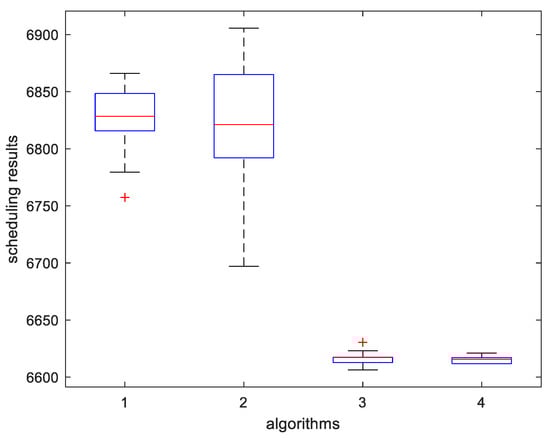
Figure 2.
Box plot of corresponding algorithms.
In addition, several important indices, including the average time required to execute the resulting sequence (Avg), the shortest executed time (Min), the longest inbound and outbound time (Max), and the average convergence generations (Ite) are calculated based on the results of 20 independent runs and shown in Table 10. It can be easily found that the minimum, maximum, and average inbound and outbound time corresponding to PfdABC and RmdABC decreased by 4% at most compared to conventional ABC and PSO, and there are relatively small gaps among the values of Avgs. On the other hand, by examining the values of Ite, it can be seen that PfdABC and RmdABC require less generations to locate the optimal solutions and that it improves by almost 60% compared to ABC and PSO, that is, the advantage of fast convergence speed could be proved.
Table 10.
The scheduling results.
Therefore, PfdABC and RmdABC can obtain faster convergence speed and smaller mean values than those of ABC and PSO in the scheduling problem, and they are demonstrated to be useful tools for solving the air cargo terminal scheduling problem.
5. Conclusions
To improve the efficiency of the cargo terminal in a smart transport system, the intelligent ABC algorithm was introduced to schedule the task set in this paper. Moreover, for increasing the diversity of the population while accelerating the convergence, improved algorithms, including PfdABC and RmdABC, are proposed to enhance the optimization performance. The experimental results show that the ABC, PfdABC, and RmdABC algorithms can solve the task-sets scheduling problem and that the proposed RmdABC and PfdABC algorithms could improve the exploration and exploitation performance efficiently.
The proposed algorithms are efficient in solving complex optimization problems, but their ability of solving dynamic scheduling problems should be verified, and the adaptation of control parameters of ABC for different scheduling requirements should be addressed.
Author Contributions
Conceptualization, H.W. and M.S.; funding acquisition, S.W. and H.W.; investigation and methodology, X.X. and H.W.; supervision, Y.W.; writing—original draft, H.W., Y.W., H.-D.H. and R.Z.; writing—review and editing, H.W., H.-D.H. and S.W. All authors have read and agreed to the published version of the manuscript.
Funding
This research was funded by the Training Program for Young Teachers in Universities of Henan Province (No. 2020GGJS137) and the Key Technologies R&D Program of Henan (Nos. 222102210016, 232102211020 and 222102210019).
Institutional Review Board Statement
Not applicable.
Informed Consent Statement
Not applicable.
Data Availability Statement
Data can be obtained from the corresponding author upon reasonable request.
Acknowledgments
The authors would like to thank Ping Liu, Hongjun Li and Jianhua Wei for their valuable discussions and feedback.
Conflicts of Interest
The authors declare no conflict of interest.
References
- Tang, L.C.; Ng, T.S.; Lam, S.W. Improving air cargo service through efficient order release. In Proceedings of the 7th International Conference on Service Systems and Service Management, Tokyo, Japan, 28–30 June 2010. [Google Scholar]
- Wu, P.J.; Yang, C.K. Sustainable development in aviation logistics: Successful drivers and business strategies. Bus. Strategy Environ. 2021, 30, 3763–3771. [Google Scholar] [CrossRef]
- Gong, Q.; Wang, K. International trade drivers and freight network analysis: The case of the Chinese air cargo sector. J. Transp. Geogr. 2018, 71, 253–262. [Google Scholar] [CrossRef]
- Kuhn, H.W. The Hungarian method for the assignment problem. Nav. Res. Logist. Q. 1955, 2, 83–97. [Google Scholar] [CrossRef]
- Hu, W.; Mao, J.; Wei, K. Energy-efficient Dispatching Solution in an Automated Air Cargo Terminal. In Proceedings of the IEEE International Conference on Automation Science and Engineering, Madison, WI, USA, 17–20 August 2013; pp. 144–149. [Google Scholar]
- Hamzaoui, M.A.; Sari, Z. Optimal dimensions minimizing expected travel time of a single machine flow rack AS/RS. Mechatronics 2015, 31, 158–168. [Google Scholar] [CrossRef]
- Boysen, N.; Fedtke, S.; Weidinger, F. Optimizing automated sorting in warehouses: The minimum order spread sequencing problem. Eur. J. Oper. Res. 2019, 270, 386–400. [Google Scholar] [CrossRef]
- Guo, C.H. Research on application of scheduling optimization of ETV based on improved genetic algorithm. Logist. Sci.-Tech. 2015, 38, 61–69. [Google Scholar]
- Qiu, J.D.; Jiang, Z.Y.; Tang, M.N. Research and application of NLAPSO algorithm to ETV scheduling optimization in airport cargo terminal. J. Lanzhou Jiaotong Univ. 2019, 34, 65–70. [Google Scholar]
- Ding, F.; Song, X.J. Application of shared fitness particle swarm in double ETV system. Comput. Meas. Control. 2018, 26, 228–247. [Google Scholar]
- Radhwan, A.A.; Saleh, R.A. Artificial bee colony algorithm with directed scout. Soft Comput. 2021, 25, 13567–13593. [Google Scholar]
- Dokeroglu, T.; Sevinc, E.; Cosar, A. Artificial bee colony optimization for the quadratic assignment problem. Appl. Soft Comput. 2019, 76, 595–606. [Google Scholar] [CrossRef]
- Awadallah, M.A.; Betar, M.A.; Bolaji, A.L.; Doush, I.A.; Hammouri, A.I.; Mafarja, M. Island artificial bee colony for global optimization. Soft Comput. 2020, 24, 13461–13487. [Google Scholar] [CrossRef]
- Roeva, O.; Petkova, D.; Castillo, O. Joint set-up of parameters in genetic algorithms and the artificial bee colony algorithm: An approach for cultivation process modelling. Soft Comput. 2021, 25, 2015–2038. [Google Scholar] [CrossRef]
- Forouzandeh, S.; Berahmand, K.; Nasiri, E.; Rostami, M. A Hotel Recommender System for Tourists Using the Artificial Bee Colony Algorithm and Fuzzy TOPSIS Model: A Case Study of Trip Advisor. Int. J. Inf. Technol. Decis. Mak. 2021, 20, 399–429. [Google Scholar] [CrossRef]
- Li, Y.C.; Liu, L.B.; Wang, J.; Zhao, J. Improved artificial bee algorithm for reliability-based optimization of truss structures. Open Civ. Eng. J. 2018, 11, 235–243. [Google Scholar]
- Luo, K.P. A hybrid binary artificial bee colony algorithm for the satellite photograph scheduling problem. Eng. Optim. 2020, 52, 1421–1440. [Google Scholar] [CrossRef]
- Alazzawi, A.; Rais, H.M.; Basri, S. Hybrid artificial bee colony strategy for t-way test set generation with constraints support. In Proceedings of the IEEE Student Conference on Research and Development, Bandar Seri Iskandar, Malaysia, 15–17 October 2019. [Google Scholar]
- Weidinger, F. Picker routing in rectangular mixed shelves warehouses. Comput. Oper. Res. 2018, 95, 139–150. [Google Scholar] [CrossRef]
- Zhou, J.J.; Yao, X.F. A hybrid artificial bee colony algorithm for optimal selection of QoS-based cloud manufacturing service composition. Int. J. Adv. Manuf. Technol. 2017, 88, 3371–3387. [Google Scholar] [CrossRef]
- Chen, G.; Sun, P.; Zhang, J. Repair strategy of military communication network based on discrete artificial bee colony algorithm. IEEE Access 2020, 8, 73051–73060. [Google Scholar] [CrossRef]
- Ustun, D.; Toktas, A.; Erkan, U.; Akdagli, A. Modified artificial bee colony algorithm with differential evolution to enhance precision and convergence performance. Expert Syst. Appl. 2022, 198, 116930. [Google Scholar] [CrossRef]
- Long, X.J.; Zhang, J.T.; Zhou, K.; Jin, T.G. Dynamic Self-Learning Artificial Bee Colony Optimization Algorithm for Flexible Job-Shop Scheduling Problem with Job Insertion. Processes 2022, 10, 571. [Google Scholar] [CrossRef]
- Xu, F.Y.; Li, H.L.; Pun, C.M.; Hu, H.D. A new global best guided artificial bee colony algorithm with application in robot path planning. Appl. Soft Comput. 2020, 88, 106037. [Google Scholar] [CrossRef]
- Chen, X.; Wei, X.; Yang, G.X.; Du, W.L. Fireworks explosion based artificial bee colony for numerical optimization. Knowl.-Based Syst. 2020, 188, 105002. [Google Scholar] [CrossRef]
- Brajevic, I. A shuffle-based artificial bee colony algorithm for solving integer programming and minimax problems. Mathematics 2021, 9, 1211. [Google Scholar] [CrossRef]
- Wang, H.Q.; Wei, J.H.; Wen, S.J.; Hou, Y.L. Research on parallel optimization of artificial bee colony algorithm. In Proceedings of the International Conference on Advanced Mechatronic system, Auckland, New Zealand, 9–12 July 2018. [Google Scholar]
- Karaboga, D.; Akay, B. A comparative study of Artifificial Bee Colony algorithm. Appl. Math. Comput. 2009, 214, 108–132. [Google Scholar]
Disclaimer/Publisher’s Note: The statements, opinions and data contained in all publications are solely those of the individual author(s) and contributor(s) and not of MDPI and/or the editor(s). MDPI and/or the editor(s) disclaim responsibility for any injury to people or property resulting from any ideas, methods, instructions or products referred to in the content. |
© 2023 by the authors. Licensee MDPI, Basel, Switzerland. This article is an open access article distributed under the terms and conditions of the Creative Commons Attribution (CC BY) license (https://creativecommons.org/licenses/by/4.0/).