Numerical Study on the Influence of Coupling Beam Modeling on Structural Accelerations during High-Speed Train Crossings

Abstract

The applied mechanical modeling of train and bridge structures is essential in accurately predicting structural vibrations caused by high-speed trains, particularly for the often design-relevant structural accelerations. Considering the interaction effects between the train, the superstructure, and the supporting structure yields more realistic and lower acceleration results compared to simplistic reference models disregarding interaction dynamics. The research presented in this article focuses on modeling single-span girder bridges with a ballasted superstructure as coupling beams. In this approach, the bridge is represented as two vertically coupled beams, with one representing the track (rails and sleepers) and the other representing the supporting structure. Their connection incorporates the stiffness and damping properties of the ballasted superstructure, reproducing its load distribution capacity. A numerical study encompassing a wide range of bridge parameters is conducted, focusing on the calculation of maximum structural accelerations. The results from modeling the bridge as a coupling beam model are compared to those from a simply supported Bernoulli–Euler beam. The excitation is applied as either a moving load or a multi-body model of an Austrian Railjet to evaluate the interdependencies of interaction effects between the vehicle and track and between the track and bridge structure. The comprehensive analysis considers varying bridge span, fundamental bending frequency, mass distribution, structural damping, and coupling stiffness and damping properties to identify correlations with the achievable acceleration reduction using the coupling beam model. Compared to the reference model, the coupling beam model can significantly reduce structural acceleration by up to 80%. Reduction levels primarily depend on the coupling stiffness and critical train speed relative to the bridge’s fundamental frequency, with higher fundamental frequency bridges benefiting the most. These findings provide valuable insights for future structure-specific recommendations for adopting the coupling beam and multi-body train models.

1. Introduction

With the growing importance of rail traffic in the existing European railway network and simultaneously increasing axle loads and train speeds, predicting the dynamic behavior of railway bridges under high-speed traffic plays an increasingly important role in assessing bridge structures. The vibrations and subsequent stresses on railway bridges during resonance events, which become relevant with higher train speeds, can often exceed the static loads by many times. Excessive vibrations must be ruled out by computational investigations in existing structures as well as in the design of new infrastructure.

Vertical structural accelerations are normatively limited to 3.5 m/s² by the Eurocode 1990:2002/A1:2005/AC:2010 Appendix A2 [1]. They often become a decisive criterion for operational planning, the design of new bridge structures, or scheduling and the extent of required retrofitting measures on existing bridges. The occurrence of exceedingly high vertical accelerations of the supporting bridge structure may not only impair the riding comfort of passengers by vibrations of the car body that are perceived as unpleasant, but, under certain circumstances, more severe consequences for riding safety can also occur. Possible damage to the supporting structure due to material fatigue is conceivable, as are track failures due to local destabilization of the ballast bed and, as a result, the risk of train derailments.

The dynamic assessment of the large number of existing bridges in the rail network for route approvals of new trains demands straightforward calculation models. Due to the small number of required input parameters, the primarily applied simple models are very suitable when there is a lack of reliable information about the structures and the trains passing over them. Furthermore, they can be transferred into mathematical models for which the equations of motion can be solved computationally with time-step integration methods very efficiently. Easily applicable models are, for instance, described in [2,3,4,5,6,7].

However, comparing in situ measured bridge vibrations and those calculated with straightforward models shows that the mathematically predicted bridge vibrations often significantly overestimate reality [8,9]. Subsequently, proving compliance with the normatively specified limit values for vertical structural accelerations and displacements in serviceability checks according to Eurocode EN 1990/A2 [1] may be hindered, especially in the case of existing structures. Without closer investigation, for example, by measurements, these overly conservative results can lead to substantial operational restrictions (speed restrictions) or even the need for cost-intensive retrofitting measures, impeding the establishment of efficient maintenance strategies for rail infrastructure buildings.

The discrepancy between measurement and calculation is highly topical and complex. It can be traced back to several causes, such as the structural damping or fundamental frequency of existing bridges, which can often only be estimated with uncertainty without more precise measurements. Both parameters are influenced by numerous factors that are still subject to extensive research activities, i.e., the time-dependent and non-linear track and material behavior [10], the track typology [11], the influence of pre-stressed tendons in concrete beams [12,13], or the shear stiffness [14,15] and damping capacity of the ballasted superstructure [16,17].

One essential aspect is the omission of beneficial influences from interaction dynamics in favor of those straightforward calculation models with insufficient modeling depth, which require multiple simplifications in the mechanical modeling of the bridge and the passing train.

1.1. Multi-Body Dynamic Models

The simplest mechanical model assigns all the properties of a bridge structure to one simply supported bending beam (Bernoulli–Euler beam) and idealizes the dynamic excitation from a passing high-speed train as a series of constant static axle loads moving over it (the moving load model). However, this model is highly conservative and often generates large calculated vibration responses, which, in many cases, significantly exceed the vibrations measured on real structures (e.g., in [8,9,18]).

More complex models considering the interaction dynamics between the train masses, superstructure, and supporting structure by implementing multi-body modeling of all elements allow for a more accurate computational prediction of structural vibrations while requiring a higher number of structural or train parameters in the modeling. With this, precise knowledge of coupling properties regarding the train’s suspension stages plays a central role as they significantly influence the calculated vibrations.

A large part of the current research activities on railway bridge dynamics, for instance, described in [4,6,18,19,20,21,22,23], deals with the computational vibration reduction that can be achieved by modeling the train more accurately as a multi-body system and, therefore, including interaction dynamics between the vehicle and bridge components. In practice, however, it is often complicated, if not impossible, to obtain specific information on the technical characteristics of, e.g., the trains’ wheelset and bogie suspensions since they are often kept secret due to economic interests by the vehicle manufacturers. The future introduction and admission of new high-speed trains into the existing European railway network will further aggravate this problem.

Deepening the modeling complexity of the considered bridge structures offers another approach to more realistic calculation results, whereby many different modeling alternatives with different requirements for input parameters are applicable, among others described in [24,25,26,27,28]. The present contribution focuses on the influence of modeling the bridge structures as coupling beams, i.e., by considering them as two vertically coupled beams representing the track (rails and sleepers) and the supporting structure. Both beams are interconnected vertically by continuously distributed Kelvin–Voigt elements, whose stiffness and damping properties reflect those of the ballasted superstructure. The equation of motion of the proposed model (explained in more detail in Equations (A1)–(A34)) is approximated using trigonometric shape functions and solved by numerical time-step integration, whereby the system can be dynamically excited by moving load models as well as multi-body models of the train.

This bridge model has the advantage of requiring only a few additional input parameters compared to the reference model of the Bernoulli–Euler beam while still being computationally highly efficient. At the same time, it allows for taking the load-distributing influence of the ballast bed as well as the energy dissipation mechanisms depending on the relative vertical movements of the track grid and bridge structure into account.

However, identifying and implementing appropriate and realistic model-related dynamic stiffness and damping parameters represents a further problem. According to the current state of research, no closed and mechanically and physically justifiable unit of calculation model and related parameters can be given. The literature references that focus on the effects of track–bridge interaction (e.g., in [24,26,27,28,29,30,31,32,33,34,35,36,37,38,39]) apply various models with different levels of complexity to idealize the many interconnected elements of the supporting structure (usually modeled as a Bernoulli–Euler beam) and the components of the superstructure (rails, sleepers, and ballast bed). The idealized dynamic bridge system can consist of two layers, as in the numerical investigations described in the present contribution in Section 2, but also three or more; see schematically displayed in Figure 1 and, for instance, described in [24,26,27,28,29,30,31,32,33,34,35,36,37,38,39]. The more layers and elements that are included, the more information on the dynamic behavior and interaction of the respective elements is required, which poses a challenge, particularly regarding the complex subject of dynamic ballast bed behavior.

The applied coupling properties k_i and c_i between rails and subsoil (bridge structure) in the various literature, which represent the interconnection of the two-layered structural model, show a significant spread by a factor of 24, respectively, and 77 for damping or stiffness coefficients(the literature data are, for example, compiled in [28]). In addition, the origin of those specific coefficients is rarely documented comprehensibly in the corresponding literature, making a plausibility check more difficult.

1.2. Simplified Model Alternatives

The influence of considering the interaction effects of the track, vehicle, and supporting structure has been investigated by several research activities in the past [4,6,18,19,20,21,22,23,24,25,26,27,28,29,30,31,32,33,34,35,36,37,38,39]. The impact of taking vehicle–bridge interaction into account by multi-body modeling of the passing trains has been shown to be dependent on many different characteristics of considered trains and bridges, mainly the bridge structure’s span, fundamental frequencies, and mass distribution, in relation to the axle distances, masses, and properties of the suspension system of the train cars (amongst others described in [18,20,23]). Research indicates that the vibrations are reduced particularly effectively in the case of resonance excitation of the bridges due to the regularly spaced train axles.

As well as explicitly modeling the vehicle and bridge structure as multi-body systems, it is also possible to consider the beneficial effects of the interaction effects by simplified methods, which is partly specified in the current standards to be applied, namely the Eurocode EN 1991-2:2003/AC:2010 [40]. The vibration-reducing effects from considering vehicle–bridge interaction, which primarily takes place in the primary suspension stage (the coupling of the unsprung wheelset masses and the bogies), can currently be considered by the additional damping method as described in EN 1991-2 [40] chapter 8.7. An additional damping ratio representing the vibration-reducing effects of vehicle–bridge interaction in calculations without explicitly considering those effects (applying the moving load model) may be assigned to the examined bridge structures. The amount of this additional damping is defined in the current specification of the EN 1991-2 [40] as only dependent on the bridge span. However, several recent research activities have revealed considerable discrepancies between the acceleration results calculated with more sophisticated multi-body models of different high-speed trains and the alternative application of the additional damping method [18,19,20,21]. In many cases, the latter leads to a substantial underestimation of vehicle–bridge interaction and, therefore, uneconomical results, while in other cases, the impact is overestimated, producing unsafe results. These investigations indicate the complexity of the topic and its dependency on multiple influencing factors regarding bridge and train properties. As a result, the redesigned EN 1991-2, currently in the drafting process and available as prEN 1991-2:2021 [41], will no longer contain recommendations for additional damping. The ÖBB guideline RW 08.01.04, Appendix 1 [42], to be applied for the dynamic calculation of railway bridges in the Austrian rail network, allows implementing additional damping for train passages of the Railjet dependent upon the bridge’s fundamental frequencies and distinguished by bridge type (concrete and steel structures). It was derived in [22] through numerical investigations on a parametric field of bridges.

The load-distributing effect of the ballast bed can be implemented in calculations on simple beam models of the bridge by distributing the moving axle loads, for example, by applying the normatively specified distribution pattern of 25%–50%–25% in the distance of the sleepers according to EN 1991-2 [40]. The standard recommends this distribution for calculations on bridge structures with small spans below L = 10 m, for which especially pronounced reductions in resulting accelerations can be expected. However, since the actual stiffness properties of the ballast bed under dynamic loading are not comprehensively and experimentally researched, the question of whether alternative distributions might consider the ballast bed behavior more accurately cannot be resolved at the current state.

Both simplified methods according to EN 1991-2 [40] of considering the interaction effects, namely the additional damping method and the load distribution pattern of 25%–50%–25%, were based on numerical investigations performed by the European Rail Research Institute (ERRI) in 1999 [25], which had at the time limited computational capacities and, therefore, a limited range of investigations and multiple simplifications regarding the considered train and bridge modeling and parameters.

1.3. Objectives of Numerical Study

The numerical study on a broad range of bridge parameters described in the following sections aims to extensively investigate the influence of expanding the simplest reference modeling of bridge structures and trains utilizing the Bernoulli–Euler beam and the moving load model by either including track–bridge interaction with a two-layered bridge model and/or vehicle–bridge interaction with multi-body modeling of the train. Section 2 contains a more detailed summary of the fundamental mechanical modeling and the variation in parameters of bridge structures and trains. The evaluation of the results obtained using different modeling alternatives enables the identification of the structural properties for which applying a more sophisticated coupling beam model of the bridge structure significantly influences the maximum accelerations and quantifying that influence. Additionally, it is examined to what extent the influence of the coupling beam modeling depends on the chosen train model.

The analyses demonstrate the potential for obtaining lower acceleration results by considering the load-distributing impact of the ballasted superstructure in coupling beam models (facilitating verification of compliance with normative acceleration limits in EN 1990/A2 [1]). They indicate that the influence of multi-body models of the train, which consider vehicle–bridge interaction, is particularly pronounced for different structures than that of the coupling beam modeling.

These findings open up the possibility of formulating structure-dependent recommendations concerning the targeted application of more complex modeling of the structure (coupling beam model) on the one hand and train (multi-body model) on the other. Thus, they enable a realistic calculational prediction of the structural vibrations independent of vehicle information for the greatest possible share of structures.

2. Materials and Methods

A computational parameter study is carried out with a locomotive-hauled Railjet over a wide range of realistic combinations of single-span girder bridge characteristics. The calculation results regarding maximum vertical structural accelerations at midspan during a train passage are subsequently compared with the ones of a simple reference beam model. The applied mechanical idealization of four models with and without vehicle–bridge, and track–bridge interaction is graphically displayed in Figure 2 and summarized in the following sections.

2.1. Mechanical Models of the Bridge Structures

As previously mentioned, the reference model of the bridge used in the following investigations is a simply supported single-span shear-rigid bending beam, referred to as the Bernoulli–Euler beam (see Figure 2a at top). It is characterized by only four parameters: the span L [m], bending stiffness EI [Nm²], mass per unit length μ [kg/m], and Lehr’s damping ratio ζ [%]. Its fundamental frequency n₀, which is varied in the parameter study described in the following sections, can be recalculated from these four fundamental parameters (amongst many, given in [43]):

$$n_0=\frac{\pi }{2 L2}\sqrt{\frac{EI}{\mu }}.$$

(1)

Only lateral deformations in the vertical direction (bending deformations w(x,t)) are considered; longitudinal, lateral, and torsional vibrations are omitted.

The equation of motion (see Equation (A1) and further) can be derived using modal analysis, utilizing the first three modal functions (i = 1, 2, 3) of the form φ_i = sin (iπx/L) as shape functions for the discretization of the bending deformation, as they are expected to govern the maximum vibration response, as, for instance, the investigations in [5,44,45] indicate, and to be sufficient for realistic representation in most cases. The damping matrix of the system is obtained by applying Rayleigh damping with ζ₁ = ζ₂ = ζ. Further information on the derivation of the system of equations of motion can be found, among others, in [7].

The multi-body modeling of the bridge structure (Figure 2a bottom) consists of two vertically coupled beams, the lower one representing the supporting structure (with the properties L_s, E_sI_s, μ_s, and ζ_s) and the upper beam the rails (with the properties L_r, E_rI_r, μ_r, and ζ_r). Both beams are vertically coupled by Kelvin–Voigt elements assuming linear spring stiffness $k_{ba}$ and viscous damping $c_{ba}$. As mentioned in Section 1, these coupling coefficients holistically represent the properties of the ballast bed, including the contributions of the ballast itself, sub-ballast mats, elastic sleeper sole pads, sleeper fasteners, and rail pads.

The beam representing the rails is being prolonged beyond the bearings of the beam representing the supporting structure into the embankment over a length L_emb = (L_r − L_s)/2. This embankment area, where the rail beam is coupled to a rigid subsoil, prevents a sudden impulse excitation of the supporting structure initiated by excessive deformations close to the rail beam bearings that can occur due to the sudden change in subsoil stiffness.

In order to make calculations with the different bridge models comparable, the properties of the overall bridge assigned to the Bernoulli–Euler beam have to be allocated to both beams of the coupling beam model. The mass distribution corresponding to the mass contribution of the ballast bed is allocated to the supporting structure beam μ_s, while the discrete sleeper masses are smeared and allocated to the rail beam μ_r. The bending stiffness of the rail beam is derived from the properties of the two rails (assumed 60E1 profiles), and its damping ratio is assumed to be zero (ζ_r = 0).

The mathematical discretization of this dynamical model for its numerical solution can be performed using, for example, finite bar elements with Hermitian shape functions of the third or fourth order, as described, among others, in [35]. However, this approach has the disadvantage of requiring a high number of bar elements to simulate the beam vibrations accurately, especially in cases where the bending stiffness of the rail beams is substantially lower than that of the supporting structure. The subsequent high number of degrees of freedom results in high demands for computational capacities. In contrast, discretizing the system by applying trigonometric shape functions of both beams leads to calculation results that converge at comparably low degrees of freedom associated with short computation times. The latter approach is extensively described, for example, in [46]. Since the trigonometric shape functions represent the modal functions in the case of two uncoupled beams, this approach can be degenerated to represent the Bernoulli–Euler beam if the input parameters are set accordingly. In the following evaluations, the number of shape functions N_s for the supporting structure beam is kept at three (i_s = 1, 2, 3) as in the calculations for the uncoupled Bernoulli–Euler beam, while the number of shape functions for the rail beam i_r = 1, 2, …, N_r is dependent on the required accuracy of the rail beam vibrations. Regarding the influence of the number of shape functions N_r on the accuracy of the predicted vibrations of the supporting structure, previous investigations and the analyses in [46] concluded that those converge if a minimum natural frequency n_r,lim of the rail beam is considered. This leads to a minimum number of considered shape functions N_r of the rail beam according to the following limitations in dependency on the uncoupled rail beam’s fundamental frequency n_0,r, as follows:

$$n_{N_r,r}>n_{r,lim},$$

(2)

where $n_{N_r,r}$ can be written as follows:

$$n_{N_r,r}=N_r^2 \underset{n_{0,r}}{\underbrace{\frac{\pi }{2 L_r^2}\sqrt{\frac{E_r{I}_r}{{\mu }_r}}}}=N_r^2 n_{0,r}.$$

(3)

With Equation (2), this leads to the following:

$$N_r\ge \sqrt{\frac{n_{r,lim}}{n_{0,r}}}=N_{r,lim}$$

(4)

with $n_{r,lim}$ = 200 Hz (chosen according to preliminary investigations).

The system of equations of motions is subsequently derived by applying the trigonometric shape functions to approximation methods according to Ritz and Galerkin (analogously to the approach for the Bernoulli–Euler beam) and including coupling terms in the stiffness and damping matrices of the system. In order to implement the different beam lengths into the coupling terms, it is necessary to assume discrete coupling of subsoil and rail at a limited number of points along the rail’s longitudinal x-axis with a distance of e and transform the continuous coupling properties ${\overline{k}}_{ba}$ and ${\overline{c}}_{ba}$ to $k_{ba}={\overline{k}}_{ba}/e$ and $c_{ba}={\overline{c}}_{ba}/e$. In the following calculations, a continuous coupling is simulated by adjusting this distance very shortly to e = 0.01 m. Another possibility would be to use the actual sleeper distance of e = 0.6 m, which, according to preliminary investigations, has a negligible influence on the results of medium- to long-span bridges. In very short-span bridges, however, it is possible to obtain slightly different results depending on the number and location of the sleepers on the bridge structure if the ratio of bridge span to sleeper distance becomes too small. Thus, the sleeper distance is set to a minimal value of e = 0.01 m for better comparability.

2.2. Mechanical Models of the High-Speed Train

Both bridge models require the implementation of an external force vector as excitation, which can be obtained by applying different train models.

The moving load model (MLM) is the first train model utilized in the following investigations and is the simplest one applicable (see Figure 2b top). It idealizes the train as a series of static axle loads, F_stat,j, moving with a constant speed v and distances over the bridge model. It can be easily implemented as a generalized force vector in the equation of motion of the bridge by performing a modal transformation with the shape functions φ_i of either the total bridge (Bernoulli–Euler beam i = 1, 2, 3) or the rail (coupling beam i = i_r = 1, 2, …, N_r) evaluated at the respective contact points of each load.

This train model considers no interaction effects between the train and the subsoil, respectively, or the bridge structure. In order to evaluate the impact of these interactions, it is necessary to model the train as a system of coupled masses, for instance, by applying the detailed interaction model (DIM) consisting of the interconnected rigid masses of the car bodies, bogies, and wheelsets (see Figure 2b bottom). The coupling properties reflect the train’s primary and secondary suspensions. Implementing this kind of train model into the dynamic equations requires extending the system of equations of motion of the Bernoulli–Euler beam or the coupled beam by additional degrees of freedom associated with the train masses, particularly the vertical displacements of car bodies, bogies, and wheelsets as well as the car bodies and bogies rotation about the transverse horizontal axis through their center of gravity. The wheelset displacements are equated with bridge deflection, respectively, the rail, at the point of contact, assuming rigid and continuous contact of wheels and rails at all times. This forms the coupling condition of the train and the bridge structure and reduces the vehicle’s degrees of freedom by the displacements of the wheelsets.

The composition of the system matrices necessary to implement the different mechanical models into dynamic calculation programs is summarized in Equations (A1)–(A36) in Appendix A, and was derived by modifying the approach described in [35].

The equations of motion can be solved for the rail and bridge structure beam accelerations, velocities, and deflections by applying numerical time step integration methods for a specific train speed or a range of speeds. All the investigations described in this article were performed using MATLAB [47] scripts, applying the implemented differential equation solver for stiff problems (MATLAB ode15s, see [48]) based on the numerical differentiation formulas (NDFs).

Since the problem is a second-order differential equation problem, it is first traced back to two first-order differential equation problems concerning the first and second derivatives of the displacement and rotational degrees of freedom of the beams representing the supporting structure and track and the train components (vector x, see Equations (A2)–(A6)) with respect to time. The initial values of both equations are chosen as x₀ = 0 and ẋ₀ = 0. The solver integrated in MATLAB includes an automatic choice of the integration time steps, with an output of the results in the time step interval dt = 0.1/v ≤ 0.01 s. All time-dependent system matrices—in the case of the MLM, the shape functions and the load vector as a function of the train’s axle positions, and in the case of the DIM, also the mass, damping, and stiffness matrix of the system—are determined anew for each time step. The relative and absolute error tolerance is selected according to the default settings of the solver with 1 × 10⁻³ and 1 × 10⁻⁶.

2.3. Parametric Analysis—Bridge Parameters

In order to draw valid conclusions regarding the effects of considering track–bridge or vehicle–bridge interactions using the previously described model alternatives on a spectrum of single-span bridge structures representative of reality, calculations were conducted on a broad parameter field of bridges. The varied input parameters were the bridge’s span L, mass distribution μ, Lehr’s damping ratio ζ, and fundamental frequency n₀ according to Equation (1). The limits of the parametric field were obtained by analyzing the characteristics of 275 existing single-span and single-track bridges in the European rail network. Information on their properties was derived from several catalogs of existing bridges, primarily located in Austria, and documented during previous research activities. Additionally, the information on 74 bridges was obtained from the ERRI (European Rail Research Institute) reports RP3 [49] and RP8 [50], on 35 bridges from Frýba [3], and on 25 bridges from Rauert [51], provided these bridges also meet the conditions of being constructed as single-span, single-track structures with ballasted beds.

The bridges are distinguished by their construction type, with 101 steel and 7 composite structures being grouped in the same category as they have similar properties regarding mass distribution and span lengths. The same applies to 99 concrete and 68 filler beam structures. Measured values regarding the fundamental frequencies are available for 104 steel and composite structures and 114 concrete and filler beam structures. For the remaining 57 bridges, fundamental frequencies were recalculated by applying Equation (1) and estimating the bending stiffness EI from the documented cross-sections. Furthermore, not all bridge structures have reliable information on their mass distribution available. Consequently, only the 45 steel and composite structures and 136 concrete and filler beam structures with recorded mass distributions are taken into account for determining this parameter bandwidth. The combinations of span, fundamental frequencies, and mass distribution are graphically represented in Figure 3 and Figure 4.

Figure 3 and Figure 4 also contain the parameter combinations used in the numerical study (marked by small grey, blue, and green circles, respectively). They are obtained by applying regression functions as upper and lower bound limits, which were derived from analyzing the property combinations of the existing bridges by Glatz et al. in [22,52]. The regression functions for the upper and lower bound limits of the span-dependent fundamental frequencies n_0,ub(L) and n_0,lb(L) have been determined in [22] as power functions, as follows:

$$n_{0,ub}=113.1 L^{-0.8312}$$

(5)

$$n_{0,lb}=82.43 L^{-0.9937}$$

(6)

The combinations of parameters for the numerical study were obtained by evaluating Equations (5) and (6) for spans L from 4 to 40 m in 1 m increments and choosing five equidistant fundamental frequencies ranging from n_0,ub(L) to n_0,lb(L). The linear regression functions for the span-dependent mass distributions were differentiated according to the masses of the heavier concrete and filler beam and the lighter steel and composite structures. Three mass distributions per construction type (concrete and filler beam: μ₁ to μ₃ steel and composite: μ₄ to μ₆) were chosen following Equation (7) and the input parameters a and b from

Table 1. Input parameters for Equation (7) according to [22].

	Concrete and Filler Beam Structures			Steel and Composite Structures
	μ1	μ2	μ3	μ4	μ5	μ6
a	0.843	0.7002	0.5584	0.1214	0.1214	0.1214
b	10.45	8.539	6.627	9.5174	5.918	2.1691

. Equation (7) is as follows:

$$\mu =a L+b,$$

(7)

where L is in [m] and μ in [t/m].

The Lehr’s damping ratio of the bridges examined was chosen according to the standard EN 1991-2 [40], which must be currently applied. The given span-dependent values also differentiate between reinforced concrete and filler beam structures and steel and composite structures.

$$\begin{array}{cc}\hfill \mathrm{Concrete\; and\; filler\; beam\; structures}:\hspace{1em}\hspace{1em}& \hfill L<20 m: \zeta =1.5+0.07 \left(20-L\right)\hfill \\ & \hfill L\ge 20 m: \zeta =1.5 \hfill \end{array}$$

(8)

$$\begin{array}{cc}\hfill \mathrm{Steel\; and\; composite\; structures}:\hspace{1em}\hspace{1em}& \hfill L<20 m: \zeta =0.5+0.125 \left(20-L\right)\hfill \\ & \hfill L\ge 20 m: \zeta =0.5 \hfill \end{array}$$

(9)

These values are designed as lower and conservative limits of the structural damping and often underestimate the actual damping ratios measured in situ at structures, as, for instance, observed by Reiterer et al. in [8,9]. It is to be expected that future research on the complex discrepancy between measured and normatively prescribed damping ratios will ultimately lead to a revision of the related standards. To investigate whether the influence of vehicle–bridge and track–bridge interaction is independent of the damping ratio used in calculations, the numerical study was also conducted with the normatively prescribed damping value increased by the factors 1.5 and 2 (ζ₁ = ζ_EC; ζ₂ = 1.5 ζ_EC; ζ₃ = 2.0 ζ_EC).

Additionally, applying the coupling beam requires the definition of coupling properties reflecting the ballast bed under dynamic excitation. The approach to modeling the coupling in this article is based on combining all the coupling properties of the ballasted superstructure, i.e., all the individual elements, such as the rail fasteners, intermediate layers, sleepers, sleeper sole pads, the sub-ballast mats, and the ballast bed itself, into a single coupling element with linear stiffness and viscous damping characteristics. The literature references dealing with this modeling show a significant scattering of both coefficients, namely the ballast bed stiffness ${\overline{k}}_{ba}$ and damping ${\overline{c}}_{ba}$ per unit length. The scattering of the literature values was, among others, documented by Stollwitzer in [28] (see Figure 5), which also displays the literature values for three- and four-layer models, including the stiffness and damping properties of the rail fasteners and pads (index rp—rail pads) and/or of the sub-ballast mat (index sb).

Since experimentally determined and verified values are scarce, the impact of applying different stiffness and damping values is investigated by varying these properties as follows:

• Linear stiffness: ${\overline{k}}_{ba,1}$= 50,000 kN/m², ${\overline{k}}_{ba,2}$= 100,000 kN/m², ${\overline{k}}_{ba,3}$= 200,000 kN/m².
• Viscous damping: ${\overline{c}}_{ba,1}$= 30 kNs/m², ${\overline{c}}_{ba,2}$= 60 kNs/m², ${\overline{c}}_{ba,3}$= 100 kNs/m².

In total, 37 different bridge spans from 4 to 40 m with 5 fundamental frequencies each were considered in the following study. Therefore, all calculations on the 185 spans and fundamental frequency combinations were performed for 6 different mass distributions and 3 different structural damping ratios, leading to 3330 parameter combinations for the reference modeling alternative (V1-B1, see Section 2.5). The calculations with the coupling beam model excited by the MLM are performed for a total of five combinations of ${\overline{k}}_{ba}$ and ${\overline{c}}_{ba}$ (${\overline{k}}_{ba,1}$ + ${\overline{c}}_{ba,2}$, ${\overline{k}}_{ba,2}$ + ${\overline{c}}_{ba,2}$, ${\overline{k}}_{ba,3}$ + ${\overline{c}}_{ba,2}$; ${\overline{k}}_{ba,2}$ + ${\overline{c}}_{ba,1}$, and ${\overline{k}}_{ba,2}$ + ${\overline{c}}_{ba,3}$), thus, in total, 16 650 parameter combinations are investigated. Preliminary results showed only a marginal influence of varying the ballast damping coefficient ${\overline{c}}_{ba}$ and the structural damping ζ on the effects of applying the coupling beam model (which will be confirmed by the numerical study, see Section 3.2.3). In order to limit the computational expenses for the most demanding model (coupling beam model and DIM), only the variation in ${\overline{k}}_{ba}$ is investigated with this modeling alternative (${\overline{k}}_{ba,1}$, ${\overline{k}}_{ba,2}$, and ${\overline{k}}_{ba,3}$ in combination with ${\overline{c}}_{ba,2}$ and ζ₁ = ζ_EC → 3330 parameter combinations).

Not all combinations of bridge parameters are equally likely to occur in reality. For instance, steel constructions are usually applied for single-span bridges with higher spans and are simultaneously characterized by a low mass distribution. In order to draw reliable conclusions on the practical benefit of the different modeling alternatives, the results on the parametric field were evaluated while taking the statistical probability of each combination into account. This probability was determined as a multivariate normal probability density function, which can be calculated utilizing pre-implemented functions in MATLAB [47] based on the theoretical description by Kotz et al. in [53]. With this, the documented properties regarding bridge span L, fundamental frequency n₀, and the mass distribution μ served as input parameters, whereby the reciprocal of the span was used to reflect the non-linear relation of span and fundamental frequency. Furthermore, the structural types of concrete and filler beam structures and steel and composite structures were distinguished by performing two separate analyses with the corresponding bridge catalogs.

The matrices of mean values $\overline{m}$ (not to be confused with the mass distribution μ), and covariance Σ are as follows:

$$\overline{m}=\left[\begin{array}{c}\overline{\frac{1}{L}}\\ \overline{\mu }\\ {\overline{n}}_0\end{array}\right], \Sigma =\left[\begin{array}{ccc}{\sigma }_{\frac{1}{L}}^2& {\sigma }_{\frac{1}{L} \mu }& {\sigma }_{\frac{1}{L} n_0}\\ {\sigma }_{\mu \frac{1}{L}}& {\sigma }_{\mu }^2& {\sigma }_{\mu n_0}\\ {\sigma }_{n_0\frac{1}{L}}& {\sigma }_{n_0 \mu }& {\sigma }_{n_0}^2\end{array}\right]$$

(10)

$$\begin{gathered} \mathrm{Concrete\; and\; filler\; beam\; structures}: \\ \overline{m}=\left[\begin{array}{c}0.0939\frac{1}{\mathrm{m}}\\ 17 458\frac{\mathrm{kg}}{\mathrm{m}}\\ 10.115\frac{1}{\mathrm{s}}\end{array}\right], \Sigma =\left[\begin{array}{ccc}0.0019{\left(\frac{1}{\mathrm{m}}\right)}^2& -146.6 \left(\frac{\mathrm{kg}}{{\mathrm{m}}^2}\right)& 0.209\frac{1}{\mathrm{ms}}\\ & 34 274 000 {\left(\frac{\mathrm{kg}}{\mathrm{m}}\right)}^2& -18 509\frac{\mathrm{kg}}{\mathrm{ms}}\\ sym.& & 30.6{\left(\frac{1}{\mathrm{s}}\right)}^2\end{array}\right] \end{gathered}$$

(11)

From the first component in $\overline{m}$ follows $\overline{L}=$10.654 m.

$$\begin{gathered} \mathrm{Steel\; and\; composite\; structures}: \\ \overline{m}=\left[\begin{array}{c}0.0655\frac{1}{\mathrm{m}}\\ 7 451\frac{\mathrm{kg}}{\mathrm{m}}\\ 8.115\frac{1}{\mathrm{s}}\end{array}\right], \Sigma =\left[\begin{array}{ccc}0.00083{\left(\frac{1}{\mathrm{m}}\right)}^2& -22.4 \left(\frac{\mathrm{kg}}{{\mathrm{m}}^2}\right)& 0.101\frac{1}{\mathrm{ms}}\\ & 19 471 000 {\left(\frac{\mathrm{kg}}{\mathrm{m}}\right)}^2& -6 088\frac{\mathrm{kg}}{\mathrm{ms}}\\ sym.& & 15.3{\left(\frac{1}{\mathrm{s}}\right)}^2\end{array}\right] \end{gathered}$$

(12)

From the first component in $\overline{m}$ follows $\overline{L}=$15.261 m.

This information can be utilized to calculate a probability value for each combination of span, mass distribution, and fundamental frequency of the parametric field. A graphical representation of these probabilities is displayed in Figure 6.

It can be observed in Figure 6 that, based on the information on existing bridges available to the authors, concrete and filler beam structures tend to have a high or medium mass distribution (μ₁ or μ₂), spans between L = 6 and 25 m, and corresponding fundamental frequencies of n₀ = 4 to 18 Hz. Steel and composite structures usually have a lighter mass distribution (mainly μ₅), longer spans of L = 9 to 40 m, and, subsequently, lower fundamental frequencies of n₀ = 2 to 14 Hz. Hence, the influence of different modeling alternatives on these most probable combinations of structural parameters will be reviewed in more detail in the following sections.

2.4. Parametric Analysis—Train Parameters

The investigated train in this paper is a locomotive-hauled Austrian Railjet in the standard configuration, which consists of seven regular passenger cars (index pc) and one front locomotive (index loc) with higher axle loads and differing axle distances. In reality, the individual passenger cars feature slightly different characteristics due to their function (i.e., the onboard restaurant) and their position in the configuration. These deviations are considered negligible in the present investigations. Thus, all seven cars are modeled with the parameters of a standard middle car. The train parameters are taken from [4] and are summarized in

Table 2. Train parameters of the Railjet [4].

	Locomotive (loc)	Passenger Car (pc)
Axle load Fstat [kN]	215.6	148.4
Car body mass mc [kg]	51,500	47,316
Car body moment of inertia Ic [kgm]	882 × 103	307 × 104
Bogie mass mb [kg]	13,220	2800
Bogie moment of inertia Ib [kgm]	27,100	1700
Wheelset mass mw [kg]	2495	1900
Length over buffer d [m]	18.59	26.50
Bogie axle distance r [m]	9.90	19.00
Wheelset distance b [m]	3.00	2.50
Primary suspension stiffness kp [kN/m]	3680	1690
Primary suspension damping cp [kNs/m]	80	20
Secondary suspension stiffness ks [kN/m]	2720	280
Secondary suspension damping cs [kNs/m]	200	14

, using the same abbreviations as at the bottom of Figure 2b.

All cars are vertically decoupled from each other, which means that displacements or rotations of individual elements of one car do not affect the adjacent cars. The centers of gravity of all car bodies are assumed to be precisely in the midpoint of the bogie distances, and the centers of gravity of the bogies in the midpoint of the wheelset distances.

2.5. Parametric Analysis—Calculation and Evaluation Parameters

In order to evaluate the effect of considering vehicle–bridge or track–bridge interaction, the accelerations ẅ_max occurring at the structure (either at the Bernoulli–Euler beam or the structural beam of the coupling beam model) are compared with each other in calculations with the different modeling alternatives. The ratio of the maximum accelerations in percent serves as a comparison value, whereby only maximum absolute values during the train crossings in the time domain at midspan are used. In evaluating the acceleration changes $\eta =100\%\frac{{\ddot{w}}_{model}-{\ddot{w}}_{reference}}{{\ddot{w}}_{reference}}$, negative values of η indicate that the maximum accelerations ẅ_reference obtained with a reference model are reduced by the alternative modeling to ẅ_model, while positive values of η indicate an increase in maximum accelerations.

Only peak accelerations are considered, i.e., only local maxima occurring in the defined range of train speeds for which the calculations are performed. Dynamic calculations result in exceptionally high structural vibrations, for instance, peak accelerations, whenever resonance occurs. The acceleration peaks at resonance (generally representing the maximum accelerations within a considered speed range) mainly occur at train speeds at which the regularly spaced train axles exert a periodic excitation close to a natural frequency n_i of the bridge structures. This means that if the train speed is near one resonance speed v_x,i,j according to Equation (13), resonance vibrations are to be expected. Equation (13) is as follows:

$$v_{x,i,j}=\frac{n_i x}{j} ,$$

(13)

where i = 1, 2, …, j = 1, 2, … and x = d, r or b (see Table 2).

In this regard, the length over buffers d_pc of the passenger cars and the fundamental bridge frequency (i = 1) are of particular significance, which means that the highest computational acceleration results are obtained at v_dpc,1,1. The acceleration peak at this critical speed exceeds the accelerations at subordinate resonance scenarios without exception. The Railjet has a maximum operational speed of 230 km/h; however, the calculations for the numerical study were performed for a speed range from 100 to 420 km/h. Since the fundamental frequencies n₀ of the investigated single-span bridges are usually in the range from 2 to 40 Hz, and the passenger car length of the Railjet is d_pc = 26.5 m, the Railjet only reaches the critical speed v_dpc,1,1 within a realistic speed range on a few bridges, for example for the lowest considered fundamental frequency n₀ = 2 Hz at 190 km/h. For most bridge structures, v_dpc,1,1 lies well beyond the operational speed maximum. Subordinate critical speeds at j > 2 most likely produce the critical resonance scenario with the highest acceleration peaks for these bridge structures. The examined speed range was extended to 420 km/h to investigate the effects of considering track–bridge interaction for a representative number of bridge structures at the resonance speed v_dpc,1,1. Thus, all bridge structures with fundamental frequencies below n₀ = 4.4 Hz can reach this particular resonance scenario (48 combinations of span and natural frequency, with spans between 19 and 40 m).

It should be noted that the maximum acceleration occurs at train speeds slightly deviating from v_x,i,j when vehicle–bridge or track–bridge interaction effects are considered. In the case of vehicle–track interaction, the train axle loads rigidly connected to the structure influence their modal mass matrix, which leads to a slight reduction in the natural frequencies and, therefore, the critical speeds at which resonance occurs. In the case of track–bridge interaction, the coupling between the rail beam and the structure beam increases the modal stiffness of the overall bridge, leading to a slight increase in the natural frequencies. Both effects are particularly pronounced in bridge structures with very low mass.

Additionally, another scenario can suppress resonance acceleration peaks: the cancellation effect of bridge vibrations at a specific cancellation speed according to Equation (14):

$$v_{canc,i,j}=\frac{2 n_{0,i} L}{2 j-1},$$

(14)

where i = 1, 2, …, j = 1, 2, …

Resonance effects that might occur at critical speeds v_x,i,j that are close to one only span- and frequency-dependent cancellation speed v_canc,i,j are generally less pronounced or might be suppressed entirely.

All calculations are performed with four different model alternatives, which are referred to as follows:

• V1-B1: Reference calculations with the MLM (V1) and the Bernoulli–Euler beam (B1) → 3330 parameter combinations.
• V2-B1: Calculations with the DIM (V2) and the Bernoulli–Euler beam (B1)—Consideration of vehicle–bridge interaction possible → 3330 parameter combinations.
• V1-B2: Calculations with the MLM (V1) and the coupling beam (B2)—Consideration of track–bridge interaction possible → 16,500 parameter combinations.
• V2-B2: Calculations with the DIM (V2) and the coupling beam (B2)—Consideration of vehicle–bridge and track–bridge interaction possible → 3330 parameter combinations.

The reference calculations with model V1-B1 are performed for the entire speed range in 1 km/h steps. The results are used to identify the highest local acceleration maxima in the chosen speed range, whereby up to five acceleration peaks are considered. The calculations with the other three modeling alternatives considering the interaction effects are performed only for the identified critical speeds with maximum accelerations and a limited speed range around them. This approach helps to significantly reduce the calculation effort for the computationally demanding modeling alternatives V2-B1, V1-B2, and V2-B2. An example can be seen in Figure 7. Acceleration peaks that occur at the boundaries of the overall speed range (close to 100 km/h or 420 km/h) are only included in the following evaluations if all modeling alternatives fully capture them. This prevents distorting the comparison results by shifts of peaks beyond the examination scope due to the increase or reduction in critical speed at which they occur due, as mentioned before, to the modal stiffness or mass increment of the bridges.

3. Results

3.1. Investigation of an Exemplary Bridge Structure

Figure 7 illustrates the speed-dependent acceleration results obtained with the four different modeling alternatives for one exemplary bridge structure representing a light concrete structure (μ₃), which is, in terms of mass distribution, very close to a heavy steel structure (μ₄, see Figure 4). The Lehr’s damping ratio is chosen according to the normative prescriptions in Equation (8). The ballast bed stiffness is ${\overline{k}}_{ba}$ = ${\overline{k}}_{ba,2}$ = 100,000 kN/m² and the damping ${\overline{c}}_{ba}$ = ${\overline{c}}_{ba,2}$ = 60 kNs/m².

In Figure 7, it can be observed that there are three pronounced acceleration peaks in the examined speed range that occur close to v_dpc,1,4 = 410 km/h, between v_dpc,1,8 = 205 km/h and v_dpc,1,7 = 234 km/h, and close to v_dpc,1,11 = 149 km/h. Different acceleration peaks become relevant or decisive depending on which speed range is investigated in bridge verifications under dynamic loading. This is of interest, for example, if lower operational train speeds are prescribed in certain railway sections than the maximum train speed, which may result from other routing conditions (curves, distances to railway stations, etc.). Applying the simplest structural and vehicle model, the Bernoulli–Euler beam and the MLM (V1-B1), leads to the highest acceleration results in all cases. By considering vehicle–bridge interaction (V2-B1), it is possible to obtain lower acceleration results, reduced by η = −2.4% to −12.9%, depending on the respective critical speed at which the acceleration peaks occur. Applying the coupling beam model and, thus, considering track–bridge interaction (V1-B2) leads to a slightly lower reduction in structural accelerations for the peak close to v_dpc,1,4, but a significantly higher reduction in the acceleration peaks at lower critical speeds. The acceleration peak at v_dpc,1,8 is damped by η = −55.9%. The acceleration peak at the even lower resonance speed v_dpc,1,11 is strongly suppressed by applying the coupling beam model so that it no longer appears as a local acceleration maximum in the speed–acceleration curve. If the acceleration at exactly the same speed at which the maximum acceleration peak occurs with the reference model is used for calculating the acceleration reduction η, then it yields a value of η = −80.6%.

Applying the DIM in combination with the coupling beam model (V2-B2) generally yields the lowest acceleration results. The acceleration peak at v_dpc,1,8 is damped to such an extent that the peak at the next higher resonance speed v_dpc,1,7 now slightly exceeds that at v_dpc,1,8 (η = −62.5% compared to the reference acceleration at v_dpc,1,8). With this model alternative, the difference compared to the results of considering only the track–bridge interaction (MLM and coupling beam model V1-B2) is relatively small and of the same order as applying vehicle–bridge interaction to calculations with the Bernoulli–Euler beam. This indicates that applying vehicle–bridge interaction might be relatively independent of the applied structural model. The specific results are summarized in

Table 3. Acceleration peaks and their reduction with different models (reference: V1-B1) of the exemplary bridge structure.

		V1-B1	V2-B1	V1-B2	ηV1-B2/ ηV2-B2	V2-B2
vPeak~vdpc,1,4	Train speed v [km/h]	409	409	413	-	406
	Acceleration ẅmax [m/s2]	13.0	12.7	12.9	-	11.9
	Reduction η [%]	-	−2.4	−1.0	0.12→	−8.6
vPeak~vdpc,1,8/vdpc,1,7	Train speed v [km/h]	209	208	221 **	-	232 **
	Acceleration ẅmax [m/s2]	6.3	5.5	2.8	-	2.4
	Reduction η [%]	-	−12.9	−55.9	0.89→	−62.5
vPeak~vdpc,1,11	Train speed v [km/h]	149	147	149 *	-	149 *
	Acceleration ẅmax [m/s2]	4.0	3.5	0.8	-	0.7
	Reduction η [%]	-	−12.0	−80.6	0.97→	−82.7

* No pronounced acceleration peak recognizable → v_Peak = v_Peak,V1-B1. ** Acceleration peak occurs at different resonance speed → v_Peak > v_Peak,V1-B1.

.

3.1.1. Variation in Coupling Beam Parameters

Figure 8 illustrates the speed-dependent accelerations for the same exemplary structure, but this time with a variation in the structural damping ratio ζ between ζ₁ = ζ_EC (in the case of the exemplary bridge 2.41%) and ζ₃ = 2.0 ζ_EC (4.82%). As expected, higher structural damping yields smaller maximum accelerations, whereby increasing the damping ratio has primarily a scaling effect on the accelerations. By suppressing the most pronounced acceleration peaks, now neighbored peaks may become more relevant in the evaluation of acceleration maxima, as can be observed, for instance, at the peaks at v_dpc,1,11, which are sometimes suppressed with the damping variants ζ > ζ_EC. If no clear acceleration peak can be determined, the acceleration at v_Peak,V1-B1 is used as the comparative value.

The maximum accelerations resulting from applying the reference model V1-B1 and the subsequently calculated reduction values η for the different models and structural damping values are summarized in

Table 4. Acceleration peaks and their reduction with different models (reference: V1-B1) of the exemplary bridge structure with variation in structural damping ζ.

			V1-B1		V2-B1	V1-B2	ηV1-B2/ ηV2-B2	V2-B2
vPeak~vdpc,1,4	ζ1 = ζEC	ẅmax [m/s2]	13.0	η [%]	−2.4	−1.0	0.12→	−8.6
	ζ2 = 1.5 ζEC		9.6		−0.6	0.2	−0.04→	−4.4
	ζ3 = 2.0 ζEC		7.9		−0.2	0.2	0.04→	−4.0
vPeak~vdpc,1,8/vdpc,1,7	ζ1 = ζEC	ẅmax [m/s2]	6.3	η [%]	−12.9	−55.9 **	0.89→	−62.5 **
	ζ2 = 1.5 ζEC		5.3		−6.1	−55.2	0.90→	−61.1
	ζ3 = 2.0 ζEC		4.8		−5.4	−55.9 **	0.93→	−60.0
vPeak~vdpc,1,11	ζ1 = ζEC	ẅmax [m/s2]	4.0	η [%]	−12.0	−80.6 *	0.97→	−82.7 *
	ζ2 = 1.5 ζEC		3.0		−7.7	−75.7 *	0.97→	−77.7 *
	ζ3 = 2.0 ζEC		2.7		−8.1	−73.9 *	0.98→	−75.2 *

* No pronounced acceleration peak recognizable → v_Peak = v_Peak,V1-B1. ** Acceleration peak occurs at different resonance speed → v_Peak > v_Peak,V1-B1. Grey shading indicates approximately equal results

. It can be observed that there is still no significant reduction in accelerations at v_dpc,1,4 when only the coupling beam model or the DIM is applied, independently of the damping ratio. Combining both models yields smaller values of η with an increasing damping ratio. At the second highest resonance scenario at v_dpc,1,8, the influence of the coupling beam model alternative stays approximately the same with increasing damping ratio, while higher damping ratios yield smaller absolute values of η by applying the model V2-B1. The smallest resonance scenario in the examined speed range at v_dpc,1,11 generally produces minor accelerations, especially if the coupling beam is applied. The corresponding values of η also scatter more strongly with the increasing damping ratio than for the other acceleration peaks.

The grey shading of several table elements highlights that the results of η are approximately constant for the same model alternative, independently of the applied structural damping ζ. This especially applies to the influence of implementing the coupling beam model, i.e., to the results of V1-B2 compared to V1-B1 and the results of V2-B2 compared to V2-B1.

Lastly, Figure 9 illustrates the influence of applying different ballast bed stiffnesses ${\overline{k}}_{ba}$ to the coupling beam model and for both vehicle models.

As shown in Figure 9 and the summarized results of η in

Table 5. Acceleration peaks and their reduction with different models (reference: V1-B1) of the exemplary bridge structure with variation in ballast bed stiffness ${\overline{k}}_{ba}$.

			V1-B1		V2-B1	V1-B2	ηV1-B2/ ηV2-B2	V2-B2
vPeak~vdpc,1,4	${\overline{k}}_{ba,1}$	ẅmax [m/s2]	13.0	η [%]	−2.4	−6.4	0.24→	−27.4
	${\overline{k}}_{ba,2}$					−1.0	0.12→	−8.6
	${\overline{k}}_{ba,3}$					1.4	~	0.0
vPeak~vdpc,1,8/vdpc,1,7	${\overline{k}}_{ba,1}$	ẅmax [m/s2]	6.3	η [%]	−12.9	−68.8 **	0.92→	−75.1 **
	${\overline{k}}_{ba,2}$					−55.9 **	0.89→	−62.5 **
	${\overline{k}}_{ba,3}$					−42.3 **	0.85→	−49.8 *
vPeak~vdpc,1,11	${\overline{k}}_{ba,1}$	ẅmax [m/s2]	4.0	η [%]	−12.0	−87.0	0.99→	−87.7 *
	${\overline{k}}_{ba,2}$					−80.6 *	0.97→	−82.7 *
	${\overline{k}}_{ba,3}$					−72.2 *	0.96→	−75.0 *
${\overline{\mathit{k}}}_{\mathit{b}\mathit{a},\mathbf{1}}$ = 50,000 kN/m2; ${\overline{\mathit{k}}}_{\mathit{b}\mathit{a},\mathbf{2}}$ = 100,000 kN/m2$; {\overline{\mathit{k}}}_{\mathit{b}\mathit{a},\mathbf{3}}$ = 200,000 kN/m2

* No pronounced acceleration peak recognizable → v_Peak = v_Peak,V1-B1. ** Acceleration peak occurs at different resonance speed → v_Peak > v_Peak,V1-B1.

, varying the ballast bed stiffness significantly influences the acceleration results, whereby increasing the stiffness leads to higher acceleration results and vice versa. Especially in the case of acceleration peaks at resonances of lower order, such as the peaks occurring at v_dpc,1,8 or v_dpc,1,11, reducing the ballast bed stiffness in calculations with the MLM and the coupling beam model V1-B2 reduces the resulting acceleration peaks much more strongly than additionally including vehicle–bridge interaction by choosing the DIM as the vehicle model. It should also be noted that considering vehicle–bridge interaction is significantly more effective in reducing the acceleration peak at v_dpc,1,4 than at the other resonance peaks, but only if applied simultaneously with the coupling beam model (V2-B2).

In the previous evaluations, the ballast bed damping coefficient was set constant to ${\overline{c}}_{ba}$= ${\overline{c}}_{ba,2}$= 60 kNs/m². The influence of varying this value is examined according to the same principle as the variation in the ballast stiffness. The investigations performed by Bruckmoser in [54] indicate a subordinate influence of the ballast bed damping on the calculated vibrations. For the exemplary structure, the results of reducing the maximum accelerations obtained by varying ${\overline{c}}_{ba}$ while keeping the other structural parameters constant (${\overline{k}}_{ba}$= ${\overline{k}}_{ba,2}$; ζ₁ = ζ_EC) are summarized in

Table 6. Results of acceleration reduction (reference: V1-B1) of the exemplary bridge structure with variation in ballast bed damping ${\overline{c}}_{ba}$.

			V1-B1		V2-B1	V1-B2	ηV1-B2/ηV2-B2	V2-B2
vPeak~vdpc,1,4	${\overline{c}}_{ba,1}$	ẅmax [m/s2]	13.0	η [%]	−2.4	−1.5	0.19	−7.8
	${\overline{c}}_{ba,2}$					−1.1	0.12	−8.6
	${\overline{c}}_{ba,3}$					−1.3	0.15	−8.9
vPeak~vdpc,1,8/vdpc,1,7	${\overline{c}}_{ba,1}$	ẅmax [m/s2]	6.3	η [%]	−12.9	−57.4	0.92	−62.5
	${\overline{c}}_{ba,2}$					−55.9 **	0.89	−62.5 **
	${\overline{c}}_{ba,3}$					−55.6	0.89	−62.7
vPeak~vdpc,1,11	${\overline{c}}_{ba,1}$	ẅmax [m/s2]	4.0	η [%]	−12.0	−80.3	0.97	−82.8
	${\overline{c}}_{ba,2}$					−80.6 *	0.97	−82.7 *
	${\overline{c}}_{ba,3}$					−80.9	0.98	−82.7
${\overline{\mathit{c}}}_{\mathit{b}\mathit{a},\mathbf{1}}$ = 30 kNs/m2; ${\overline{\mathit{c}}}_{\mathit{b}\mathit{a},\mathbf{2}}$ = 60 kNs/m2$; {\overline{\mathit{c}}}_{\mathit{b}\mathit{a},\mathbf{3}}$ = 100 kNs/m2

* No pronounced acceleration peak recognizable → v_Peak = v_Peak,V1-B1. ** Acceleration peak occurs at different resonance speed → v_Peak > v_Peak,V1-B1. Grey shading indicates approximately equal results

. They confirm that only a slight deviation in the calculated acceleration maxima is induced by varying the ballast bed stiffness, which numerical inaccuracies may also explain. Again, the grey-shaded table areas highlight the approximately same results of η for the varied ballast bed damping coefficients.

3.1.2. Evaluation of Critical Train Speed

Based on the evaluations of the results on the exemplary structure described above, it can already be seen what significant influenced not only the modeling, the applied structure, and coupling parameters, but also the considered speed range of the passing trains can have on the results. The latter is particularly relevant because, depending on the respective fundamental frequency of the structure, only certain resonance events can occur in this predefined speed range. However, since the different models can have a different effect on the acceleration results depending on the examined resonance event, not only the reduction in the acceleration by a specific model is investigated in the following evaluations, but also another comparison feature: the maximum speed v_lim at which a prespecified acceleration limit is exceeded for the first time in the calculations applying one of the four models. Subsequently, the normative acceleration limit for railway bridges with ballast superstructure according to EN 1990/A2 [1] is used for this purpose, defined as ẅ_lim = 3.5 m/s².

For the exemplary structure, the resulting values of v_lim are marked in Figure 7, Figure 8 and Figure 9 with yellow markers and shortly summarized for all considered variants of the models and structural parameters in

Table 7. Results of maximum train speed at which ẅ_lim is exceeded for the first time.

ζ	${\overline{\mathit{k}}}_{\mathit{b}\mathit{a}}$	${\overline{\mathit{c}}}_{\mathit{b}\mathit{a}}$		V1-B1	V2-B1	V1-B2	V2-B2
ζ1 = ζEC	${\overline{k}}_{ba,2}$	${\overline{c}}_{ba,2}$	vlim [km/h]	147	147	357	354
ζ2 = 1.5 ζEC				184	188	359	354
ζ3 = 2.0 ζEC				187	189	363	356
ζ1 = ζEC	${\overline{k}}_{ba,1}$	${\overline{c}}_{ba,2}$	vlim [km/h]	147	147	359	354
	${\overline{k}}_{ba,2}$					357	354
	${\overline{k}}_{ba,3}$					205	352
ζ1 = ζEC	${\overline{k}}_{ba,2}$	${\overline{c}}_{ba,1}$	vlim [km/h]	147	147	357	348
		${\overline{c}}_{ba,2}$				357	354
		${\overline{c}}_{ba,3}$				357	354

Grey shading indicates approximately equal results

:

In this comparison, it can be observed that for this exemplary bridge structure, with the application of the coupling beam model, a significant increase in the train speed is achievable, at which the normative acceleration limit according to EN 1990/A2 [1] is reached. Essentially, this effect can be explained by the fact that the resonance events at v_dpc,1,11 and v_dpc,1,8 are suppressed by considering track–bridge interaction to such an extent that they do not generate accelerations of a critical magnitude, so only the resonance event at v_dpc,1,4 becomes relevant.

Between the results with different vehicle models, structural damping ratios, or coupling properties, only marginal results occur, except for the shift of v_lim at the highest ballast bed stiffness ${\overline{k}}_{ba,3}$ to 205 km/h.

3.2. Investigations on a Parametric Field of Bridges

All parameter combinations described in Section 2.3 were investigated analogously to the exemplary bridge, and the results are mainly presented graphically in the following sections.

3.2.1. Acceleration Results of Reference Model

The following Figure 10 shows, for each mass distribution separately, the highest acceleration peak results obtained in the considered speed range when applying the reference model V1-B1. The structural damping ζ for all structures in Figure 10 was set to the normative value ζ₁ = ζ_EC according to Equations (8) and (9). Grey-shaded areas mark those examined bridge structures for which no calculated acceleration exceeded the normative acceleration limit of ẅ_lim = 3.5 m/s² according to EN 1990/A2 [1]. The number of structures for which this is the case increases primarily with increasing mass distribution and bridge span and secondarily with the bridge’s fundamental bending frequency. Within the white dashed contours in each subfigure lie those bridges with parameter combinations with a more than 25%, 50%, or 75% probability of occurrence, according to the investigations in Section 2.3 and Figure 6, distinguished by concrete/filler beam structures and steel/composite structures.

It can be observed that the maximum acceleration peaks for bridge structures with particular spans are significantly lower than for bridges with slightly longer or shorter spans, e.g., for bridges with L = 22 or 23 m. This can be traced back to the occurrence of cancellation effects at the same critical speed at which resonance effects would occur (for example, for L = 22 m: v_dpc,1,3 = n₀ d/3 ≈ v_canc,3 = n₀ 2 L/(2 3-1), see Equations (13) and (14)). This concurrence may oppress the resonance peak so that neighboring but at the same time usually less pronounced resonance peaks become decisive.

Generally speaking, especially the light steel and composite bridges experience exceptionally high accelerations in the considered speed range, which would most likely exceed the normative limitations even at lower train speeds. It should be noted that the absolute acceleration results can only represent fundamental tendencies of the expected dynamic structural response since the results can change significantly when other factors, such as rail irregularities, deviating bearing conditions, or soil–structure interaction, are considered.

3.2.2. Influence of Modeling on Critical Train Speed

As previously mentioned, comparing only maximum peak accelerations yields results strongly dependent on the considered speed range. Thus, Figure 11 displays the train speeds v_lim at which each structure experiences accelerations above the normative limit ẅ_lim = 3.5 m/s² according to EN 1990/A2 [1] for the first time when applying V1-B1. The structural damping of all considered bridge structures in Figure 11 is defined to comply with the normative prescriptions for ζ₁ = ζ_EC. Blue-shaded areas mark parameter combinations for which the train speeds of the Railjet can easily reach 350 km/h or more without causing critical accelerations. However, the graphical representation reveals that especially the bridge structures within the red-shaded areas experience critical accelerations at relatively low train speeds in calculations with V1-B1. Therefore, the basic calculation model could not be applied in the serviceability limit state design for a large share of bridge structures and operational train speeds of 230 km/h.

Applying V2-B1 (the calculation model considering vehicle–bridge interaction effects with the train’s DIM but applying the simple Bernoulli–Euler beam) brings up the critical speed v_lim for many bridge structures, especially the lighter structures with spans L above 15 m, see Figure 12. Conversely, implementing V1-B2 (coupling beam model considering track–bridge interaction and the simple MLM) favorably affects the limit train speeds for shorter bridge structures with spans below 15 m in particular, regardless of the mass distribution, as shown in Figure 13. The graphical representation only contains results obtained with the medium ballast coupling stiffness ${\overline{k}}_{ba,2}$ and damping coefficient ${\overline{c}}_{ba,2}$, but the results for other combinations of ${\overline{k}}_{ba}$ and ${\overline{c}}_{ba}$ display similar tendencies.

Combining both the more sophisticated DIM and the coupling beam model in V2-B2 yields acceleration results for a large share of the considered bridges, which meet the normative acceleration limits at train speeds above 250 km/h and, therefore, above the operational speed of the Railjet, see Figure 14. Both influences observed in Figure 12 and Figure 13 are superimposed, leaving only a few exceptionally light bridges with low fundamental frequencies, which would exceed the acceleration limits at train speeds of less the 200 km/h.

These findings can also be observed in the graphical representation in Figure 15, which displays the percentage of bridge structures with critical accelerations at certain train speeds on an interval scale. Analogous to Figure 11, Figure 12, Figure 13 and Figure 14, the color scale of the figure shows the train speed intervals in which the normative acceleration limit of 3.5 m/s² according to EN 1990/A2 [1] is exceeded for the first time for the concrete and filler beam structures and the steel and composite structures. The stacked bar chart indicates the respective proportion of the bridge structures exceeding said acceleration limit.

At first glance, it is noticeable that it is possible to comply with the acceleration limit without any problems for a large proportion of the concrete and filler beam structures, even at train speeds above 400 km/h, almost irrespective of the dynamic calculation model used. The proportion of structures for which this is not computationally possible at speeds below 250 km/h amounts to a total of 14.9% for the reference model V1-B1 and can be reduced substantially to 5.4% (V1-B2) or, in combination with the DIM (V2-B2), to 3.2%, above all by using the coupling beam model. The use of the DIM without consideration of the track–structure interaction (V2-B1) shows a less pronounced influence on the calculation results.

A more differentiated picture emerges in the case of steel and composite structures, which tend to be associated with lower mass distributions. Generally, the proportion of structures for which verification with the simple reference model V1-B1 becomes problematic is much larger. The acceleration limit is exceeded in about 61.3% of the structures with train speeds below 250 km/h. If the DIM is used alone (V2-B1), the proportion is reduced to 43.5%; if the coupling beam is used alone (V1-B2), it is reduced to 51.9%. The latter, however, has a particularly strong effect on those structures whose maximum acceleration already exceeds the normative limit at 100 to 150 km/h; this proportion is reduced from 31% to 12.4%, while it is still 19.5% when the DIM is used alone.

For both types of structures, the joint application of DIM and coupling beam (V2-B2) is the most influential.

The influence of the different calculation models on the critical train speed v_lim at which the acceleration limit is exceeded is additionally shown in Figure 16. The results are distinguished according to mass distributions μ₁ to μ₆. The resulting bandwidth of v_lim is given for each calculation model, and, furthermore, for the average values, median, and 25% and 75% quartiles. The average, median, and quartiles are also shown as weighted values, whereby the weighting is derived from the probability of structural parameter combinations, as shown in Section 2.3.

Again, this graph shows the tendency for the coupling beam model alone or in combination with the DIM (V1-B2 and V2-B2) to have a more significant effect on the results than using the DIM alone (V2-B1), especially in the observed bandwidth of results. In turn, using the DIM (V2-B1) alone has a stronger effect on the lighter steel structures than using the coupling beam model (V1-B2) alone, whereby a relatively large spread of results can be observed.

3.2.3. Influence of Modeling on Acceleration Peaks

The following graphical evaluations show the reduction in acceleration peaks resulting from applying one of the dynamic calculation models compared to the respective reference model. Figure 17 shows the acceleration reductions η resulting from the sole use of the coupling beam model V1-B2 compared to the reference model V1-B1. Both models are applied to calculations on the parametric field of bridges with the normative structural damping (ζ₁ = ζ_EC), and the coupling beam model assumed medium stiffness and damping (${\overline{k}}_{ba,2}$, ${\overline{c}}_{ba,2}$). The reduction is plotted as a percentage ratio on the ordinate according to the definition given by $\eta =100\%\frac{{\ddot{w}}_{model}-{\ddot{w}}_{reference}}{{\ddot{w}}_{reference}}$. The larger the absolute value of the negative results η, the smaller the resulting acceleration peak when V1-B2 is used compared to the acceleration calculated with V1-B1.

The train speeds at which the respective acceleration peak occurred are plotted on the abscissa in a logarithmic scale. However, these critical speeds are normalized to the respective fundamental frequency n₀ of the structures as follows:

$${\lambda }_{Peak}=\frac{v_{Peak}}{n_0} , v_{Peak} \mathrm{in} [\mathrm{m}/\mathrm{s}]$$

(15)

For each structure, depending on its fundamental frequency and the range of train speeds considered, the calculations were only carried out in specific wavelength ranges of λ. For example, dynamic calculations for a structure with n₀ = 4 Hz are performed for only λ = 27.78 m/s/4 Hz = 6.94 m (lower limit v = 100 km/h) to λ = 116.67 m/s/4 Hz = 29.17 m (upper limit v = 420 km/h). For this exemplary structure, acceleration peaks are to be expected, in particular, at the critical speeds occurring at v_dpc,1,j = d_pc n₀/j (see Equation (13)) or with the relation of Equation (15) in between λ_dpc,1,1 = 26.5 m and λ_dpc,1,3 = 8.83 m.

The evaluation considers one to five acceleration peaks for each structure. The probability that the respective combination of bridge parameters (L, n₀, μ) occurs is characterized by the transparency of the individual markers; the more transparent they are displayed, the less likely the parameter combination is in reality. In addition, the color of the markers gives information about the respective ratio of span L and structural damping ζ of each structure, normalized to the maximum values of the considered parameter field (L_max = 40 m, ζ_max = 2.62%).

Figure 17 reveals a clear dependence of the acceleration reductions η (generated by considering the track–bridge interaction in V1-B2) on the normalized train speed λ at which the respective acceleration peaks occur. The lower the normalized speed λ, the higher the reduction in the respective acceleration, which can take values below −80% for all mass distributions at λ < 2.5 m. In the value range of λ > 10 m, the achievable acceleration reductions approach zero, with a large scatter of results and also positive values of η observed, especially for the steel and composite structures. The more scattered results seem to be related to tendencies of higher values of $\overline{L}$/$\overline{\zeta }$ of the respective structures, i.e., structures with larger spans and, at the same time, low structural damping (particularly frequent in steel and composite structures).

The relationship between λ and η can be approximated by regression functions. The results observed, particularly in the lower value range of λ < 2.5 m, suggest that an s-shaped or sigmoidal regression function would represent the relationship of λ and η better than the exponential regression function of the form, i.e.,:

$$\eta \left(\lambda \right)=\mathrm{a} e^{b \lambda },$$

(16)

as displayed for each mass distribution. However, since a sigmoidal regression function would require considerably more parameters to estimate, the more straightforward exponential form is resorted to, though its validity must be restricted to the range of values 2.5 m < λ < 10 m. The range of the respective parameters a and b to determine the exponential regression functions are given in the legend of Figure 17, as are the coefficients of determination R², which can be understood as a goodness-of-fit measure describing the percentage of the variance in output values that is explained by the variance in input variables (quotient of error squares).

In all subgraphs, the respective regression function and its 95% prediction intervals for new observations are plotted as black solid and dotted lines, respectively. The estimation of parameters for the regression functions according to Equation (16) involved weighting the considered input parameters according to the probability of structural parameter combination estimated in Section 2.3. The weighting factors are supplied as a value between 0 and 1 for each bridge parameter combination, whereby each value corresponds to the probability of occurrence.

The evaluations displayed in Figure 17 could be used to assess the beneficial influence on the maximum acceleration peaks that could be generated by applying the coupling beam model before actually performing the calculations and, therefore, evaluate whether the choice of structural model complexity significantly influences the results. However, this requires prior knowledge of the probable resonance events, or more precisely, the normalized train speed at which particularly pronounced acceleration peaks are most likely to occur. Furthermore, the resulting regression function could be used to estimate the reduction in acceleration obtained with the reference model, even without additional calculations. For this purpose, it would be recommended to use the 95% confidence boundary for new predictions (the upper boundary in Figure 17, illustrated with a dotted line) to ensure sufficient prediction reliability. Since it can be observed that all regression functions regarding the different mass distributions are relatively similar, the parameters for estimating said upper boundary are only given for the regression functions obtained with all calculation results (independent of the respective mass distribution).

Figure 18 shows, analogously to Figure 17, the evaluation of η when the more sophisticated vehicle model DIM is being applied alone (V2-B1) compared to the V1-B1 reference model, again plotted against the normalized train speed λ at which the respective acceleration peaks occur. In contrast to Figure 17, no clear dependence of λ and η can be observed in this plot, although the vehicle model’s influence can take particularly large absolute values of up to η = −70%, especially for acceleration peaks in the range from 6.6 m < λ < 13.2 m. Since much smaller absolute values and positive values of η can occur at the same normalized speeds, specifying a regression function with high predictive reliability is impossible. However, the results indicate that V2-B1 has a more substantial effect with decreasing mass distribution of the structures and that a high ratio of $\overline{L}$/$\overline{\zeta }$ also tends to be associated with larger acceleration reductions η. It is also noticeable that the sole use of the DIM (V2-B1) has a particularly favorable effect at different normalized speeds (λ > 6.5 m) than the sole use of the coupling beam model (V1-B2).

Lastly, Figure 19 shows the influence of using the coupling beam model while simultaneously applying the more complex DIM (V2-B2), but this time in comparison to the reference model V2-B1, i.e., applying the same vehicle model. The figures show a very similar picture to the one already shown in Figure 17, except for a slightly larger scatter of results, which is also reflected in the lower R² values and larger prediction intervals of the determined regression functions. The parameters of the regression functions, especially for the concrete and filler beam structures, are very similar to those obtained by comparing the accelerations obtained with the V1-B2 model with those obtained with V1-B1. The results indicate that the influence of the coupling beam has a very similar effect on the results of the structure accelerations for both vehicle models investigated, namely the MLM (V1) and the DIM (V2).

Figure 20 summarizes the results for comparing the calculation results of models V1-B2 to V1-B1 and models V2-B2 to V2-B1 for all mass distributions. The regression functions created based on all calculation results are shown with solid red lines; the 95% prediction intervals are marked with dashed lines; the respective functions for each mass distribution are displayed as black lines. The mathematical formulation of the overall regression functions can be found in the legend on the right side of the figure. Particularly when comparing the models using the MLM as the vehicle model, there is good agreement between the calculated regression functions of each mass distribution and those calculated based on all results. The boundary line of the upper 95% prediction interval could be assumed to be on the safe side for estimating the achievable acceleration reductions for λ < 8 m.

When using the DIM, it is noticeable that there are more significant deviations of the 95% prediction boundaries of the regression functions for each mass distribution compared to the regression function determined based on all results, in particular for the somewhat lighter mass distributions, whose results noticeably spread more strongly (e.g., μ₆, see Figure 19, right bottom). Nevertheless, both regression functions have high coefficients of determination.

In the example in Section 3.1, it was evident that the applied spring stiffness of the coupling between the rails and the bridge structure ${\overline{k}}_{ba}$, which can also be understood as the dynamic ballast bed stiffness, significantly influences the reduction in the calculated acceleration peaks. This effect can also be seen in the regression functions displayed in Figure 21 for the various coupling stiffnesses investigated, whereby other model parameters (coupling damping coefficient ${\overline{c}}_{ba}$ and structural damping ζ) are kept unchanged. In the center of the figure, the two regression functions already shown in Figure 20 are presented for the models V1-B2 (red) and V2-B2 (green) at the applied medium ballast bed stiffness ${\overline{k}}_{ba,2}$. The left subfigure additionally shows the regression function with the lower ballast bed stiffness ${\overline{k}}_{ba,1}$. This function is shifted to the right compared with ${\overline{k}}_{ba,2}$, which means that if an acceleration peak occurs at the same normalized speed λ, a more significant reduction in the acceleration peak can be expected with lower ballast stiffness. With the higher ballast bed stiffness ${\overline{k}}_{ba,3}$ the determined regression function shifts to the left compared to that with ${\overline{k}}_{ba,2}$, i.e., the acceleration peaks at the same normalized speed are reduced to a lesser extent. This influence of the coupling stiffness can become quite large. For example, the reduction η estimated with the exponential regression function using V1-B2 at λ = 6.625 m (corresponds to v_dpc,1,4) with ${\overline{k}}_{ba,1}$ is about −18.9%, while with ${\overline{k}}_{ba,2}$ it −12.2%, and with ${\overline{k}}_{ba,3}$ it is −7.5%. For acceleration peaks in the range of λ = 4.417 m (corresponds to v_dpc,1,6), the results are η = −45.1%, −33.9%, and −24.1%, respectively.

Furthermore, the subfigure on the left reveals that for the lowest ballast stiffness considered, the results of η obtained with the more complex DIM (green regression functions) differ stronger from those obtained with the MLM (black regression functions), whereby the coupling beam model influences the acceleration results more strongly when it is combined with the more sophisticated vehicle model.

Finally, Figure 22 shows the determined regression functions η(λ) resulting from the analysis of the calculations results when V1-B2 is used versus V1-B1 and other parameters are varied. In the left subfigure, the results yielded from applying different ballast bed stiffnesses ${\overline{k}}_{ba}$ are again displayed, whereby the ballast bed damping coefficients ${\overline{c}}_{ba}$ and the structural damping ζ remain the same for all underlying calculations. The apparent difference in the determined regression functions can also be seen in this diagram. In contrast, increasing or reducing the applied ballast bed damping coefficient ${\overline{c}}_{ba}$ while keeping the other structural parameters constant has no discernible effect on the generated results (see subfigure in the center), nor does increasing the structural damping ζ beyond the normative damping (subfigure on the right).

4. Conclusions and Outlook

Extensive numerical parameter studies are conducted using various models to identify and quantify the influence of four different modeling variants on the calculated structural accelerations. All the model variants share the assumption of relatively straightforward mechanical idealizations and can only capture vibrations in the vertical direction of the structure. In addition to the reference model (V1-B1), which idealizes the structure as a Bernoulli–Euler beam and the vehicle as a series of moving axle loads, two additional models are considered: one (V2-B1) that incorporates vehicle–bridge interaction using a multi-body model of the train (DIM), and another (V1-B2) that accounts for track–structure interaction using a two-layer coupling beam model of the bridge. The last model (V2-B2) combines both interaction effects. A standard configuration eight-car Railjet train is used in all models.

4.1. Statistical Analysis of Bridge Parameters

Four computational models were applied to a parameter field of bridge structures defined by the span (L), mass distribution (μ), fundamental bending frequency (n₀), and structural damping (ζ) of the bridges. The probability of occurrence for combinations of span, mass distribution, and fundamental bending frequency within the parameter field was statistically analyzed using measured or documented structural properties of 275 existing bridge structures (see Figure 3 and Figure 4). This analysis provides a better assessment of the benefits of different modeling variants in terms of their practical relevance in dynamic analyses. The following combinations of structural parameters represent a particularly relevant framework for further investigations (see also Figure 6):

• Regarding existing concrete and filler beam structures, the average span is $\overline{L}$ = 10.65 m, the average mass distribution is $\overline{\mu }$ = 17.5 t/m, and the average fundamental bending frequency ${\overline{n}}_0$ = 10.1 Hz. Combinations with spans ranging from 7 to 23 m and fundamental frequencies from 5 to 17 Hz, particularly for heavy to medium structures (μ₁ to μ₂), have a probability of occurrence greater than 50%.
• Regarding existing steel and composite structures, the average span is $\overline{L}$ = 15.3 m, the average mass distribution is $\overline{\mu }$ = 7.5 t/m, and the average fundamental bending frequency ${\overline{n}}_0$ = 8.1 Hz. Parameter combinations with spans ranging from 10 to 31 m and fundamental frequencies from 4 to 13 Hz, particularly for structures with medium mass distribution (μ₄), have a probability of occurrence greater than 50%.

4.2. Evaluation of Exemplary Bridge Structure

When analyzing the results for the specific exemplary structure (see also Figure 7, Figure 8 and Figure 9 and Table 3, Table 4, Table 5, Table 6 and Table 7), several tendencies emerge that are also confirmed when examining the results of the entire parameter field, as follows:

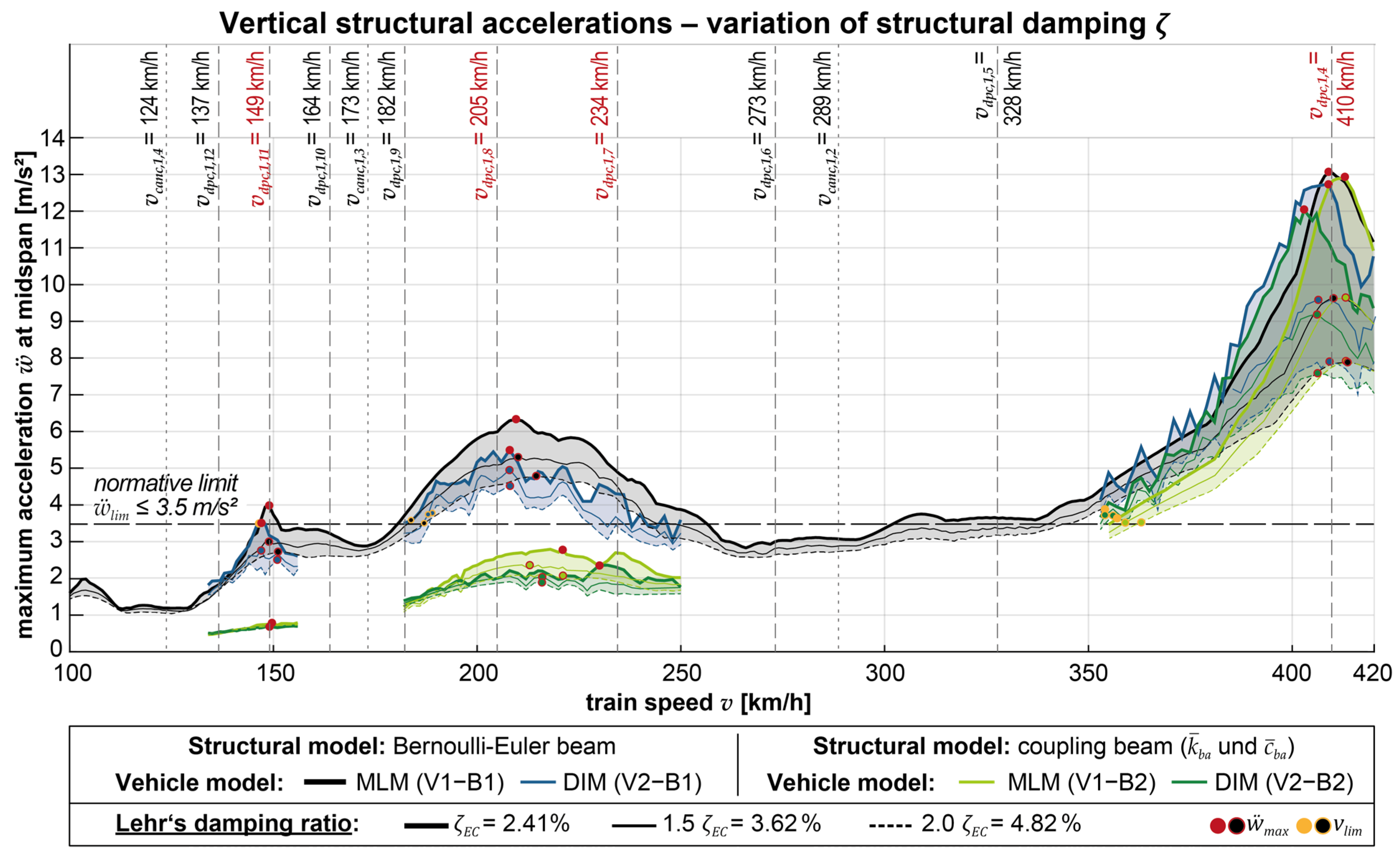
• The reference model (V1-B1) generally yields the highest acceleration values, which can be reduced to varying degrees by using one of the other models. Notably, the most complex model (V2-B2), which considers both track–bridge and vehicle–bridge interaction, consistently produces the lowest accelerations. When assessing the acceleration peak at the maximum train speed, which occurs within the range of the resonant speed v_dpc,1,4 for this specific structure, the most substantial reduction can be achieved by employing the train’s multi-body model (DIM: V2–B1 and V2–B2). However, for acceleration peaks at lower train speeds (v_dpc,1,8 and v_dpc,1,11), the coupling beam model (V1-B2 and V2-B2, respectively) exerts a greater influence in reducing the acceleration results.
• Using the train’s multi-body model alone (V2-B1) leads to a shift in the acceleration peaks towards slightly lower train speeds due to the increase in the modal mass of the overall system caused by considering the train masses. Conversely, employing only the coupling beam model (V1-B2) tends to shift the acceleration peaks towards somewhat higher train speeds. Moreover, the influence of the coupling beam model results in more pronounced damping of acceleration peaks at lower train speeds compared to higher speeds. This effect allows acceleration peaks at higher train speeds, previously overshadowed in the reference model, to become more significant or decisive (see also Figure 9).
• Combining both model extensions in the V2-B2 model reveals an additive superposition of the computational benefits of both interaction effects. Specifically, the accelerations are reduced to a similar extent by applying the coupling beam model, regardless of the vehicle model used (see also Table 3, Table 4, Table 5 and Table 6). This implies that the influence of the coupling beam model on reducing accelerations remains consistent regardless of the specific characteristics of the vehicle model.
• When varying the underlying structural damping ζ (to the same extent in all models), the coupling beam model (V1-B2) demonstrates a similar effect on reducing accelerations (see also Figure 8 and Table 4). However, solely employing the more complex vehicle model (V2-B1) at higher underlying structural accelerations results in a less achievable reduction compared to cases with normatively lower bound damping (ζ₁ = ζ_EC). In other words, the coupling beam model consistently contributes to reducing accelerations regardless of the damping level, whereas the sole application of the more complex vehicle model is less effective in reducing accelerations when the underlying structural accelerations are higher than the normative damping would suggest.
• Varying the coefficients of the ballast bed damping ${\overline{c}}_{ba}$ while using the coupling beam model shows only marginal deviation in the resulting influence on accelerations (see also Table 6). This indicates that the ballast bed damping has no noticeable impact on the influence of the coupling beam model on structural accelerations within the considered range of variation.
• When the spring stiffness of the ballast bed ${\overline{k}}_{ba}$ is varied while utilizing the coupling beam model, a significant influence on computed acceleration reductions is observed (see also Figure 9 and Table 5). Specifically, a lower applied ballast stiffness is associated with a higher reduction in acceleration.
• The evaluation of speeds v_lim, at which the calculated structural acceleration exceeds the acceleration limit of ẅ_max = 3.5 m/s² specified by the standard, reveals a significant potential for the coupling beam model to assess high-speed train crossings as computationally uncritical. For the exemplary structure, regardless of the specific parameters applied to the coupling stiffness ${\overline{k}}_{ba}$, coupling damping ${\overline{c}}_{ba}$, structural damping ζ, and vehicle model (MLM or DIM), the coupling beam model allows for train speeds exceeding 350 km/h without exceeding the acceleration limit (see also Table 7). In contrast, the reference model predicts a first-time exceedance of the acceleration limit at speeds below 150 km/h. Additionally, applying the DIM (V2-B1) alone does not significantly influence the limit speed achieved with the reference model (V1-B1) for this specific exemplary structure.

4.3. Evaluation of Parametric Field of Bridges

The results obtained from the analysis of the entire parameter field confirm the tendencies observed for the exemplary structure and provide the basis for deriving some fundamental conclusions. The evaluation focuses on examining the specific impact of the extended models (V2-B1, V1-B2, and V2-B2) on the acceleration peaks of the reference model (V1-B1), as well as determining the critical velocity v_lim, which represents the train speed at which the normative acceleration limit ẅ_max = 3.5 m/s² is first exceeded.

• Critical accelerations, which substantially exceed the normative limit value, tend to occur more frequently as the structures’ mass distribution and span length decrease (see also Figure 10). This is particularly prominent in the case of steel and composite structures, where nearly all parameter combinations with a probability of occurrence exceeding 50% are affected by excessive structural accelerations when the reference model is applied (within the considered speed range).
• When considering the critical speed v_lim, it is observed that for a relatively large proportion of the concrete and filler beam structures, with a probability of occurrence exceeding 50% (and approximately 62% of all structures), critical accelerations only occur at train crossing speeds above 250 km/h (see also Figure 11 and Figure 15). The median critical speeds range from 268–296 km/h, with a weighted range of 288–326 km/h (see Figure 16). Consequently, these structures can be identified as dynamically uncritical without any issues (at least when considering the Railjet in the standard configuration), even when using the reference model V1-B1. Lower critical speeds are only observed for structures with lower mass distributions, shorter spans, and lower fundamental bending frequencies.
• In contrast, assessing steel and composite structures as dynamically uncritical using the reference model V1-B1 is rarely possible above speeds of 250 km/h (see Figure 11 and Figure 16). Almost all structures experience high maximum accelerations at relatively low speeds. The median critical speeds range from 133–230 km/h, with a weighted range of 161–231 km/h for these structures (see Figure 16).
• Only minor increases in maximum crossing speeds v_lim can be achieved for concrete and filler beam structures when utilizing only the more complex multi-body model of the train in the V2-B1 model (the median critical speeds range from 287–295 km/h, with a weighted range of 319-322 km/h, see Figure 12 and Figure 16). However, significant increases in maximum crossing speeds are attainable for steel and composite structures (the median critical speeds range from 204–262 km/h, with a weighted range of 228–271 km/h, see Figure 16). Notably, for structures with spans L > 15 m, the V2-B1 model has a highly favorable effect compared to the reference model. Nevertheless, it should be noted that there is a considerable scatter of results, and a relatively high proportion of 19.5% of structures still exhibit problematic accelerations at speeds below 150 km/h (see Figure 15).
• The sole application of the two-layer coupling beam model results in significant increases in critical crossing speeds v_lim for all types of structures or mass distributions (see Figure 13, Figure 15 and Figure 16). The median critical speeds for concrete and filler beam structures range from 299–337 km/h, with a weighted range of 304–333 km/h. Similarly, the median critical speeds for steel and composite structures range from 189–271 km/h, with a weighted range of 189–241 km/h. The increment of critical train speed is particularly pronounced for structures with smaller spans L, specifically those below 15 m. When considering parameter combinations with a probability of occurrence exceeding 50%, the favorable impact of the coupling beam model in V1-B2 is similar to or slightly less pronounced than the influence achieved by using the DIM model alone through V2-B1.
• Once again, the beneficial effects of considering the interaction dynamics are further amplified when both the DIM and the coupling beam model are combined in the V2-B2 model (see Figure 14, Figure 15 and Figure 16). As a result, critical accelerations at crossing speeds v_lim < 250 km/h are only observed for a smaller proportion of particularly light steel and composite structures. Only 3.2% of all concrete and filler beam structures and 34% of all steel and composite structures experience acceleration peaks below 250 km/h that exceed the normative limit. The median critical speeds v_lim for concrete and filler beam structures range from 323–344 km/h, with a weighted range of 324–351 km/h. The median critical speeds for steel and composite structures range from 219–300 km/h, with a weighted range of 238–274 km/h.
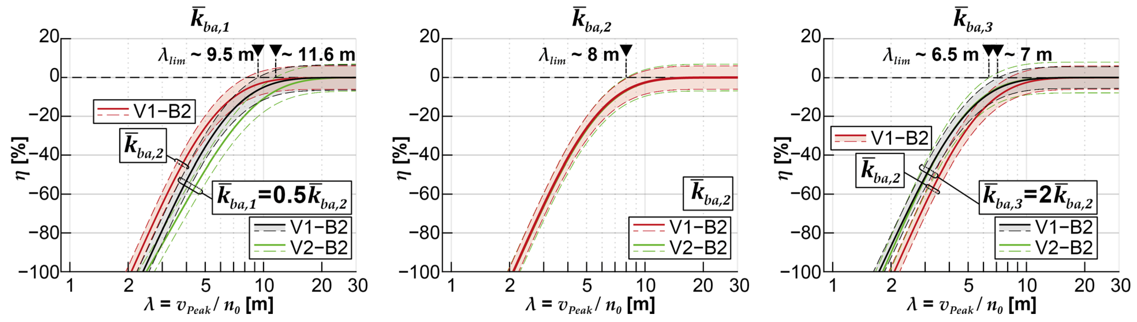
• The influence of the coupling beam model (V1-B2) on the maximum acceleration peaks of the reference model (V1-B1) exhibits a clear dependence on the normalized crossing speed $\lambda =v/n_0$ at which it occurs (see Figure 17). Larger reductions in acceleration can be expected as the normalized speeds decrease. This relationship can be accurately described by an exponential (weighted) regression function, which has a high predictive probability. The reduction in acceleration peaks approaches zero at a normalized speed of approximately 13.2 m. At higher normalized speeds, the results tend to scatter significantly; in some cases, even an increase in acceleration peaks can occur. The upper 95% confidence limit for predicting new observations can be considered reliable within a range of normalized speeds from 2.5 to 8 m. With medium coupling stiffness, the reference model’s calculated acceleration results can be reduced within this range from 0% to −77%.
• In contrast to the coupling beam model (V1-B2), the sole application of the vehicle model DIM (V2-B1) does not exhibit a clear dependence between the percentage reduction in the maximum acceleration peaks and the normalized train speed at which they occur (see Figure 18). Therefore, a regression function of the same form cannot be provided. However, it can be observed that low mass distributions and large ratios of span to structural damping tend to favor a stronger influence of the DIM. In general, as the mass occupancy decreases, the magnitude of acceleration reduction increases. In the maximum case, the reduction can reach up to −75%.
• The comparison between the acceleration reduction achieved by using the coupling beam model and the DIM (V2-B2) versus applying the DIM alone (V2-B1) shows similar results to the comparison with the MLM for the vehicle (see Figure 17 and Figure 19). This indicates that the beneficial impact of the coupling beam model is mainly independent of the specific vehicle model used. In other words, regardless of whether the multi-body model or the MLM is employed, including the coupling beam model consistently leads to favorable acceleration reductions.
• The achievable acceleration reductions strongly depend on the ballast bed stiffness ${\overline{k}}_{ba}$ of the coupling beam model (V1-B2 and V2-B2, see Figure 20, Figure 21 and Figure 22). Lower coupling stiffnesses are associated with more significant reductions in the acceleration peaks of V1-B1. It is worth noting that the regression functions determined for the different vehicle models, DIM (V2-B2) and MLM (V1-B2), may exhibit some deviation, particularly in the case of the lowest coupling stiffness ${\overline{k}}_{ba,1}$.
• The variation in the ballast bed damping coefficient ${\overline{c}}_{ba}$ and structural damping ζ has only marginal effects on the regression functions derived from the results of the entire parameter field, analogously to the exemplary structure (see Figure 22). This observation suggests that a more precise variation in these two parameters may not be necessary for future investigations aiming to describe the influence of coupling beam modeling. It implies that a more generalized approach can be applied, where specific variations in coupling and structural damping can be omitted without significantly compromising the accuracy of the results.

4.4. Limitations of Numerical Study

The numerical study based on the parameter field contains several restrictions, which were made in favor of the computational effort and the reduction to the smallest possible number of variable computational parameters. This is based on the assumption that the influence of the different modeling strategies, particularly the coupling beam modeling, affects the reduction in the accelerations independently of the concrete application and that this influence can best be investigated in isolation by omitting other influencing parameters. Concerning the following aspects, corresponding further investigations are to be carried out in order to confirm the validity of the conclusions drawn from the results for further application areas:

• Bearing Conditions: As mentioned in Section 2.1, only beam-like structures with hinged bearings and no skewness are considered in 2D modeling in the scope of the study presented here. Thus, lateral or torsional vibrations cannot be reproduced. In addition, the bearing conditions, e.g., the vertical flexibility of the bridge bearings, their rotational stiffness, or possible bearing dampers to reproduce the damping capacity resulting from soil–structure interaction, play a significant role regarding the amplitude of calculable structural accelerations and the critical resonance train speeds. However, the mathematical formulation of the equation of motion of the structure used in the investigations presented here does not allow for implementing other support conditions; for this, models discretized based on finite beam elements are better suited.
  Frame structures are of particular importance due to their increased use in the shorter span range. In [55], about 400 bridge structures in the Austrian railway network were investigated, of which about 50% can be classified as single-span beam bridges and 35% as frame structures. The more than 1000 bridges in the Swedish railway network with mainly short spans below 12 m studied in [56] consist of about 43% beam and 48% frame bridges. Due to the usually higher natural frequencies of the frame bridges than beamlike bridges, the influence of the load distribution is expected to have a correspondingly strong effect on the calculated accelerations. The accelerations in the bridge span of a frame bridge can be reproduced by modeling it with rotational restraint of the bridge bearings, e.g., by considering a rotational spring that reproduces the clamping effect. However, implementing a realistic torsional spring stiffness to represent the frame action requires much additional information regarding the structure geometry, the subsoil, and the backfill, whose stiffness significantly affects the restraint action of the bearing walls (see, amongst others, in [57,58,59,60]).
  With the purpose of finding a model as simple as possible and dependent on few parameters, which nevertheless does not exceed the actual structure vibrations in the dimension as the simple reference model, and in favor of a computationally efficient mathematic discretization and programming implementation required for the execution of broad parameter studies, it was renounced to include a more exact implementation of varying support conditions in the study. It is assumed that frame bridges behave like beam bridges of higher natural frequencies and that the influence of the coupling beam modeling affects the respective bridge structure under consideration independently of the bearing conditions. This assumption also needs to be confirmed by further investigations, for example, based on finite bar element modeling.

2.

Track irregularities: The condition of the rails and wheelsets can be taken into account by implementing track irregularities in the loading vectors acting on the train and on the track grid, whereby this is only possible if the train is modeled as a multi-body system, and not if the MLM is used. In the case of poor track conditions, these irregularities can have an unfavorable influence on the results of dynamic calculations, especially on the vehicle accelerations, lateral structural vibrations, and contact forces between rail and wheelsets. On the other hand, studies in [24,37,61,62,63,64,65,66], among others, show that the influence on the vertical structure accelerations is small to negligible, particularly when the irregularities are modeled as a randomized power spectral density function, which could be due to the much higher frequency range in which the vibrations due to track irregularities occur. Nevertheless, this makes applying the coupling beam model in analyses with consideration of track irregularities an interesting research question to be further investigated.

3.

Shear stiffness: The differential equation of the bending line of the Bernoulli–Euler beam used here does not include terms to account for shear stiffness or rotational inertia, as, for example, modeling as a Timoshenko beam would allow. Studies in [3,4,67,68] show that the influence of the rotational inertia on the natural frequency of a Timoshenko beam compared to the Bernoulli–Euler beam is much smaller than that of the shear stiffness. In addition, however, it can also be noted that the influence of both aspects on beams with a span-to-height ratio L/H above 10 generally has only a minor effect on the low-order natural frequencies. Especially for structures with spans below 10 m, the L/H ratio can be lower than 10, which is why for such cases, as well as for structures with high shear compliance (e.g., truss bridges), shear-soft modeling is recommended to obtain realistic vibration results. As with the previously mentioned aspects, the significance of the results obtained from the presented study is yet to be confirmed.

4.5. Final Conclusions and Outlook

The results of the parameter study highlight the significant potential of coupling beam modeling in determining lower computational accelerations compared to a simple beam model. This modeling approach requires only a few input parameters and can be universally applied, independent of the specific train model, presenting a promising complement or alternative to multi-body modeling of the train that considers the vehicle–bridge interaction. This is particularly advantageous in situations where crucial input parameters for multi-body modeling of the train are not accessible, and it tends to have a favorable effect on bridges with different structural parameters.

In the case of the coupling beam model, its impact on the maximum computational accelerations is influenced not only by the normalized train speed, which corresponds to the resonance scenario at which they occur, but also by the applied coupling or ballast bed stiffness. Estimating these characteristic values solely based on the existing literature sources is associated with inadequate certainty, emphasizing the need for a more comprehensive and experimentally underpinned investigation into the dynamic load-bearing behavior of the ballasted track.

When examining the calculation results underlying the regression functions used to describe the impact of coupling beam modeling, it is evident that some positive values are observed, indicating an increase in the maximum calculated acceleration peaks compared to the reference model. This discrepancy can be attributed to simplifications in modeling the coupling beam, such as the linear stiffness assumption of the coupling springs.

The deviation observed in the regression functions describing the influence of the coupling beam for different vehicle models, particularly in the case of the lowest coupling stiffness, warrants more detailed investigation. With such low coupling stiffness, minimal or negligible acceleration peaks may be formed, making a direct comparison with the acceleration peaks of the reference model less feasible and subsequently influencing the resulting regression functions.

However, the overall finding that the vehicle model does not significantly interact with the influence of the coupling beam model in other cases allows for simplifications in future investigations. Extensive analysis of different vehicle models will no longer be necessary to make universally applicable statements regarding the impact of considering track–bridge interaction through a two-layer coupling beam model, significantly reducing the computational effort required for future numerical investigations. The same applies to the limited influence of coupling or ballast bed damping and structural damping as parameters with minimal impact, allowing them to be excluded.

References

1. EN 1990:2002/A1:2005/AC:2010; Eurocode—Basis of Structural Design. CEN European Committee for Standardization: Brussels, Belgium, 2021.
2. Adam, C.; Salcher, P. Dynamic effect of high-speed trains on simple bridge structures. Struct. Eng. Mech. 2014, 51, 581–599. [Google Scholar] [CrossRef]
3. Frýba, L.; Kadecka, S.; ICE Virtual Library. Dynamics of Railway Bridges; Telford, T., Ed.; Publications Sales Department, American Society of Civil Engineers: New York, NY, USA; London, UK, 1996. [Google Scholar]
4. Mähr, T.C. Theoretische und Experimentelle Untersuchungen zum Dynamischen Verhalten von Eisenbahnbrücken mit Schotteroberbau unter Verkehrslast. Ph.D. Thesis, Technische Universtität Wien, Vienna, Austria, 2009. [Google Scholar]
5. Yang, Y.-B.; Yau, J.-D.; Hsu, L.-C. Vibration of simple beams due to trains moving at high speeds. Eng. Struct. 1997, 19, 936–944. [Google Scholar] [CrossRef]
6. Yang, Y.B.; Yau, J.D.; Wu, Y.S. Vehicle-Bridge Interaction Dynamics: With Applications to High-Speed Railways; World Scientific: River Edge, NJ, USA; London, UK, 2004. [Google Scholar]
7. Yang, Y.; Lin, C. Vehicle–bridge interaction dynamics and potential applications. J. Sound Vib. 2005, 284, 205–226. [Google Scholar] [CrossRef]
8. Bruschetini-Ambro, S.-Z.; Fink, J.; Lachinger, S.; Reiterer, M. Ermittlung der Dynamischen Kennwerte von Eisenbahnbrücken unter Anwendung von Unterschiedlichen Schwingungsanregungsmethoden. Bauingenieur 2017, 92, S2–S13. [Google Scholar]
9. Reiterer, M.; Bruschetini-Ambro, S.-Z. Dynamik von Eisenbahnbrücken: Diskrepanz zwischen Messung und Berechnung. Bauingenieur 2019, 94, 9–21. [Google Scholar] [CrossRef]
10. Vospernig, M.; Reiterer, M. Evaluierung der dynamischen Systemeigenschaften von einfeldrigen Stahlbeton-Eisenbahnbrücken: Messtechnische Bestimmung der dynamischen Kennwerte für zwei Versuchsbrücken im gerissenen und ungerissenen Zustand bei unterschiedlichen Ausbauzuständen. Beton-Und Stahlbetonbau 2020, 115, 424–437. [Google Scholar] [CrossRef]
11. Martínez, E.; de Ulzurrun Casals, G.S.-D.; Zanuy, C. Influence of track typology on the dynamic response of short-span high-speed railway bridges. Hormigón y Acero 2023, in press. [Google Scholar]
12. Bonopera, M.; Chang, K.; Chen, C.; Sung, Y.; Tullini, N. Experimental study on the fundamental frequency of prestressed concrete bridge beams with parabolic unbonded tendons. J. Sound Vib. 2019, 455, 150–160. [Google Scholar] [CrossRef]
13. Noble, D.; Nogal, M.; O׳Connor, A.; Pakrashi, V. The effect of prestress force magnitude and eccentricity on the natural bending frequencies of uncracked prestressed concrete beams. J. Sound Vib. 2016, 365, 22–44. [Google Scholar] [CrossRef]
14. Chordà-Monsonís, J.; Romero, A.; Moliner, E.; Galvín, P.; Rodrigo, M. Ballast shear effects on the dynamic response of railway bridges. Eng. Struct. 2022, 272, 114957. [Google Scholar] [CrossRef]
15. Stollwitzer, A.; Bettinelli, L.; Fink, J. The longitudinal track-bridge interaction of ballasted track in railway bridges: Experimental determination of dynamic stiffness and damping characteristics. Eng. Struct. 2023, 274, 115115. [Google Scholar] [CrossRef]
16. Stollwitzer, A.; Fink, J. Mathematical calculation of the damping value of steel railway bridges—Part I: Theoretical background (in German). Stahlbau 2021, 90, 305–315. [Google Scholar] [CrossRef]
17. Stollwitzer, A.; Fink, J. Mathematical calculation of the damping value of steel railway bridges—Part II: Verification on the basis of existing bridges. Stahlbau 2021, 90, 449–462. (In German) [Google Scholar] [CrossRef]
18. Arvidsson, T.; Karoumi, R.; Pacoste, C. Statistical screening of modelling alternatives in train–bridge interaction systems. Eng. Struct. 2014, 59, 693–701. [Google Scholar] [CrossRef]
19. Domenech, A.; Museros, P. Influence of the vehicle model on the response of high-speed railway bridges at resonance. Analysis of the Additional Damping Method prescribed by Eurocode 1. In Proceedings of the 8th International Conference on Structural Dynamics, Eurodyn 2011, Leuven, Belgium, 4–6 July 2011; pp. 1273–1280. [Google Scholar]
20. Doménech, A.; Museros, P.; Rodrigo, M. Influence of the vehicle model on the prediction of the maximum bending response of simply-supported bridges under high-speed railway traffic. Eng. Struct. 2014, 72, 123–139. [Google Scholar] [CrossRef]
21. Glatz, B.; Fink, J. Influence of the calculation models on the dynamic response of 75 steel, composite and concrete bridges. Stahlbau 2019, 88, 470–477. (In German) [Google Scholar] [CrossRef]
22. Glatz, B.; Fink, J. A redesigned approach to the additional damping method in the dynamic analysis of simply supported railway bridges. Eng. Struct. 2021, 241, 112415. (In German) [Google Scholar] [CrossRef]
23. Liu, K.; De Roeck, G.; Lombaert, G. The effect of dynamic train–bridge interaction on the bridge response during a train passage. J. Sound Vib. 2009, 325, 240–251. [Google Scholar] [CrossRef]
24. Cantero, D.; Arvidsson, T.; OBrien, E.; Karoumi, R. Train–track–bridge modelling and review of parameters. Struct. Infrastruct. Eng. 2016, 12, 1051–1064. [Google Scholar] [CrossRef]
25. European Rail Research Institute. ERRI D 214/RP9, Rail Bridges for Speeds >200 km/h; Final Report Part A: Synthesis of the Results of D 214 Research. Part B: Proposed UIC Leaflet; European Rail Research Institute: Utrecht, The Netherlands, 1999. [Google Scholar]
26. Rigueiro, C.; Rebelo, C.; da Silva, L.S. Influence of ballast models in the dynamic response of railway viaducts. J. Sound Vib. 2010, 329, 3030–3040. [Google Scholar] [CrossRef]
27. Stollwitzer, A.; Fink, J. Damping parameters of ballasted track on railway bridges—Part I: Vertical relative displacements in the ballast. Bautechnik 2021, 98, 465–474. (In German) [Google Scholar]
28. Stollwitzer, A.; Fink, J. Damping parameters of ballasted track on railway bridges—Part II: Energy dissipation in the ballasted track and related calculation model (in German). Bautechnik 2021, 98, 552–562. (In German) [Google Scholar]
29. Andersson, C.; Oscarsson, J. Dynamic Train/Track Interaction Including State–Dependent Track Properties and Flexible Vehicle Components. Veh. Syst. Dyn. 1999, 33, 47–58. [Google Scholar] [CrossRef]
30. Kouroussis, G.; Verlinden, O.; Conti, C. Influence of some vehicle and track parameters on the environmental vibrations induced by railway traffic. Veh. Syst. Dyn. 2012, 50, 619–639. [Google Scholar] [CrossRef]
31. Kouroussis, G.; Verlinden, O. Prediction of railway induced ground vibration through multibody and finite element modelling. Mech. Sci. 2013, 4, 167–183. [Google Scholar] [CrossRef]
32. Lei, X.; Zhang, B. The Influence of Track Stiffness Distribution on Dynamic Behavior of Track Transition. ASME/IEEE Jt. Rail Conf. 2011, 54594, 173–180. [Google Scholar] [CrossRef]
33. Lombaert, G.; Degrande, G.; Kogut, J.; François, S. The experimental validation of a numerical model for the prediction of railway induced vibrations. J. Sound Vib. 2006, 297, 512–535. [Google Scholar] [CrossRef]
34. Lou, P.; Yu, Z.W.; Au, F.T.K. Rail-bridge coupling element of unequal lengths for analysing train-track-bridge interaction systems. Appl. Math. Model. 2012, 36, 1395–1414. [Google Scholar]
35. Lou, P. Finite element analysis for train–track–bridge interaction system. Arch. Appl. Mech. 2007, 77, 707–728. [Google Scholar]
36. Moliner, E.; Martínez-Rodrigo, M.D.; Galvín, P.; Monsonís, J.C.; Romero, A. On the vertical coupling effect of ballasted tracks in multi–span simply–supported railway bridges under operating conditions. Struct. Infrastruct. Eng. 2022, 1–23. [Google Scholar] [CrossRef]
37. Nguyen, K.; Goicolea, J.; Galbadón, F. Comparison of dynamic effects of high-speed traffic load on ballasted track using a simplified two-dimensional and full three-dimensional model. Proc. Inst. Mech. Eng. Part F J. Rail Rapid Transit 2014, 228, 128–142. [Google Scholar] [CrossRef]
38. Saramago, G.; Montenegro, P.A.; Ribeiro, D.; Silva, A.; Santos, S.; Calçada, R. Experimental Validation of a Double-Deck Track-Bridge System under Railway Traffic. Sustainability 2022, 14, 5794. [Google Scholar] [CrossRef]
39. Young, T.; Li, C. Vertical Vibration Analysis of Vehicle/Imperfect Track Systems. Veh. Syst. Dyn. 2003, 40, 329–349. [Google Scholar] [CrossRef]
40. EN 1991-2:2003/AC:2010; Eurocode 1: Actions on Structures—Part 2: Traffic Loads on Bridges. CEN European Committee for Standardization: Brussels, Belgium, 2010.
41. prEN 1991-2:2021; Eurocode 1: Actions on Structures—Part 2: Traffic Loads on Bridges and other Civil Engineering Works. CEN European Committee for Standardization: Brussels, Belgium, 2021.
42. RW 08.01.04Dynamische Berechnung von Eisenbahnbrücken, Anhang 1: Zugdefinitionen; ÖBB-Infrastruktur AG: Vienna, Austria, 2022.
43. Petersen, C.; Werkle, H. Dynamik der Baukonstruktionen, 2nd ed.; Springer Vieweg Wiesbaden: Wiesbaden, Germany, 2017. [Google Scholar]
44. Museros, P.; Alarcón, E. Influence of the Second Bending Mode on the Response of High-Speed Bridges at Resonance. J. Struct. Eng. 2005, 131, 405–415. [Google Scholar] [CrossRef]
45. Yang, Y.-B.; Yau, J.-D. Vehicle-Bridge Interaction Element for Dynamic Analysis. J. Struct. Eng. 1997, 123, 1512–1518. [Google Scholar] [CrossRef]
46. Weber, W. Computationally Efficient Simulation Program for the Dynamic Analysis of Railway Bridges using Multi-Body Models and Trigonometric Shape Functions. Diploma Thesis, Technische Universtität Wien, Vienna, Austria, 2009. (In German). [Google Scholar]
47. The Mathworks Inc. MATLAB 2022; The Mathworks Inc.: Natick, MA, USA, 2022. [Google Scholar]
48. Shampine, L.F.; Reichelt, M.W. The MATLAB ODE Suite. SIAM J. Sci. Comput. 1997, 18, 1–22. [Google Scholar] [CrossRef]
49. European Rail Research Institute. ERRI D 214/RP3, Rail Bridges for Speeds >200 km/h; Recommendations for Calculating Damping in Rail Bridge Decks; European Rail Research Institute: Utrecht, The Netherlands, 1999. [Google Scholar]
50. European Rail Research Institute. ERRI D 214/RP8, Rail Bridges for Speeds >200 km/h; Confirmation of Values Against Experimental Data. Part A: Rig Tests to Investigate Ballast Behaviour on Bridges due to High Acceleration Levels Confirmation of the Acceleration Limit for the Ballast. Part B: Comparison of Calculations and Measurements usi; European Rail Research Institute: Utrecht, The Netherlands, 1999. [Google Scholar]
51. Rauert, T.; Bigelow, H.; Hoffmeister, B.; Feldmann, M.; Patz, R.; Lippert, P. On the influence of constructional elements on the dynamic behaviour of filler beam railway bridges (in German). Bautechnik 2010, 87, 665–672. [Google Scholar] [CrossRef]
52. Glatz, B.; Bettinelli, L.; Fink, J. Power cars and vehicle-bridge-interaction in the dynamic calculation of railway bridges (in German). Bautechnik 2020, 97, 453–461. [Google Scholar] [CrossRef]
53. Kotz, S.; Balakrishnan, N.; Johnson, N.L. Continuous Multivariate Distributions, Volume 1: Models and Applications; John Wiley & Sons: New York, NY, USA, 2004; Volume 1. [Google Scholar]
54. Bruckmoser, B. Investigation of the Load-Distributing Effect of the Ballast Bed in Simulations of Railway Bridge Vibrations (in German). Diploma Thesis, Technische Universtität Wien, Vienna, Austria, 2009.
55. Unterweger, H.; Taras, A.; Schörghofer, A. Bestandsbrücken im Hochgeschwindigkeitsnetz-Vorgehensweise und Auswahl Maßgebender Brücken bei Einfeldtragwerken; Graz University of Technology: Graz, Austria, 2015. [Google Scholar]
56. Johansson, C.; Nualláin, N.; Pacoste, C.; Andersson, A. A methodology for the preliminary assessment of existing railway bridges for high-speed traffic. Eng. Struct. 2014, 58, 25–35. [Google Scholar] [CrossRef]
57. Heiland, T.; Aji, H.D.; Wuttke, F.; Stempniewski, L.; Stark, A. Influence of soil-structure interaction on the dynamic characteristics of railroad frame bridges. Soil Dyn. Earthq. Eng. 2023, 167, 107800. [Google Scholar] [CrossRef]
58. Ülker-Kaustell, M.; Karoumi, R.; Pacoste, C. Simplified analysis of the dynamic soil–structure interaction of a portal frame railway bridge. Eng. Struct. 2010, 32, 3692–3698. [Google Scholar] [CrossRef]
59. Zangeneh, A. Dynamic Soil-Structure Interaction Analysis of Railway Bridges: Numerical and Experimental Results. Licenciate Thesis, KTH Royal Institute of Technology, Stockholm, Sweden, 2018. [Google Scholar]
60. Zangeneh, A. Dynamic Soil-Structure Interaction Analysis of High-Speed Railway Bridges: Efficient Modeling Techniques and Experimental Testing. Ph.D. Thesis, KTH Royal Institute of Technology, Stockholm, Sweden, 2021. [Google Scholar]
61. Dinh, V.N.; Du Kim, K.; Warnitchai, P. Dynamic analysis of three-dimensional bridge–high-speed train interactions using a wheel–rail contact model. Eng. Struct. 2009, 31, 3090–3106. [Google Scholar] [CrossRef]
62. Lei, X.; Noda, N.A. Analyses of dynamic response of vehicle and track coupling system with random irregularity of track vertical profile. J. Sound Vib. 2002, 258, 147–165. [Google Scholar] [CrossRef]
63. Lou, P.; Zeng, Q.-Y. Formulation of Equations of Motion for a Simply Supported Bridge under a Moving Railway Freight Vehicle. Shock. Vib. 2007, 14, 429–446. [Google Scholar] [CrossRef]
64. Majka, M.; Hartnett, M. Dynamic response of bridges to moving trains: A study on effects of random track irregularities and bridge skewness. Comput. Struct. 2009, 87, 1233–1252. [Google Scholar] [CrossRef]
65. Peixer, M.; Montenegro, P.; Carvalho, H.; Ribeiro, D.; Bittencourt, T.; Calçada, R. Running safety evaluation of a train moving over a high-speed railway viaduct under different track conditions. Eng. Fail. Anal. 2020, 121, 105133. [Google Scholar] [CrossRef]
66. Wu, Y.-S.; Yang, Y.-B.; Yau, J.-D. Three-Dimensional Analysis of Train-Rail-Bridge Interaction Problems. Veh. Syst. Dyn. 2001, 36, 1–35. [Google Scholar] [CrossRef]
67. Huang, T.C. The Effect of Rotatory Inertia and of Shear Deformation on the Frequency and Normal Mode Equations of Uniform Beams With Simple End Conditions. J. Appl. Mech. 1961, 28, 579–584. [Google Scholar] [CrossRef]
68. Timoshenko, S.; Young, D.H.; Weaver, W. Vibration Problems in Engineering, 4th ed.; Wiley: New York, NY, USA, 1974. [Google Scholar]
Figure 1. Possible modeling of the ballasted superstructure on any subsoil (bridge structure or embankment).
Applsci 13 08746 g001
Figure 2. Applied two-dimensional mechanical models: (a) models of the bridge structure; (b) models of the high-speed train.
Applsci 13 08746 g002
Figure 3. Combinations of span and fundamental frequencies of existing concrete, filler beam, steel, and composite bridge structures as the basis for the numerical study.
Applsci 13 08746 g003
Figure 4. Combinations of span and mass distribution of existing concrete, filler beam, steel and composite bridge structures as the basis for the numerical study.
Applsci 13 08746 g004
Figure 5. Literature values of stiffness and damping coefficients of the ballast superstructure according to two- to four-layer models, modified from [28].
Applsci 13 08746 g005
Figure 6. Probability of structural parameter combination based on multivariate regression and a catalog of existing bridges.
Applsci 13 08746 g006
Figure 7. Acceleration results for one exemplary structure and four different modeling alternatives.
Applsci 13 08746 g007
Figure 8. Acceleration results for one exemplary structure, four different modeling alternatives, and variation in structural damping ζ.
Applsci 13 08746 g008
Figure 9. Acceleration results for one exemplary structure, four different modeling alternatives, and variation in ballast bed stiffness k ¯ b a .
Applsci 13 08746 g009
Figure 10. Acceleration results for a parameter field of bridges for 100 km/h ≤ v ≤ 420 km/h and V1-B1.
Applsci 13 08746 g010
Figure 11. Train speeds with max > 3.5 m/s2, evaluated for a parameter field of bridges and V1-B1.
Applsci 13 08746 g011
Figure 12. Train speeds with max > 3.5 m/s2, evaluated for a parameter field of bridges and V2-B1.
Applsci 13 08746 g012
Figure 13. Train speeds with max > 3.5 m/s2, evaluated for a parameter field of bridges and V1-B2 ( k ¯ b a , 2 , c ¯ b a , 2 ).
Applsci 13 08746 g013
Figure 14. Train speeds with max > 3.5 m/s2, evaluated for a parameter field of bridges and V2-B2 ( k ¯ b a , 2 , c ¯ b a , 2 ).
Applsci 13 08746 g014
Figure 15. Proportion of bridge structures with max > 3.5 m/s2 at specific train speed intervals depending on a dynamic calculation model, evaluated for concrete and filler beam structures (left) and steel and composite structures (right).
Applsci 13 08746 g015
Figure 16. Statistical evaluation of critical train speed vlim (max > 3.5 m/s2) depending on a dynamic calculation model and mass distribution μ.
Applsci 13 08746 g016
Figure 17. Evaluation of influence η of V1-B2 on acceleration peaks, compared to V1-B1, distinguished by mass distribution.
Applsci 13 08746 g017
Figure 18. Evaluation of influence η of V2-B1 on acceleration peaks, compared to V1-B1, distinguished by mass distribution.
Applsci 13 08746 g018
Figure 19. Evaluation of influence η of V2-B2 on acceleration peaks, compared to V2-B1, distinguished by mass distribution.
Applsci 13 08746 g019
Figure 20. Comprehensive depiction of regression functions η(λ) for V1-B1 and V2-B2.
Applsci 13 08746 g020
Figure 21. Comparison of regression functions η(λ) for different coupling stiffnesses k ¯ b a .
Applsci 13 08746 g021
Figure 22. Comparison of regression functions η(λ) for different coupling stiffnesses k ¯ b a (left), damping coefficients c ¯ b a (center), and structural dampings ζ.
Applsci 13 08746 g022