Article

Identical Parallel Machine Scheduling Considering Workload Smoothness Index

1
Glorious Sun School of Business and Management, Donghua University, Shanghai 200051, China
2
School of Economics and Management, Tongji University, Shanghai 200092, China
*
Author to whom correspondence should be addressed.
Appl. Sci. 2023, 13(15), 8720; https://doi.org/10.3390/app13158720
Submission received: 3 July 2023 / Revised: 25 July 2023 / Accepted: 26 July 2023 / Published: 28 July 2023
(This article belongs to the Special Issue Advanced Manufacturing Technologies and Their Applications, Volume II)

Abstract

:
Workload balance is significant in the manufacturing industry. However, on the one hand, some existing specific criteria cannot achieve the minimization workload imbalance of parallel machines. On the other hand, there are few algorithms in existing studies that can effectively solve the parallel machine scheduling problem with the objective of minimizing workload imbalance. Inspired by this, we investigate an identical parallel machine scheduling problem with the objective of the minimum workload smoothness index. We first establish a mathematical model for the considered problem and then linearize its objective function. We prove the NP-hardness of the problem by reducing the PARTITION problem to it, and we provide both the upper bound and lower bound of the studied problem. An efficient genetic algorithm and an improved list scheduling algorithm are also proposed to efficiently address the considered problem. The numerical results demonstrate the effectiveness of the proposed methods.

1. Introduction

Parallel machine scheduling systems have been extensively applied in various production and manufacturing industries [1]. In parallel machine scheduling, it generally contains two decision issues, i.e., sequencing and job assignment [2,3]. Various optimization objectives, including the makespan and the total completion time, have been well addressed in previous studies [4,5,6,7]. In addition to the above classical objectives, workload balance between the machines together with the corresponding operators is also a major aspect of decision making in manufacturing industry [8,9,10]. It contributes to reducing the idleness and work-in-process and removing bottlenecks [8,11]. Minimum imbalance is actually beneficial for minimizing the inventory of finished goods [12].
The solutions with the classical minimum objective of the makespan or the total completion time may induce the workload balance between the parallel machines to a large extent. However, the above solutions cannot guarantee their optimality when we aim to minimize the imbalance of workloads between the machines. Therefore, some previous works have investigated other specific criteria to measure the workload imbalance, such as the Average Relative Percentage of Imbalance ( A R P I ) [12], Total Imbalance ( T B ) [13] and even Total Workload [14].
In this work, we introduce the workload smoothness index ( S I ) to the identical parallel machine scheduling problem. The index of S I was introduced by Moodie and Young [15] to measure the balance level of workloads between the neighboring workstations in an assembly line environment. To our best knowledge, this is the first study to introduce S I as an optimization objective into parallel machine scheduling problems. We observe that S I may generate a better solution in terms of the workload balance between the parallel machines, comparing with A R P I , T B and some other measurements. We first present the formulae of the above indices and then give two examples to illustrate their performance difference. The indices are given by S I = i M ( W max W i ) 2 , A R P I = 1 m · ( i M W max W i W max ) and T B = i M | i M W i m W i | , where W max is the maximum workload or the makespan, W i is the workload of machine i, and M is the set of machines. In Example 1, there are f i v e jobs J 1 , J 2 , J 3 , J 4 , J 5 to be processed on f o u r parallel machines. The corresponding processing times of the jobs are 1, 2, 3, 6 and 8, respectively. For both problems P m | | C max and P m | | A R P I , all the three solutions shown in Figure 1a–c are optimal with the minimum objective value of C max = W max = 8 and A R P I = 1 4 · ( i = 1 4 8 W i 8 ) = 3 / 8 , respectively. For problem P m | | T B , however, only the two solutions in Figure 1b,c are optimal with the minimum objective value of T B = i = 1 4 | i M W i 4 W i | = 8 . For the considered problem P m | | S I in this work, we observe that only solution Figure 1b is optimal with the corresponding objective value of S I = i = 1 4 ( 8 W i ) 2 = 54 , while the other two solutions in Figure 1a,c are of the objective values of S I = 74 and S I = 62 , respectively. That is, the job assignment in Figure 1b has the best workload balance among the three solutions.
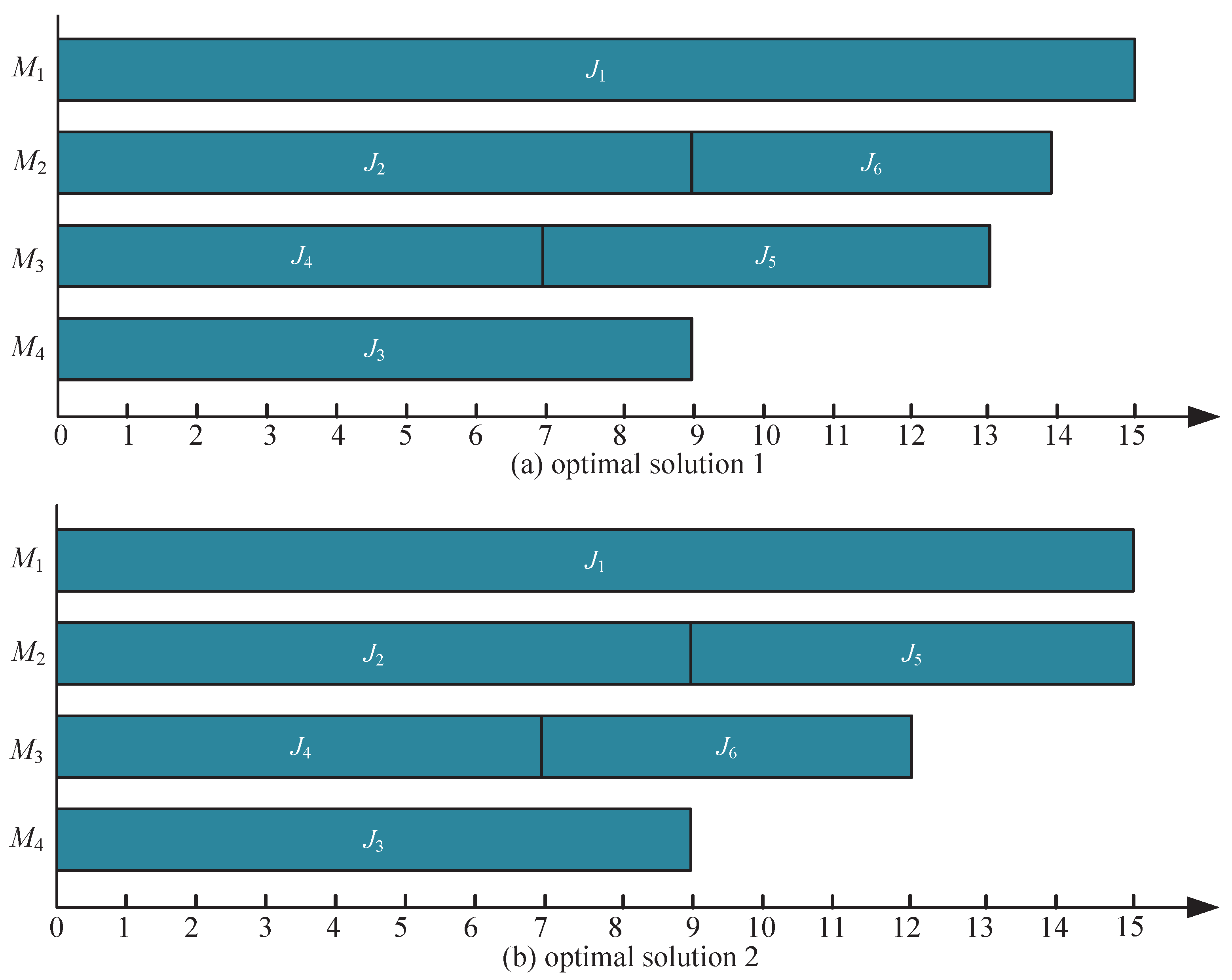
In the above example, we find that the solution in Figure 1b is also the only optimal schedule for problem P m | | M W D where M W D = max i M W max W i W max . The following Example 2, however, reveals that index S I also better guarantees workload balance than M W D . In Example 2, there are s i x jobs with processing times 15, 9, 9, 7, 6, and 5 to be processed on f o u r machines. Figure 2 reports two optimal solutions to problem P m | | M W D , while the solution in Figure 2a outperforms that in Figure 2b for problem P m | | S I . The corresponding values of S I are equal to 41 and 45 , respectively. That is, the solution in Figure 2a has better workload balance than that in Figure 2b.
By the above two examples, we believe that although the smoothness index ( S I ) is currently used in assembly line processing systems in previous studies, it is the most feasible index to measure the workload balance in identical parallel machine scheduling compared with other existing criteria. Motivated by this, we investigate the identical parallel machine scheduling problem with the objective of minimizing the workload smoothness index, i.e., the P m | | S I problem. The main contributions of this study are as follows.
(1)
We introduce smoothness index to identical parallel machine scheduling and prove the NP-hardness of the considered problem.
(2)
A mathematical model with a minimizing smoothness index is established, and both upper and lower bounds are provided.
(3)
To quickly find high-quality feasible solutions, an efficient genetic algorithm and an improved list scheduling algorithm are proposed. Numerical experiments show that the proposed genetic algorithm can output high-quality feasible solutions for small-scale instances. For large-scale instances, the proposed improved list scheduling algorithm outperforms the list scheduling algorithm based on LPT, SPT, and RPT rules. Please refer to Section 6 for specific details.
The remainder of this paper is organized as follows. Section 2 reviews previous studies on the parallel machine workload balancing problem and smoothness index in the assembly line environment. Section 3 builds a mathematical model for the considered problem and linearizes its objective function. We prove the NP-hardness of the P m | | S I problem and present both upper and lower bounds in Section 4. Section 5 proposes a genetic algorithm and an improved list scheduling algorithm to solve the considered problem. We also conduct numerical experiments to evaluate the performance of proposed heuristic algorithms in Section 6. Finally, Section 7 concludes this work.

2. Literature Review

Many previous studies have paid attention to the issue of workload balance in parallel machine scheduling, and various measures other than S I have been adopted to evaluate the qualities of solutions. On the other hand, researchers have also adopted the index of S I to evaluate solution qualities in the assembly line balancing problem. In the following, we review the related literature in two aspects: the parallel machine workload balancing problem and smoothness index in the assembly line environment.

2.1. Parallel Machine Workload Balancing Problem

For the parallel machine workload balancing problem, Rajakumar et al. [11] introduce the index of total relative percentage of workload imbalances, i.e., R P I = i M W max W i W max · 100 % , where W i is the workload of machine i, and W max = max { W 1 , W 2 , W i , , W m } . They propose three list scheduling algorithms based on the following rules: Random, SPT (shortest processing time first), and LPT (longest processing time first). Experimental results show that the list scheduling algorithm based on the LPT rule outperforms the other two algorithms. Moon et al. [13] study the workload balancing problem in a semi-automatic parallel machine shop in which two types of machines are operated by several operators. The objective is to minimize the imbalance of the workloads among the operators, i.e., to minimize T B = i M | i M W i m W i | . Ouazene et al. [16] investigate the parallel machine workload balancing problem with the objective of minimizing the maximum workload difference between machines, i.e., minimizing M W D = max i M W max W i W max .
Yildirim et al. [17] study the parallel machine workload balancing problem with sequence-dependent setup times and define the maximum allowable level α of imbalance. That is, the sum of the processing times and setup times of jobs assigned to machine i, denoted by W i , has to be within some tolerance. More precisely, W i 1 m · W t o t a l ( 1 + α ) and W i 1 m · W t o t a l ( 1 α ) , where W t o t a l is sum of the total processing time and the total setup time of all the jobs. Keskinturk et al. [12] also address the parallel problem scheduling problem with sequence-dependent setup times, in which the objective is to minimize the average relative percentage of imbalance ( A R P I ), i.e., to minimize A R P I = 1 m · ( i M W max W i W max ) × 100 % .
Ho et al. [18] introduce a criterion named the normalized sum of squared workload deviations (NSSWD) to minimize the workload imbalance. They prove that an NSSWD-optimal schedule is necessarily a makespan-optimal one. Walter and Lawrinenko [19] explain such a proof is incorrect under the case of m 3 . For solving the problem under the case of m 3 , Schwerdfeger and Walter [20] propose an algorithm based on a local search procedure. Theoretically, an NSSWD-optimal schedule is necessarily an SI-optimal one. However, relatively few studies apply NSWWD to achieve the workload imbalance minimization. Consequently, the linearization process of NSSWD is relatively unexplored, which makes the problem difficult to be directly solved by calling commercial solvers. Moreover, few studies on problem P m | | N S S W D consider the given maximum workload constraint of machines. Besides, some works consider controllable processing in order to achieve balanced workloads (i.e., smooth processes) on (neighbor) machines [21,22].
In the above studies, various indices have been proposed to deal with the parallel machine workload balancing problem. As shown in Example 1 and Example 2, however, the indices may not guarantee a solution with the best possible balance between the parallel machines. Therefore, we adopt the smoothness index rather than any of the above indices as the optimization objective of the considered problem in this study.

2.2. Smoothness Index in the Assembly Line Environment

Moodie and Young [15] are the first to introduce the smoothness index in the assembly line balancing problem, i.e., S I = i M ( W max W i ) 2 , where W max is the given cycle time constraint of the assembly line. Kim et al. [23] further present a new heuristic procedure based on the genetic algorithm for the assembly line balancing problem with the objective of maximizing the workload smoothness index. Scholl [24] use S I to measure the balance level of the working time between the workstations of the assembly line. Emde et al. [25] investigate several objectives to smoothen the workload, and the proposed measures are systematically tested in a comprehensive computational study. Testing results suggest that workload smoothing is an essential task in mixed-model assembly lines. Nearchou [26] proposes a novel method based on PSO to address a simple assembly line balancing problem (SALBP), minimizing the cycle time and the workload smoothing. Azizoǧlu and İmat [27] consider the SALBP problem with a fixed number of workstations and prespecified cycle time. For the objective of minimizing the value of S I , they develop several optimality properties and bounding mechanisms and then propose an efficient branch-and-bound algorithm. Finco et al. [28] study an assembly line balancing problem where the factor of human energy consumption is included and the objective is to minimize the value of S I . They propose several solution methodologies and make comparison of their performance via computational experiments.
As shown above, the smoothness index S I has been well studied in the assembly line balancing problem. In this work, we adopt the smoothness index to evaluate the level of workload balance between the identical parallel machines in order to provide a most reasonable job scheduling solution in manufacturing decision making, considering the fairness of the workload.

3. Problem Statement and Mathematical Model

3.1. Problem Statement

There are n jobs with positive processing times p 1 , p 2 , , p n to be processed on m identical parallel machines. All the jobs are released at time 0, and the objective is to minimize the workload smoothness index, i.e., minimizing S I = i M ( W max W i ) 2 , where W max is the maximum workload of the machine and W i is the workload of machine i. The value of W i is exactly the total processing time of the jobs assigned to machine i in any processing schedule. Adopting the classical three-notation method, we denote the considered problem as P m | | S I .
The problem under consideration is based on the following fundamental assumptions.
(1)
Each machine can only process one job at a time;
(2)
The setup time of processing any job on each machine is negligible;
(3)
All the machines are available for processing jobs from time 0.
Below, we first present basic parameters and decision variables and then establish one mathematical model for problem P m | | S I . We further linearize the objective function and thus provide an equivalent linear programming model.

3.1.1. Input Parameters

M
: set of machines indexed by i, i.e., i M = { 1 , 2 , , m } ;
J
: set of jobs indexed by j, i.e., j J = { 1 , 2 , , n } ;
p j
: the processing time of job j J ;
W max
: the given maximum workload limitation of machines.

3.1.2. Decision Variables

x i j
: a binary variable equal to 1 if job j J is processed on machine i M and 0 otherwise;
y i j j
: a binary variable equal to 1 if jobs j J and j J { j } are processed on machine i M and 0 otherwise;
W i
: the workload of machine i M .

3.2. Mathematical Model

The objective is to minimize the S I , as shown in Formula (1).
[ P 1 ] : min S I = i M ( W max W i ) 2 .
subject to
i M x i j = 1 , j J
W i = j J x i j · p j , i M
W i W max , i M
x i j { 0 , 1 } , i M , j J
W i S + , i M
Constraint (2) guarantees that each job can only be processed in a machine. Constraint (3) calculates the workload of machine i M . Constraint (4) ensures that the workload of each machine cannot exceed the maximum workload constraint. Constraints (5) and (6) give the ranges of the variables, where S + is the set of positive real numbers.

3.3. Objective Function Linearization

In model [P1], the objective function is non-linear. To transform the model into a linear programming and then solve it via CPLEX or other commercial solvers, we linearize the objective function in this subsection.
Theorem 1.
For problem P m | | S I , minimizing S I is equivalent to minimizing
i M j J j J { j } p j · p j · y i j j
Proof. 
Azizoǧlu and İmat [27] have proved that minimizing S I 2 is equivalent to minimizing
i M ( j J p j 2 · y i j j + 2 · j J j J { j } p j · p j · y i j j )
Furthermore, since i M y i j j = i M x i j = 1 , i M ( j J p j 2 · y i j j ) is a constant. Therefore, minimizing S I is equivalent to minimizing Equation (8). The proof is completed.    □
According to Theorem 1, mathematical model [P1] can be reformulated as below
[ P 2 ] : min f = i M j J j J { j } p j · p j · y i j j
subject to Constraints (2)–(6) and the following Constraints (9)–(11).
y i j j x i j + x i j 1 , i M , j J , j J { j }
y i j j x i j , i M , j J , j J { j }
y i j j { 0 , 1 } , i M , j J , j J { j }
Constraints (9) and (10) give the processing sequence of jobs on each machine. Constraint (11) gives the range of the variables. Since [P2] is a linear programming model, we can directly adopt some commercial solver such as CPLEX to solve it.

4. Theoretical Analysis

4.1. NP-Hardness

For problem P m | | S I , we prove its NP-hardness via reduction from the PARTITION problem.
Theorem 2.
Problem P m | | S I is NP-hard.
Proof. 
We prove the theorem by reducing PARTITION to the considered problem. We first phrase the classical PARTITION problem below.
PARTITION: Given n positive real numbers S = { a 1 , a 2 , a n } with k = 1 2 j = 1 n a j , do there exist two disjoint subsets S 1 , S 2 such that S 1 S 2 = S and j S 1 a j = j S 2 a j = k ?
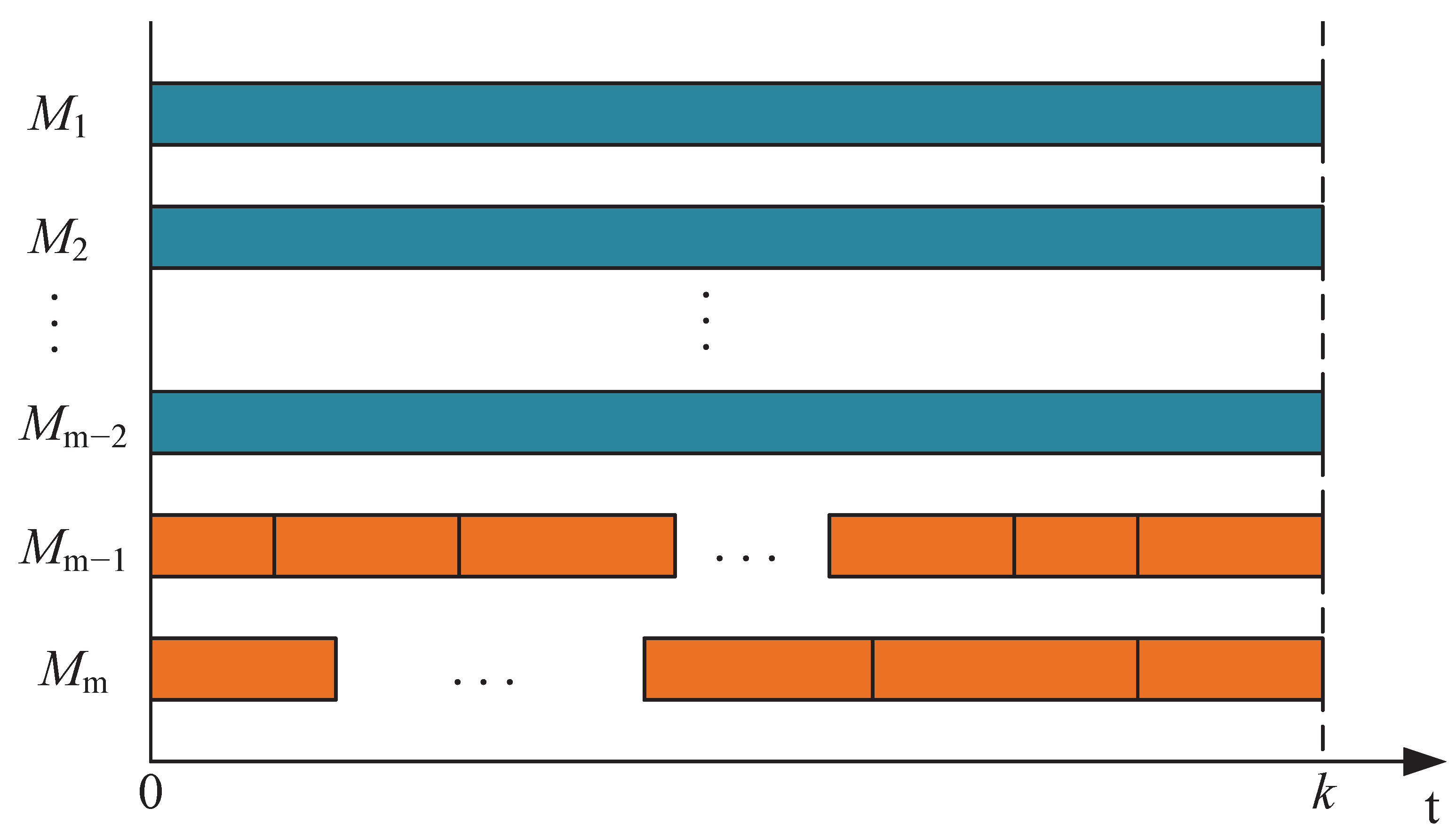
For problem P m | | S I , we construct a job input instance with n + m 2 jobs that are to be processed on m ( 2 m n ) machines. Let p j = a j for 1 j n , and p j = k for n + 1 j n + m 2 . Hence, 1 j n p j = 2 · k and 1 j n + m 2 p j = m · k . We claim that if there exists a YES answer to the PARTITION problem, implying the existence of two disjoint sets S 1 , S 2 with j S 1 a j = j S 2 a j = k , then there is an optimal solution to problem P m | | S I , in which the first n jobs are partitioned into two job sets with the same total processing time equal to k and assigned to two machines with the same workload of k. For the remaining m 2 jobs, each of them is assigned to one of the remaining machines. As shown in Figure 3, all the machines are of the same workload of k and S I = 0 in the optimal solution.
On the other hand, if there exists an optimal solution to problem P m | | S I , then we conclude that the first n jobs must be partitioned into two job sets with the same total processing time. With p j = a j for 1 j n , it indicates the existence of two disjoint subsets S 1 , S 2 with j S 1 a j = j S 2 a j = k . The proof is completed.    □

4.2. Upper and Lower Bounds

Theorem 3.
Assume that job J k ( k [ 1 , m ] ) has the longest processing time among the job set. For any feasible solution of a job input instance, the upper bound of the objective value is as follows.
U B = m · W max 2 + ( j J { k } p j m + p k 2 · W max ) · j J p j .
Proof. 
In the optimal solution, we have W i j J { k } p j m + p k and i M W i = j J p j . Thus, we can know that
S I 2 = i M ( W max W i ) 2 = m · W max 2 2 · i M W max · W i + i M W i 2 = m · W max 2 + i M W i · ( W i 2 · W max ) m · W max 2 + ( j J { k } p j m + p k 2 · W max ) · j J p j = U B 2 .
Hence, S I U B . The proof is completed.    □
Theorem 4.
L B = m · ( W max j J p j m ) 2 is a lower bound of problem P m | | S I .
Proof. 
Let Δ i = W i j J p j m . As i M Δ i = 0 ,
S I 2 = i M ( W max j J p j m Δ i ) 2 = i M [ ( W max j J p j m ) 2 + Δ i 2 2 · Δ i · ( W max j J p j m ) ] = i M [ ( W max j J p j m ) 2 + Δ i 2 ] 2 · ( W max j J p j m ) · i M Δ i = i M [ ( W max j J p j m ) 2 + Δ i 2 ] .
Due to i M Δ i 2 0 , S I 2 m · ( W max j J p j m ) 2 = L B 2 . Hence, S I L B . The proof is completed.    □
Lemma 1.
In the optimal solution of problem P m | | S I , the workload imbalance between any two machines is less than or equal to the processing time of the smallest job on the machine with a larger workload.
Proof. 
According to Azizoǧlu and İmat [27], model [P2] and the following model [P3] share the common optimal solution.
[ P 3 ] : min f = i M ( W i ) 2
subject to Constraints (2)–(6).
Let l J , i and i denote the smallest job on the machine with a larger workload, the machine with a larger workload and the machine with a smaller workload. We assume that W j W i p l . We only need to prove the following inequality.
( W i ) 2 + ( W i ) 2 ( W i p l ) 2 + ( W i + p l ) 2
Due to W j W i p l , we have
( W i p l ) 2 + ( W i + p l ) 2 = ( W i ) 2 + ( W i ) 2 + 2 · ( p l ) 2 2 · p l · ( W i W i ) ( W i ) 2 + ( W i ) 2
Therefore, Lemma 1 is proved. The proof is completed.    □
Theorem 5.
If n > m , there is no machine with a workload of 0 in the optimal solution of problem P m | | S I .
Proof. 
According to Lemma 1, it is evident that Theorem 5 holds. Therefore, the proof process is omitted for simplicity.    □

5. Heuristic Algorithms

In this section, we further construct an efficient genetic algorithm and an improved list algorithm to solve the considered problem.

5.1. Genetic Algorithm Based on Bounding Mechanisms

The genetic algorithm simulates the natural selection and genetic mechanism in Darwin’s biological evolution theory. As meta-heuristic search algorithms, genetic algorithms have been extensively used to solve scheduling problems in manufacturing systems [29] and other NP-hard problems [30]. In the genetic algorithm, each chromosome represents a feasible solution [31]. For problem P m | | S I , we propose an improved genetic algorithm based on bounding mechanisms, which is denoted as G A B M .

5.1.1. Chromosome Representation

For each chromosome, the position of a gene represents the index of the job, while the value of the gene represents the index of a machine. For example, in Figure 4, the first gene is 1: that is to say, job J 1 is to be processed on machine 1.

5.1.2. Fitness Function

In the genetic algorithm, the fitness value of a chromosome corresponds to the probability that it is selected as the parent chromosome. We assume that N I N D is the population size, and o b j ( v ) is the corresponding objective value of chromosome v in the population. Since this study aims to minimize the workload smoothness index, we define the fitness value of chromosome v as 1 / o b j ( v ) . For the case where the solution (or a chromosome) is infeasible, we set the corresponding objective value to be a sufficiently large real number, implying that its fitness value is infinitesimal.

5.1.3. Initialization of Chromosomes

In order to reduce the solution space and find the optimal solution more accurately, we generate the initial population by the B M algorithm. The pseudo-code of the algorithm is described in Algorithm 1, where c h r o m ( v , j ) means the jth gene of chromosome v. In the B M algorithm, U B is the upper bound of the optimal solution which can be obtained by Theorem 3, and L B is the lower bound of the optimal solution which can be obtained by Theorem 4. Let ω = j J { k } p j m + p k , where job J k is with the maximum processing time.

5.1.4. Crossover and Mutation

After two parents are selected, we then randomly select two genes from the two parents, respectively, to cross based on two-point crossover. Similarly, after a chromosome is randomly selected in the population, for completing mutation, we randomly select a gene that can guarantee the maximum workload of the chromosome after mutation is smaller or equal to ω to mutate. In addition, after crossover, if the maximum workloads of any two offspring are large than ω , we will copy their parents as offspring.
Algorithm 1  B M algorithm
Require:  U B , L B , N I N D , M , { p 1 , p 2 , , p n }
1:
for  v = 1 : N I N D   do
2:
   for  j = 1 : n  do
3:
      κ = { i | i M & w i + p j ω }
          %Define a machine set κ in which the current workload of all jobs plus p j is less than or equal to ω
4:
      c h r o m ( v , j ) = κ ( σ ) , where σ is a random integer less than the length of set κ
          %A machine is randomly selected in set κ to process job j J
5:
   end for
6:
   Calculate the fitness of chromosome v, i.e., o b j ( v )
7:
   while  o b j ( v ) > U B  do
8:
     Chromosome v is regenerated according to the above rules
          %If the objective value of the corresponding chromosome is larger than the given upper bound, a new chromosome is generated to replace it
9:
     Calculate the fitness of chromosome v
10:
   end while
11:
   if  o b j ( v ) = L B  then
12:
      N I N D chromosomes v are copied as the initial population
          %If the corresponding objective value of the chromosome is equal to the given lower bound, N I N D copies of that chromosome will be used as the initial population
13:
      v N I N D + 1
14:
   end if
15:
end for
16:
return Initial chromosome population

5.2. List Scheduling Algorithms

List scheduling algorithms (LSAs) perform well in solving parallel machine scheduling problems with regard to machine utilization criteria [3,32]. The main idea of LSAs is to assign each job in the list of waiting jobs to the machine with the minimum workload [16]. In practice, there are different strategies for selecting jobs from the waiting job list. We denote the list scheduling algorithm based on the SPT (shortest processing time first), LPT (longest processing time first) and RPT (random processing time) rules by L S A S P T , L S A L P T and L S A R P T , respectively. For convenience, we show the pseudo-code of LSAs in Algorithm 2.
Algorithm 2 List scheduling algorithms (LSAs)
Require:  m , n , { p 1 , p 2 , , p n }
1:
Sequence the jobs in the order of LPT, SPT or random.
2:
for  j = 1 : n   do
3:
   Assign job j J to the machine with the currently minimum workload
4:
   for  i = 1 : m  do
5:
     Calculate the current workload of machine i, that is, the sum of the processing time of the jobs currently assigned to machine i
6:
   end for
7:
end for
8:
return The objective value and the corresponding schedule

5.3. An Improved List Scheduling Algorithm

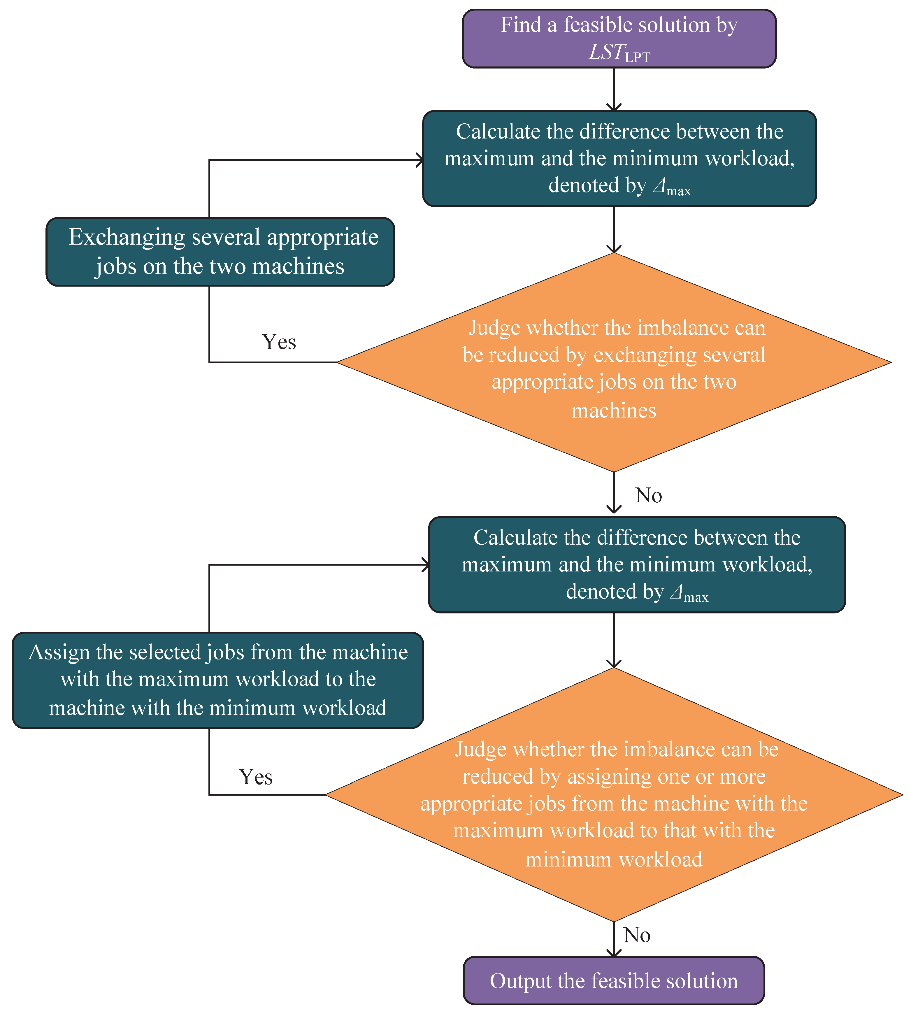
Previous studies show that the list scheduling algorithm based on the LPT rule has better performance in solving workload balancing problems (e.g., [32]). Inspired by Lemma 1, we propose an improved list scheduling algorithm based on the LPT rule, which is denoted by I L S A L P T . The main idea of I L S A L P T algorithm is to minimize the difference between the maximum workload and the minimum workload. A detailed description of the main idea of the I L S A L P T algorithm is shown in Figure 5.
For example, suppose there are seven jobs to be processed on two machines. The corresponding processing times of the jobs are (8, 9, 8, 6, 8, 7, 6). Let the maximum workload constraint be 29. The solution of the L S A L P T algorithm is shown in Figure 6a. The working time of machine 1 is 6 longer than that of machine 2. If we can remove 3 (6/2) units’ processing times from machine 1 to machine 2, the optimal solution can be obtained. However, it is not difficult to find that this method is not feasible for this case. Nevertheless, we can reduce the working time on machine 1 by 3 units as much as possible by exchanging the positions of job J 2 and job J 6 ; the detail is shown in Figure 6b. After the above operations, we can obtain a better feasible solution. To keep our algorithm more understandable, the pseudo-code of the I L S A L P T algorithm is described in Algorithm 3.
Algorithm 3  I L S A L P T algorithm
Require:  m , n , { p 1 , p 2 , , p n }
1:
Find a feasible solution by L S T L P T
2:
Calculate the difference between the maximum workload and the minimum workload, denoted by Δ max
3:
Determine the longest job k which is processed on the machine with the maximum workload
4:
Determine the set, denoted by η , of jobs that are processed on the machine with the minimum workload
5:
α = { j | j η & 0 < p k p j < Δ max } % Find the job j in set η satisfying 0 < p k p j < Δ max
6:
while α ϕ do
7:
   Assign job J k to the machine with the minimum workload
8:
   Seek the job denoted by j in set α whose absolute value of the difference between its processing time and p k is the closest to Δ max / 2 , then assign the job to the machine with the maximum workload
9:
    α = α { j }
10:
   Update set α and Δ max
11:
end while
12:
β = { j | j η & p j < Δ max } % Find the job j processed on the machine with the maximum workload satisfying p j < Δ max
13:
while β ϕ do
14:
   Assign the job denoted by j in set β whose processing time is closest to Δ max / 2 to the machine with the minimum workload
15:
    β = β { j }
16:
   Update set β and Δ max
17:
end while
18:
Calculate the objective value
19:
return The objective value and the feasible solution

6. Numerical Experiments

CPLEX is a common commercial solver for finding exact solutions of linear programming models. Hence, we select the optimal solution obtained by CPLEX solver as the benchmark to evaluate the performance of G A B M , I L S A L P T , L S A S P T , L S A L P T and L S A R P T algorithms in small-scale numerical experiments. Notice that in this work, we first apply CPLEX to solve a mixed-integer linear programming model [P2] to obtain the value of W i ( i M ). Then, the optimal objective value of model [P1] can be obtained by Formula (1). To reveal the performance difference between the above heuristic algorithms, we define a relative error g a p 1 = o b j o b j * o b j * × 100 % in small-scale numerical experiments, where o b j represents the objective value of the solution obtained by the corresponding algorithm. In small-scale instances, g a p 1 measures the relative error between the objective value of each heuristic algorithm and that of CPLEX. In large-scale instances, we define g a p 2 (please refer to the Section 6.2) to measure the relative error between the objective value of each heuristic algorithm and that of L S A L P T . All the numerical experiments are conducted on a PC with AMD Ryzen 7 4800U, 1.80 GHz processors.
In the numerical experiments, we set the parameters of the genetic algorithm with good performance through repeated experiments. The relevant parameters of the G A B M algorithm in numerical experiments are as follows:
  • The number of the population size and iterations are 200 and 100, respectively;
  • The probability of crossover and mutation are 0.6 and 0.4, respectively.
In addition, since the maximum workload of any optimal solution cannot exceed ω (please refer to Section 5.1.3), for brevity, we set the maximum workload constant to be W max = ω .

6.1. Small Job Instances ( n 15 )

We first present numerical experiment results for small job input instances, in which the processing time of each job is a positive real number between 5 and 10. For each combination ( m , n ) , we generate three instances with the random seed, and the numerical results in Table 1 are the average objective value of the solutions to the three instances by the corresponding algorithms.
In Table 1, we observe that the relative error between each of the two proposed heuristic algorithms, i.e., I L S A L P T and G A B M , and the exact solution is less than 1% in all the small job instances. For the other three previous algorithms, i.e., L S A R P T , L S A L P T and L S A S P T , their average relative errors are equal to 6.90%, 4.27% and 12.46%, respectively. From the “ g a p 1 ” column, we observe that the performance of the list algorithm based on the LPT rule is better than that based on SPT and RPT rules. Nevertheless, the list algorithm based on the SPT rule holds the worst performance compared to other list algorithms. There is no significant trend where the relative errors of the tested algorithms increase with the number of either jobs or machines. Specifically, considering that the number of jobs is an integer multiple of that of machines (e.g., the second and fifth combinations), the list scheduling algorithm can output higher-quality feasible solutions. In addition, the average relative errors of I L S A L P T and G A B M are about 90.40% and 100.00% smaller than that of L S A L P T , respectively. We thereby can conclude that (1) G A B M outperforms I L S A L P T in small-scale numerical experiments; and (2) the two proposed heuristic algorithms perform much better than the other three list algorithms.

6.2. Large Job Instances ( n 50 )

Below, we further test the performance of the proposed two heuristic algorithms together with the previous list scheduling algorithms with large job input instances. Especially, we consider two scenarios with regard to the variation range of the processing times of jobs, i.e., p j [ 5 , 10 ] or p j [ 8 , 10 ] . Similar to the case of small job input instances, three instances are generated for each combination ( m , n ) , and the average results are reported in Table 2 and Table 3, where the running time is in seconds. Notice that in large-scale instances, CPLEX fails to output even feasible solutions within 7200 s for most instances. Due to the better performance of the list algorithm based on the LPT rule compared to that based on SPT and RPT rules in solving small job instances, we set the value of o b j * * as the benchmark obtained by L S A L P T , i.e., g a p 2 = o b j o b j * * o b j * * × 100 % .
Table 2 and Table 3 report the experimental results of L S A L P T , L S A S P T , G A B M and I L S A L P T . Similar to the small job setting, the results of large job instances in Table 2 and Table 3 indicate that I L S A L P T and G A B M outperform again the other three list algorithms on average in terms of solution quality. I L S A L P T produces the best solutions for all the test instances, while L S A L P T and G A B M output the best schedules for only a part of the instances. Moreover, Table 2 and Table 3 report that the average performance of L S A L P T is worse than G A B M for the test instances.
For the solution quality, we observe by Table 2 and Table 3 that the objective value of the solution obtained by any of the heuristic algorithms increases proportionally in the number of machines, while the number of jobs has no significant impact on the objective value. Moreover, when the job processing time is scaled in [ 8 , 10 ] , the average performance of L S A R P T is even better than that of L S A L P T . That is to say, compared to small-scale numerical experiments, L S A L P T lost its power to solve large-scale instances. Similarly, due to the limitations of given iterations and population size, the average performance of the designed genetic algorithm in solving large-scale numerical instances also shows a downward trend. From Table 2 and Table 3, we can know that the solution quality of G A B M is generally inferior to that of I L S A L P T . This is mainly due to the inability of the designed genetic algorithm to fully utilize its performance in solving large job instances under the given chromosome population size and the number of iterations. Moreover, for some combinations where the number of jobs is an integer multiple of the number of machines, the performance of G A B M is inferior to that of L S A L P T due to the limitations of the given population size and iterations. Considering the running time, all the heuristic algorithms require running time proportional to the job scale. Meanwhile, the average running time consumed by I L S A L P T is significantly less than that of G A B M . Actually, the running time of G A B M is much larger than that of the other four heuristic algorithms.
In summary, we conclude the following. (1) In general, both I L S A L P T and G A B M outperform the previous list scheduling algorithms. (2) For large-scale instances, I L S A L P T can output the best solutions for all the instances within one second. (3) In large-scale numerical experiments, the list scheduling algorithm based on the LPT rule lost its power to solve the considered problem.

7. Conclusions

In this work, we study an identical parallel machine scheduling problem, aiming at minimizing the workload smoothness index or the workload imbalance between the parallel machines. We first prove the NP-hardness of the considered problem, and we prove its theoretical upper and lower bounds. An efficient genetic algorithm and an improved list scheduling algorithm are further proposed to solve the problem. Numerical results show the following: (1) the list scheduling algorithm based on the LPT rule performs better than that based on SPT and RPT rules in dealing with parallel machine scheduling problems to minimize workload imbalance; and (2) the designed genetic algorithm can output high-quality feasible solutions in solving small-scale instances (i.e., n 15 ), while the improved list scheduling algorithm has better performance in solving large-scale instances (i.e., n 50 ).
In practice, the parallel machines may be non-identical or have job-dependent processing capabilities. Thus, one future topic is to extend the considered problem to the scenario with either uniform or unrelated machines. Another interesting research aspect is to introduce the concept of the job family into the considered problem, where jobs belong to different families and each machine can only process a partial family of the jobs. Finally, it is common that jobs are of uncertain processing times in practice, while the established model in this work is unable to handle the scenario with this uncertainty. Therefore, it is meaningful to extend our study to the scenario with uncertin processing times of jobs.

Author Contributions

Conceptualization, Z.W. and F.Z.; methodology, Z.W. and F.Z.; software, Z.W.; validation, F.Z. and M.L.; formal analysis, Z.W.; investigation, Z.W.; resources, Z.W.; data curation, Z.W.; writing—original draft preparation, Z.W.; writing—review and editing, Z.W. and F.F.; visualization, Z.W.; supervision, F.Z.; project administration, F.Z.; funding acquisition, F.Z. and M.L. All authors have read and agreed to the published version of the manuscript.

Funding

This work was partially supported by the National Natural Science Foundation of China (Grant Nos. 72271051, 71832001, 72021002 and 72071144) and the Fundamental Research Funds for the Central Universities (Grant No. 2232018H-07).

Institutional Review Board Statement

Not applicable.

Informed Consent Statement

Not applicable.

Data Availability Statement

Not applicable.

Conflicts of Interest

The authors declare no conflict of interest.

References

  1. Liu, X.; Chu, F.; Zheng, F.; Chu, C.; Liu, M. Parallel machine scheduling with stochastic release times and processing times. Int. J. Prod. Res. 2020, 59, 6327–6346. [Google Scholar] [CrossRef]
  2. Kim, J.; Kim, H.J. Parallel machine scheduling with multiple processing alternatives and sequence-dependent setup times. Int. J. Prod. Res. 2020, 59, 5438–5453. [Google Scholar] [CrossRef]
  3. Mokotoff, E. Parallel machine scheduling problems: A survey. Asia-Pac. J. Oper. Res. 2001, 18, 193–242. [Google Scholar]
  4. Muter, I. Exact algorithms to minimize makespan on single and parallel batch processing machines. Eur. J. Oper. Res. 2020, 285, 470–483. [Google Scholar] [CrossRef]
  5. Rakrouki, M.A.; Kooli, A.; Chalghoumi, S.; Ladhari, T. A branch-and-bound algorithm for the two-machine total completion time flowshop problem subject to release dates. Oper. Res. 2020, 20, 21–35. [Google Scholar] [CrossRef]
  6. Strusevich, V.A. Approximation algorithms for makespan minimization on identical parallel machines under resource constraints. J. Oper. Res. Soc. 2020, 72, 2135–2146. [Google Scholar] [CrossRef]
  7. Yin, Y.; Chen, Y.; Qin, K.; Wang, D. Two-agent scheduling on unrelated parallel machines with total completion time and weighted number of tardy jobs criteria. J. Sched. 2019, 22, 315–333. [Google Scholar] [CrossRef]
  8. Christ, Q.; Dauzère-Pxexrxexs, S.; Lepelletier, G. An iterated min-max procedure for practical workload balancing on non-Identical parallel machines in manufacturing systems. Eur. J. Oper. Res. 2019, 279, 419–428. [Google Scholar] [CrossRef]
  9. Ouazene, Y.; Nguyen, N.Q.; Yalaoui, F. Workload balancing on identical parallel machines: Theoretical and computational analysis. Appl. Sci. 2021, 11, 3677. [Google Scholar] [CrossRef]
  10. Xu, G.Y.; Guan, Z.L.; Yue, L.; Mumtaz, J.; Liang, J. Modeling and optimization for multi-objective nonidentical parallel machining line scheduling with a jumping process operation constraint. Symmetry 2021, 13, 1521. [Google Scholar] [CrossRef]
  11. Rajakumar, S.; Arunachalam, V.P.; Selladurai, V. Workflow balancing strategies in parallel machine scheduling. Int. J. Adv. Manuf. Technol. 2004, 23, 366–374. [Google Scholar] [CrossRef]
  12. Keskinturk, T.; Yildirim, M.B.; Barut, M. An ant colony optimization algorithm for load balancing in parallel machines with sequence-dependent setup times. Comput. Oper. Res. 2012, 39, 1225–1235. [Google Scholar] [CrossRef] [Green Version]
  13. Moon, D.H.; Kim, D.K.; Jung, J.Y. An operator load-balancing problem in a semi-automatic parallel machine shop. Comput. Ind. Eng. 2004, 46, 355–362. [Google Scholar] [CrossRef]
  14. Wang, H.; Alidaee, B. Unrelated parallel machine selection and job scheduling with the objective of minimizing total workload and machine fixed costs. IEEE Trans. Autom. Sci. Eng. 2018, 15, 1955–1963. [Google Scholar] [CrossRef]
  15. Moodie, C.L.; Young, H.H. A heuristic method of assembly line balancing for assumptions of constant or variable work element times. J. Ind. Eng. 1965, XVI, 23–29. [Google Scholar]
  16. Ouazene, Y.; Yalaoui, F.; Chehade, H.; Yalaoui, A. Workload balancing in identical parallel machine scheduling using a mathematical programming method. Int. J. Comput. Intell. Syst. 2013, 7 (Suppl. S1), 58–67. [Google Scholar] [CrossRef] [Green Version]
  17. Yildirim, M.; Duman, E.; Krishna, K.; Senniappan, K. Parallel machine scheduling with load balancing and sequence dependent setups. Int. J. Oper. Res. 2007, 1, 42–49. [Google Scholar]
  18. Ho, J.C.; Tseng, T.L.; Ruiz-Torres, A.J.; Lopez, F.J. Minimizing the normalized sum of square for workload deviations on m parallel processors. Comput. Ind. Eng. 2009, 51, 186–192. [Google Scholar] [CrossRef]
  19. Walter, R.; Lawrinenko, A. A note on minimizing the normalized sum of squared workload deviations on m parallel processors. Comput. Ind. Eng. 2014, 75, 257–259. [Google Scholar] [CrossRef]
  20. Schwerdfeger, S.; Walter, R. A fast and effective subset sum based improvement procedure for workload balancing on identical parallel machines. Comput. Oper. Res. 2016, 73, 84–91. [Google Scholar] [CrossRef]
  21. Akturk, M.S.; Ilhan, T. Single CNC machine scheduling with controllable processing times to minimize total weighted tardiness. Comput. Oper. Res. 2011, 38, 771–781. [Google Scholar] [CrossRef] [Green Version]
  22. Foumani, M.; Razeghi, A.; Smith-Miles, K. Stochastic optimization of two-machine flow shop robotic cells with controllable inspection times: From theory toward practice. Robot. Comput.-Integr. Manuf. 2020, 61, 101822. [Google Scholar] [CrossRef]
  23. Kim, Y.J.; Kim, Y.K.; Cho, Y. A heuristic-based genetic algorithm for workload smoothing in assembly lines. Comput. Oper. Res. 1998, 25, 99–111. [Google Scholar] [CrossRef]
  24. Scholl, A. Balancing and sequencing of assembly lines contributions to management science. Physica 1999, 2, 23–25. [Google Scholar]
  25. Emde, S.; Boysen, N.; Scholl, A. Balancing mixed-model assembly lines: A computational evaluation of objectives to smoothen workload. Int. J. Prod. Res. 2009, 48, 3173–3191. [Google Scholar] [CrossRef] [Green Version]
  26. Nearchou, A.C. Maximizing production rate and workload smoothing in assembly lines using particle swarm optimization. Int. J. Prod. Econ. 2011, 129, 242–250. [Google Scholar] [CrossRef]
  27. Azizoǧlu, M.; İmat, S. Workload smoothing in simple assembly line balancing. Comput. Oper. Res. 2018, 89, 51–57. [Google Scholar] [CrossRef]
  28. Finco, S.; Battini, D.; Delorme, X.; Persona, A.; Sgarbossa, F. Workers’ rest allowance and smoothing of the workload in assembly lines. Int. J. Prod. Res. 2019, 58, 1255–1270. [Google Scholar] [CrossRef]
  29. Defersha, F.M.; Rooyani, D. An efficient two-stage genetic algorithm for a flexible job-shop scheduling problem with sequence dependent attached/detached setup, machine release date and lag-time. Comput. Ind. Eng. 2020, 147, 106605. [Google Scholar] [CrossRef]
  30. Dunbar, M.; Belieres, S.; Shukla, N.; Amirghasemi, M.; Perez, P.; Mishra, N. A genetic column generation algorithm for sustainable spare part delivery: Application to the Sydney DropPoint network. Ann. Oper. Res. 2020, 290, 923–941. [Google Scholar] [CrossRef] [Green Version]
  31. Zheng, F.; Man, X.; Chu, F.; Liu, M.; Chu, C. Two yard crane scheduling with dynamic processing time and interference. IEEE Trans. Intell. Transp. Syst. 2018, 19, 3775–3784. [Google Scholar] [CrossRef]
  32. Rajakumar, S.; Arunachalam, V.P.; Selladurai, V. Workflow balancing in parallel machines through genetic algorithm. Int. J. Adv. Manuf. Technol. 2007, 33, 1212–1221. [Google Scholar] [CrossRef]
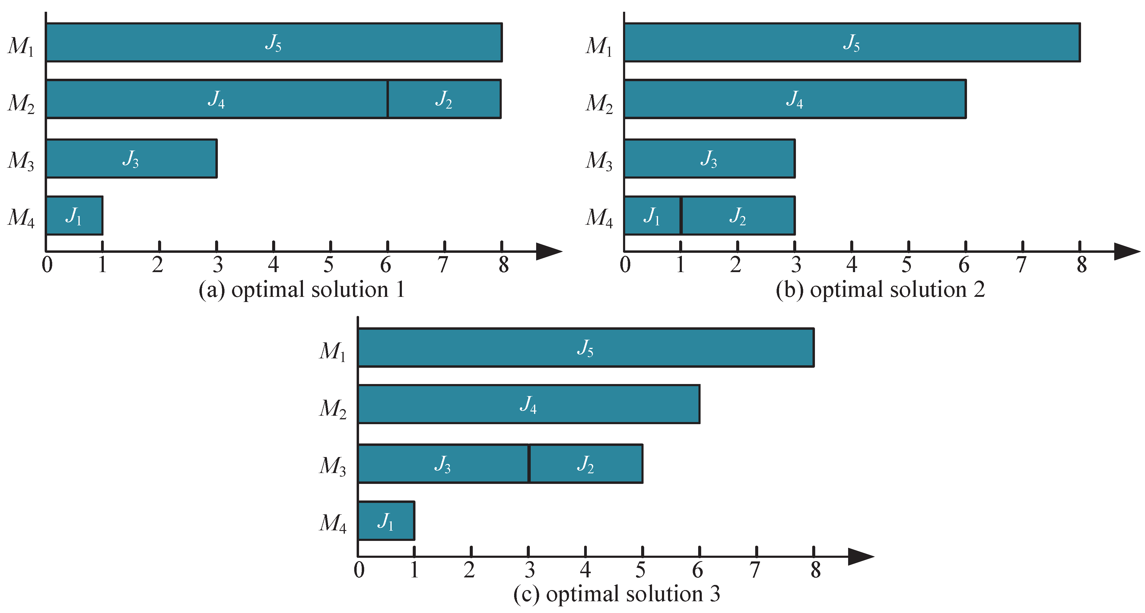
Figure 1. Illustration of three optimal solutions to Example 1 for problems P m | | C max and P m | | A R P I .
Applsci 13 08720 g001
Figure 2. Illustration of two optimal solutions to Example 2 for problem P m | | M W D .
Applsci 13 08720 g002
Figure 3. Illustration of an optimal solution to problem P m | | S I .
Applsci 13 08720 g003
Figure 4. Illustration of a chromosome.
Applsci 13 08720 g004
Figure 5. The framework of the I L S A L P T algorithm.
Applsci 13 08720 g005
Figure 6. The feasible solutions obtained by L S A L P T and I L S A L P T .
Applsci 13 08720 g006
Table 1. Experimental results of small job instances with job processing time range from 5 to 10.
(m, n)CPLEX LSA RPT LSA LPT LSA SPT GA BM ILSA LPT
obj gap 1 obj gap 1 obj gap 1 obj gap 1 obj gap 1
( 2 , 5 ) 6.74 7.85 16.47 7.36 9.20 8.51 26.26 6.74 0.00 6.74 0.00
( 2 , 10 ) 6.72 7.11 5.80 6.74 0.29 7.06 5.06 6.72 0.00 6.74 0.30
( 2 , 15 ) 6.79 7.03 3.53 7.60 11.93 8.64 27.25 6.79 0.00 6.80 0.15
( 3 , 5 ) 11.19 12.09 8.04 11.19 0.00 12.21 9.12 11.19 0.00 11.19 0.00
( 3 , 10 ) 10.29 10.75 4.47 11.04 7.29 11.84 15.06 10.29 0.00 10.32 0.29
( 3 , 15 ) 11.00 11.55 5.00 11.00 0.00 11.19 1.73 11.00 0.00 11.00 0.00
( 4 , 5 ) 13.89 14.15 1.87 13.89 0.00 14.72 5.98 13.89 0.00 13.89 0.00
( 4 , 10 ) 13.77 14.77 7.26 14.53 5.52 15.39 11.76 13.77 0.00 14.09 2.32
( 4 , 15 ) 14.37 15.76 9.67 14.97 4.18 15.79 9.88 14.37 0.00 14.46 0.63
Average 10.53 11.23 6.90 10.92 4.27 11.71 12.46 10.53 0.00 10.58 0.41
Note: g a p 1 = o b j o b j * o b j * × 100 % , where o b j * is the exact solution obtained by CPLEX.
Table 2. Experimental results of large job instances with job processing time range from 5 to 10.
(m, n) LSA LPT LSA RPT LSA SPT GA BM ILSA LPT
obj * * Time (s) obj Time (s) gap 2 obj Time (s) gap 2 obj Time (s) gap 2 obj Time (s) gap 2
( 3 , 50 ) 12.11 <1 11.80 <1 2.56 12.99 <1 7.27 11.44 1 5.53 11.45 <1 5.45
( 3 , 100 ) 12.19 <1 12.50 <1 2.54 13.12 <1 7.63 11.49 1 5.74 11.49 <1 5.74
( 3 , 500 ) 12.23 <1 12.28 <1 0.41 13.07 <1 6.87 11.53 3 5.72 11.53 <1 5.72
( 3 , 1000 ) 12.24 <1 11.77 <1 3.84 13.13 <1 7.27 11.54 5 5.72 11.54 <1 5.72
( 5 , 50 ) 17.71 <1 18.26 <1 3.11 18.01 <1 1.69 17.72 2 0.06 17.71 <1 0.00
( 5 , 100 ) 17.84 <1 18.78 <1 5.27 18.09 <1 1.40 17.85 2 0.06 17.84 <1 0.00
( 5 , 500 ) 17.87 <1 18.99 <1 6.27 18.14 <1 1.51 17.88 4 0.06 17.87 <1 0.00
( 5 , 1000 ) 17.87 <1 18.68 <1 4.53 18.16 <1 1.62 17.89 6 0.11 17.87 <1 0.00
( 15 , 50 ) 36.98 <1 36.76 <1 0.60 38.68 <1 4.60 36.43 5 1.49 36.10 <1 2.38
( 15 , 100 ) 36.88 <1 37.07 <1 0.52 38.40 <1 4.12 36.20 4 1.84 35.84 <1 2.82
( 15 , 500 ) 37.25 <1 37.56 <1 0.83 38.78 <1 4.11 36.60 7 1.75 36.12 <1 3.03
( 15 , 1000 ) 37.27 <1 37.48 <1 0.56 38.80 <1 4.11 36.56 9 1.91 36.13 <1 3.06
( 20 , 50 ) 43.51 <1 43.34 <1 0.39 45.03 <1 3.49 42.76 5 1.72 43.01 <1 1.15
( 20 , 100 ) 42.38 <1 43.46 <1 2.55 42.86 <1 1.13 43.13 6 1.77 42.38 <1 0.00
( 20 , 500 ) 42.44 <1 43.73 <1 3.04 42.93 <1 1.15 43.03 8 1.39 42.44 <1 0.00
( 20 , 1000 ) 42.46 <1 43.98 <1 3.58 42.93 <1 1.11 43.09 11 1.48 42.46 <1 0.00
Average 27.45 <1 27.90 <1 1.61 28.32 <1 3.69 27.20 5 1.66 26.99 <1 2.19
Note: g a p 2 = o b j o b j * * o b j * * × 100 % .
Table 3. Experimental results of large job instances with job processing time range from 8 to 10.
(m, n) LSA LPT LSA RPT LSA SPT GA BM ILSA LPT
obj * * Time (s) obj Time (s) gap 2 obj Time (s) gap 2 obj Time (s) gap 2 obj Time (s) gap 2
( 3 , 50 ) 13.24 < 1 13.06 < 1 1.36 13.70 < 1 3.47 11.53 1 12.92 11.53 < 1 12.92
( 3 , 100 ) 13.23 < 1 12.55 < 1 5.14 13.65 < 1 3.17 11.51 1 13.00 11.52 < 1 12.93
( 3 , 500 ) 13.26 < 1 12.73 < 1 4.00 13.68 < 1 3.17 11.54 3 12.97 11.54 < 1 12.97
( 3 , 1000 ) 13.26 < 1 12.78 < 1 3.62 13.68 < 1 3.17 11.54 5 12.97 11.54 < 1 12.97
( 5 , 50 ) 17.83 < 1 18.19 < 1 2.02 17.88 < 1 0.28 17.83 2 0.00 17.83 < 1 0.00
( 5 , 100 ) 17.83 < 1 18.26 < 1 2.41 17.87 < 1 0.22 17.83 2 0.00 17.83 < 1 0.00
( 5 , 500 ) 17.88 < 1 19.14 < 1 7.05 17.93 < 1 0.28 17.88 4 0.00 17.88 < 1 0.00
( 5 , 1000 ) 17.88 < 1 18.87 < 1 5.54 17.93 < 1 0.28 17.89 6 0.06 17.88 < 1 0.00
( 15 , 50 ) 38.86 < 1 38.25 < 1 1.57 39.67 < 1 2.08 37.93 4 2.39 37.32 < 1 3.96
( 15 , 100 ) 38.94 < 1 38.28 < 1 1.70 39.63 < 1 1.77 37.84 4 2.83 36.56 < 1 6.11
( 15 , 500 ) 38.96 < 1 37.52 < 1 3.70 39.70 < 1 1.90 37.37 6 4.08 36.12 < 1 7.29
( 15 , 1000 ) 38.97 < 1 37.37 < 1 4.11 39.73 < 1 1.95 37.20 10 4.54 36.13 < 1 7.29
( 20 , 50 ) 46.07 < 1 45.81 < 1 0.56 46.84 < 1 1.67 45.31 5 1.65 44.86 < 1 2.63
( 20 , 100 ) 42.43 < 1 42.78 < 1 0.82 42.51 < 1 0.19 42.64 6 0.49 42.43 < 1 0.00
( 20 , 500 ) 42.47 < 1 43.89 < 1 3.34 42.55 < 1 0.19 43.80 8 3.13 42.47 < 1 0.00
( 20 , 1000 ) 42.47 < 1 44.15 < 1 3.96 42.55 < 1 0.19 43.93 11 3.44 42.47 < 1 0.00
Average 28.35 < 1 28.35 < 1 0.04 28.72 < 1 1.50 27.72 5 3.76 27.24 < 1 4.94
Note: g a p 2 = o b j o b j * * o b j * * × 100 % .
Disclaimer/Publisher’s Note: The statements, opinions and data contained in all publications are solely those of the individual author(s) and contributor(s) and not of MDPI and/or the editor(s). MDPI and/or the editor(s) disclaim responsibility for any injury to people or property resulting from any ideas, methods, instructions or products referred to in the content.