Novel Methodology for Scaling and Simulating Structural Behaviour for Soil–Structure Systems Subjected to Extreme Loading Conditions

Abstract

This paper is concerned with the calibration and validation of a numerical procedure for the analysis of pile performance in soft clays during seismic soil–pile–superstructure interaction (SSPSI) scenarios. Currently, there are no widely accepted methods or guidelines. Centrifuge and shaking table model tests are often used to supplement the available field case histories with the data obtained under controlled conditions. This paper presents a new calibration method for establishing a reliable and accurate relationship between full-scale numerical analysis and scaled laboratory tests in a 1g environment. A sophisticated approach to scaling and validating full-scale seismic soil–structure interaction problems is proposed that considers the scaling concept of implied prototypes as well as “modelling of models” techniques that can ensure an excellent level of accuracy. In this study, a new methodology was developed that can provide an accurate, practical, and scientific calibration for the relationship between full-scale numerical analysis and scaled laboratory tests in the 1g environment. The framework can be followed by researchers who intend to validate their seismic soil–structure interaction findings.

1. Introduction

The scale-modelling approach provides a useful means for supplementing existing data from case histories and/or prototype investigations to enable parametric studies in seismic analysis, especially when there is a dearth of available data and results. In addition to qualitative analysis, the results of scale modelling tests are frequently applied as calibration benchmarks for analytical approaches and quantitative forecasts of the prototype response. To successfully achieve this, a set of scaling relationships that can be used in the model and accurately predict the behaviour of the prototype must be developed.

In the engineering sector, it is common practice and increasingly regular to employ simulations and computational tools to model situations in which physical testing is impractical or prohibitively expensive. It is customary to make assumptions to precisely define the system, commonly referring to the resulting system as an idealised prototype. The assumptions made during the initial stages are usually only imposed to ensure a clear and well-defined problem.

In geotechnical engineering, the use of scale models enables the controlled modelling of complicated systems and offers the opportunity to understand the fundamental mechanisms involved in operating these systems. In certain situations, such as a static lateral pile loading test, a scale-modelled test can provide an effective alternative to the corresponding full-scale test. In investigations of dynamic soil–pile interaction, the scale modelling test allows the simulation of cases that can never be accomplished in a full-scale prototype [1]. In this context, the main aim of this paper was to develop and validate a practical technique for the scaling of dynamic soil–structure interaction problems. A novel, scaled testing technique was developed together with a calibration method for establishing the relationship between full-scale numerical analysis and scaled laboratory tests in a 1g environment, and both are described in detail.

First, the theories and background relating to the scale-modelling approach are described, and the development of scale modelling criteria for shaking table tests is explored. Then, the adoption of scaling criteria and the design of the soil and pile models are explained. The subscale models are examined to predict the behaviour of prototype materials using a sophisticated scaling approach. The results are then validated through comparison with the results from a series of physical shaking table experiments [2]. Once the scaled approach is validated and the relationship between the experimental data and the results of the full-scale numerical analysis for the prototype system is determined, the new practical technique for the scaling and validation of dynamic soil–structure interaction problems is presented.

2. Background of Scale Model Similitude Theories

The relation between a scaled model and the analogous prototype behaviour can be characterised using the theory of “scale model similitude”. Ref. [3] described three different approaches with varying levels of sophistication, including “dimensional analysis theory”, “similitude theory”, and “governing equations method”. Dimensional analysis theory is based on the principle of dimensional homogeneity [4]. This theory involves transforming the homogeneous equations dimensionally, comprising the quantities physically, and defining a physical circumstance as a corresponding equation involving dimensionless products of powers of the physical quantities. Dimensional analysis theory can be employed to understand the problem–solution form without the direct application of scale modelling. Similitude theory, on the other hand, involves setting up the necessary and appropriate conditions for correlation between phenomena. This approach can accurately predict the behaviour of a prototype by using scaling laws related to the prototype through similarity conditions, as schematically illustrated in Figure 1 [5,6,7].

“Similitude theory” pinpoints the forces functioning in a system and employs dimensional analysis to form and associate the dimensionless terms for the scale model and full-scale prototype [8]. The prediction equations are commonly referred to as the scaling relationships that exist between the model and the prototype. Finally, the governing-equations method comprises changing the differential equation characterizing the process to a nondimensional equation and developing similarity between the model and the prototype variables, including the initial and boundary conditions of the system. In addition, it is imperative to establish similarity variables for the initial and boundary conditions that govern the system.

Scale models of dynamic loading and soil–structure interaction (SSI) conditions can be described as those involving geometric, kinematic, and dynamic similarities to the prototype [9]. Geometric similarity describes a situation wherein the model and the prototype have analogous physical dimensions. Kinematic similarity refers to a phenomenon in which the model and the prototype have analogous particles at similar points and times, whilst dynamic similarity defines a circumstance in which corresponding components of both the model and prototype undergo analogous forces. Scale models may fulfil the criteria of similarity to the prototype with different degrees of accuracy. The terms “distorted”, “adequate”, and “true” are sometimes used to describe the degree of accuracy with regard to meeting the requirements of similitude [10]. A “distorted” model is a scale model in which the prediction equation is distorted due to a significant deviation in similitude requirements. Compensating distortions are introduced to preserve the prediction equation in other dimensionless products. A scale model is “adequate” when the primary features of the phenomenon are correctly scaled with minor deviation consequences and the equation of prediction is not considerably influenced. A “true” model refers to a scale model that fulfils all similitude requirements.

Dimensional analysis essentially intends to reduce the number of parameters in a model to the fundamental “measures of nature”, i.e., mass, length, and time, while developing a scale factor for all three quantities. For instance, the modulus of elasticity is a stress indicator with units of force/area and corresponding dimensions of $M{L}^{-1}{T}^{-2}$, which represent the mass (M), length (L), and time (T) dimensions. Therefore, the scale factors for mass $\mu$, length $\lambda$, and time $\tau$ can be combined to develop a scaling relation of $\mu {\lambda }^{-1}{\tau }^{-2}$, which correlates the model–prototype stress response. As strain is a dimensionless parameter, the scaling relation between the model and prototype strains is 1:1. The densities $\rho$ of the materials in the model ${\rho }_{model}$ and the prototype ${\rho }_{prototype}$ are ordinarily applied as a basis for defining the relationship between scale factors $\mu$ and $\lambda$. $\mu$, $\lambda$, and $\tau$ can be expressed in accordance with Equations (1)–(3), respectively:

$$\frac{L_m}{L_p}=\lambda$$

(1)

$$\frac{M_m}{M_p}=\mu$$

(2)

$$\frac{T_m}{T_p}=\tau$$

(3)

In these expressions, the subscripts for M, L, and T correspond to the model (m) and prototype (p), respectively. Following on from this, the ratio of the model density (ρ_model) to the prototype density (ρ_prototype) equals unity when the following criteria is satisfied:

$$\frac{{\rho }_{model}}{{\rho }_{prototype}}=1=\frac{M_m}{M_p} · \frac{V_p}{V_m}$$

Once $\frac{M_m}{M_p}$ is $\mu$ and $\frac{V_p}{V_m}=\frac{1}{{\lambda }^3}$, $\mu$ can be computed as ${\lambda }^3$.

The time scale factor $\tau$ can be computed using the equation of the inertial force ratio, in accordance with Equations (4)–(7), where $A_m$ and $A_p$ represent the areas of the model and prototype, respectively, and ${\gamma }_m$ and ${\gamma }_p$ are the corresponding model and prototype unit weights:

$$\left(\frac{M_m{A}_m}{M_p{A}_p}\right)=\left(\frac{{\gamma }_m}{{\gamma }_p}\right)·{\lambda }^3·\left(\frac{A_m}{A_p}\right)$$

(4)

with the weight ratio given as:

$$\left(\frac{{\gamma }_m}{{\gamma }_p}\right)·{\lambda }^3$$

(5)

The model accelerations must be equal to the prototype accelerations, and thus:

$$\left(\frac{A_m}{A_p}\right)=1=\frac{\left(\frac{L_m}{T_m^2}\right)}{\left(\frac{L_p}{T_p^2}\right)}=\frac{L_m}{L_p}·\frac{T_p^2}{T_m^2}=\lambda ·{\left(\frac{T_p}{T_m}\right)}^2$$

(6)

in which

$$1=\lambda ·{\left(\frac{T_p}{T_m}\right)}^2, \lambda ={\left(\frac{T_m}{T_p}\right)}^2$$

(7)

where $\tau =\frac{T_m}{T_p}$. $\tau$ can then be computed as equal to ${\lambda }^{\frac{1}{2}}$.

Through the determination of scaling factors for mass (μ), length (λ), and time (τ) in relation to λ, it is possible to establish a comprehensive set of scaling relationships that are dimensionally accurate for all variables under investigation. The earthquake resistance of rock-filled dams and sloping core dams was examined by Clough and Pirtz (1956) [11], and Clough and Seed (1963) [12] respectively, through the utilisation of scale models in their methodology. One limitation of this methodology is that it treats each variable in isolation, disregarding its system function. A methodology of dimensional analysis involves the Buckingham $\pi$ theorem approach of scale model. According to this theorem, “any dimensionally homogeneous equation involving certain physical quantities can be reduced to an equivalent equation involving a complete set of dimensionless products” [13]. Consequently, the solution for a studied physical quantity of interest $\left(X_1,X_2, \dots , X_n\right)$ can be expressed as given in Equation (8):

$$F\left(X_1,X_2, \dots , X_n\right)=0$$

(8)

and stated in the form of $\pi$, as given in Equation (9):

$$G\left({\pi }_1,{\pi }_2, \dots , {\pi }_{\eta }\right)=0$$

(9)

In this expression, $\pi$(s) denotes the autonomous dimensionless products of the physical quantities $X_1,X_2, \dots , X_n$; the symbol η represents the count of dimensionless products; while $n$ signifies the quantity of physical variables. The relation between these two terms is expressed in Equation (10):

$$\eta =n-\mathrm{t}\mathrm{h}\mathrm{e} \mathrm{n}\mathrm{u}\mathrm{m}\mathrm{b}\mathrm{e}\mathrm{r} \mathrm{o}\mathrm{f} \mathrm{i}\mathrm{n}\mathrm{v}\mathrm{o}\mathrm{l}\mathrm{v}\mathrm{e}\mathrm{d} \mathrm{f}\mathrm{u}\mathrm{n}\mathrm{d}\mathrm{a}\mathrm{m}\mathrm{e}\mathrm{n}\mathrm{t}\mathrm{a}\mathrm{l} \mathrm{m}\mathrm{e}\mathrm{a}\mathrm{s}\mathrm{u}\mathrm{r}\mathrm{e}\mathrm{s}$$

(10)

The process of establishing of individual π terms involves the classification of physical variables into dimensionless quantities. It is imperative to incorporate all of the variables while ensuring that the term $m$ remains independent. Theoretically, for a given scale-modelling issue, there is no unique set of $\pi$, but the variables should be correctly identified, and $\pi \left(s\right)$ should be constructed correctly. The scaling relationships may then be established by connecting the model ${\pi }_{i,m}$ to the corresponding prototype ${\pi }_{i,p}$, where $i$ ranges between 1 and η. As stated earlier, the similitude theory endeavours to realistically characterise the problem by devising π term forms that are grounded in the prevailing forces in the system [10]. The stress components of the time history ${\sigma }_{ij}\left(r,t\right)$ for a scale model are evaluated by analysing the formation of π terms resulting from an imposed acceleration time history $a\left(t\right)$, where i, j = 1, 2, 3, etc. In order to satisfy the criteria for (true) scale modelling, it is imperative to adhere to two fundamental requirements, namely the Froude and Cauchy conditions. The indicated stress is a function of a number of variables involved in the system (see Equation (11)). Subsequently, the $\pi$ terms can be developed as given in Equation (12).

$$\sigma =F(r,t,\rho ,E,a,g,l,{\sigma }_o,r_o)$$

(11)

$$\frac{\sigma }{E}=\left(\frac{r}{l},\frac{t}{l},\sqrt{\frac{E}{\rho }},\frac{a}{g} ,\frac{gl\rho }{E},\frac{{\sigma }_o}{E},\frac{r_o}{l}\right)$$

(12)

In these equations, the variables $r,t,\rho ,E,a,g,l,{\sigma }_o,\mathrm{a}\mathrm{n}\mathrm{d} r_o$ represent the position, time, material density, elastic modulus, acceleration, acceleration of gravity, object length, initial stress, and initial position, respectively. In 1g scale modelling, the dimensionless product $a/g$ and Froude’s number ${ v}^2/lg$ must be equal to unity, which means that the model–prototype ratio of a specific stiffness $\left(E/\rho \right)$ is equivalent to the geometric scaling factor $\lambda$. This is referred to as the Cauchy condition and may be expressed in terms of the shear wave velocity ($V_S$):

$$\left(\frac{{\left(V_S\right)}_m}{{\left(V_S\right)}_p}\right)=\sqrt{\lambda }$$

(13)

Moncarz and Krawinkler (2006) [10], also showed that in a dynamic model system, the Cauchy condition is an essential requirement for synchronous replication of restoring, inertial, and gravitational forces. However, the challenge in designing a true scale model is in selecting the model materials to satisfy the Cauchy condition with an amalgamation of a small elastic modulus and a large density. Alternatively, Moncarz and Krawinkler (2006) proposed two alternatives to perform scale-modelling tests; these included simulating the artificial mass and ignoring gravitational effects.

2.1. The Concept of Application of Scale Model Similitude to Soil Mechanics

The scale modelling of geotechnical problems was initially described by Rocha (1958) [14] who differentiated between total and effective stress and also developed independent similarity relationships for each situation. For scale modelling to be employed in different types of stress system in a 1g scale model, this approach assumes a linear stress–strain relation between the model and prototype. Accordingly, the soil constitutive model can be scaled. This hypothesis is shown in Figure 2, where $\alpha$ and $\beta$ represent the stress and strain scaling factors, respectively. The scaling of strain conflicts with the underlying philosophy of the dimensional analysis method. However, the restriction of derivations within elastic deformations is justified by the analysis becoming insurmountably complicated once the nonlinear response is considered.

Roscoe (1968), [15], examined the complexity of replicating the constitutive behaviour of a prototype in scale models for soils whose response hinges on the confining pressure loading condition, i.e., soil self-weight. The assumptions adopted by Rocha (1958) were extended such that the strain behaviours of the scaled and prototype elements of a soil are assumed to be identical only if these components are subjected to two geometrically comparable stress paths (provided that their initial states in the $\mathrm{e}-\mathrm{l}\mathrm{n}{\mathsf{\sigma }}^{\prime }$ relation are equidistant from the critical state line). This hypothesis is demonstrated in Figure 3 and has been validated by a limited number of physical tests. Roscoe also asserted that a centrifuge programme is an applicable approach for this type of scaling method.

In further developments, the “Buckingham pi theorem” was developed in 1986 to solve the scale-modelling problem of the dynamic interaction of a pile in clay soil [16]. A nondimensional equation was developed to define this theory; with reference to Figure 4, $D,EI, \mathrm{a}\mathrm{n}\mathrm{d} M$ are reference parameters in accordance with Equation (14):

$$\frac{x}{D}=f\left(\frac{y}{D}, \frac{M_c}{D{M}_p},\frac{J_c}{D^3{M}_p},\frac{M_p}{\rho D^2},\frac{EI}{E_r{D}^4},\frac{EI}{E_l{D}^4},\frac{F{D}^2}{EI},\frac{M_p{D}^4{\omega }^2}{EI},\omega T_O,\frac{{\omega }^{2}D}{g}\right)$$

(14)

where $x$ is the pile lateral displacement,$y$ is the y-coordinate of maximum lateral deflection, $D$ is the pile diameter, $M_c$ is the pile cap mass, $M_p$ is the pile mass per unit length, $J_c$ is the moment of inertia of the pile cap, $\rho$ is the soil mass density, $E$ is Young’s modulus of the pile, $I$ is the moment of inertia of the pile section, $E_r$ is the soil storage modulus, $E_l$ is the soil loss modulus, $F$ is the applied lateral load, $\omega$ is frequency of vibration, $T_o$ is the linear frequency sweep period, and $g$ is the acceleration of gravity, which indicates the necessity for significant gravity in the last term.

Kana et al. (1986) [16] concluded that the gravity effects for the lateral pile response for overconsolidated clay were negligible, so the experiments were performed within this scaling system and in a 1g environment. The results demonstrated that the gravitational effects for these particular test conditions were insignificant. The frequency response was predominantly dependent on the material properties of the soil and piles. Gohl (1991) [18], also employed “dimensional analysis” to develop the functional relation given in Equation (15) for scale model similarity, which is used in shaking table tests to evaluate the effects of soil–pile interaction for several intensities of shaking:

$$\frac{y}{b}=K\left(\frac{l}{u_o},\frac{{\rho }_p}{{\rho }_s},\frac{EI}{G_s{u}_o^4},\frac{{\omega }^2{u}_o}{g},\frac{m_o}{{\rho }_s{u}_o^3}\right)$$

(15)

In this expression, $y$ is the lateral displacement of the pile, $b$ is the pile diameter, $l$ is the pile length, $u_{o }$ is the input motion amplitude (applied at the base of the model), ${\rho }_p$ is the pile density, ${\rho }_{s }$ is the soil density, $EI$ is the flexural rigidity of the pile, $G_s$ is the shear stiffness of the soil (which depends on depth and strain), $\omega$ is the natural frequency of input motion, $g$ is the acceleration of gravity, and $m_o$ is the superstructure mass. Gohl (1991) found that fulfilling the second and third scaling laws simultaneously is challenging. The former entails identical model and prototype material densities, while the latter yields a prototype-to-model pile flexural rigidity ratio of ${\lambda }^5$. In order to tolerate imperfect model similarity, tests must be viewed as prototype cases against which analytical simulations can be validated. In addition, it was indicated that test results can be depicted in terms of dimensionless variables in order to facilitate comparisons with data from large-scale tests.

Iai (1989) [17], developed a scale model for a shaking table test designed to simulate the constitutive behaviour of saturated soils by considering a tangent modulus method based on the results published by Rocha (see Figure 4). A set of scaling relationships for the soil–structure–fluid interaction system subjected to dynamic loading was derived whereby the scaled dynamic problem was defined in terms of geometric, density, and strain scaling factors. The methodology prescribes the geometric ($\lambda$) and density (${\lambda }_{\rho }$) scaling factors; the strain scaling factor (${\lambda }_{\epsilon }$) is then derived using shear wave velocity tests for the prototype and model of the soil, as given in Equation (16):

$${\lambda }_{\epsilon }=\frac{\lambda }{{\left(\frac{{\left(V_S\right)}_p}{{\left(V_S\right)}_m}\right)}^2}$$

(16)

A counterintuitive consequence in this approach is that quantities for a particular model with the same dimensions may have distinct scaling factors such as length and deflection. Nevertheless, this technique has been validated through comparison with laboratory tests. According to Iai (1989) [17], this approach is only applicable for low-strain circumstances, and the soil particles remain in contact but continue to contribute to the liquefaction issue involving medium to dense sand soil deposits.

In another approach, Scott (1989) [19] employed the governing equations for dynamic equilibrium in order to develop scaling factor relationships for the soil model in centrifuge testing. This derivation was further refined by Gibson (1997) [20], such that it can be employed for a granular saturated soil subjected to a centrifuge modelling programme or a 1g environment. The expression for the developed relationships is given as:

$$\left(1-\frac{x^{\ast }}{{\sigma }^{\ast }}·\frac{x^{\ast }}{t^{\ast 2}}·{\rho }^{\ast }\right) {\rho }_m\left[\frac{{\partial }^2{u}_{im}}{{\partial t}_m^2}+\frac{{\partial u}_{jm}}{{\partial t}_m}·\frac{\partial }{{\partial x}_{jm}}\left(\frac{{\partial u}_{im}}{{\partial t}_m}\right)\right]=\left(1-\frac{x^{\ast }}{{\sigma }^{\ast }}·X^{\ast }\right)X_{im}$$

(17)

where x, $\sigma$, t, r, X, and * denote the stress, time, mass density, body force, and prototype-to-model ratio, respectively. In 1997, Gibson identified the dynamic behaviour of the scaling soil constitutive problem for 1g environment testing. Additionally, Gibson proposed modifications to the material properties of the model. Consequently, under 1g stress conditions, this model demonstrates strain behaviour that is comparable to that of the prototype. It applies a steady-state line as presented in Figure 5. This method is different from the approaches developed by Rocha (1958) [14], and Iai (1989) [17], which both modify the soil constitutive relationship rather than the soil material properties. It has also been observed that dynamic and diffusion time scale factors linked to pore pressure response and potential liquefaction are incompatible with 1g testing conditions unless finer grain soil and a more viscous pore liquid is used [20].

The information presented in this section highlights many important factors that are relevant to geotechnical research. The studies discussed include the crucial features of soil constitutive affinity to the set of scale-modelling demands for an accurate depiction of the soil response. The full range of nonlinear behaviour of a system must be considered, and simplifying a model to a discrete elastic parameter system is likely to provide inadequate results. Constitutive similarity is discussed in relation to the designs of the soil and pile models in Section 5 and Section 6 of this paper, respectively.

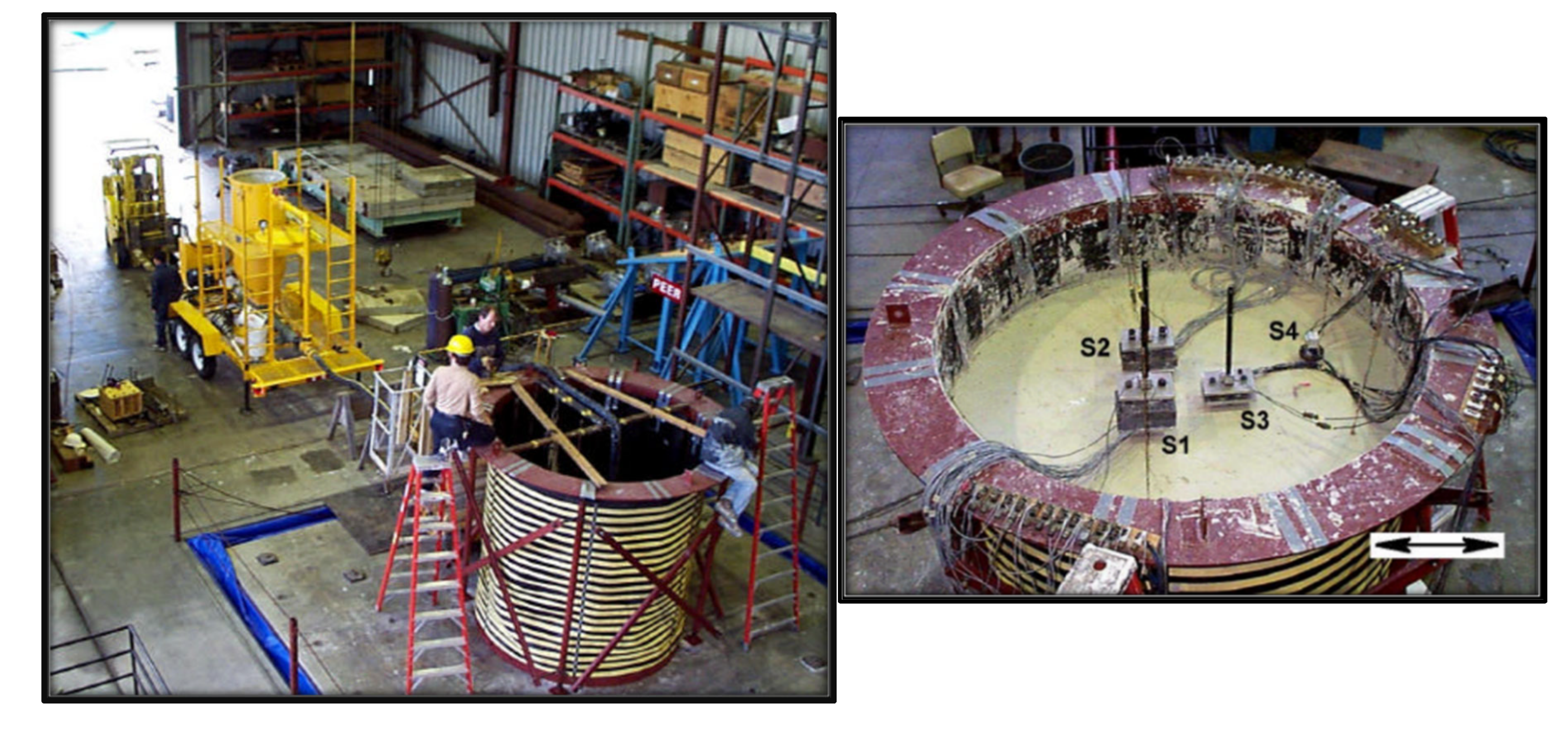
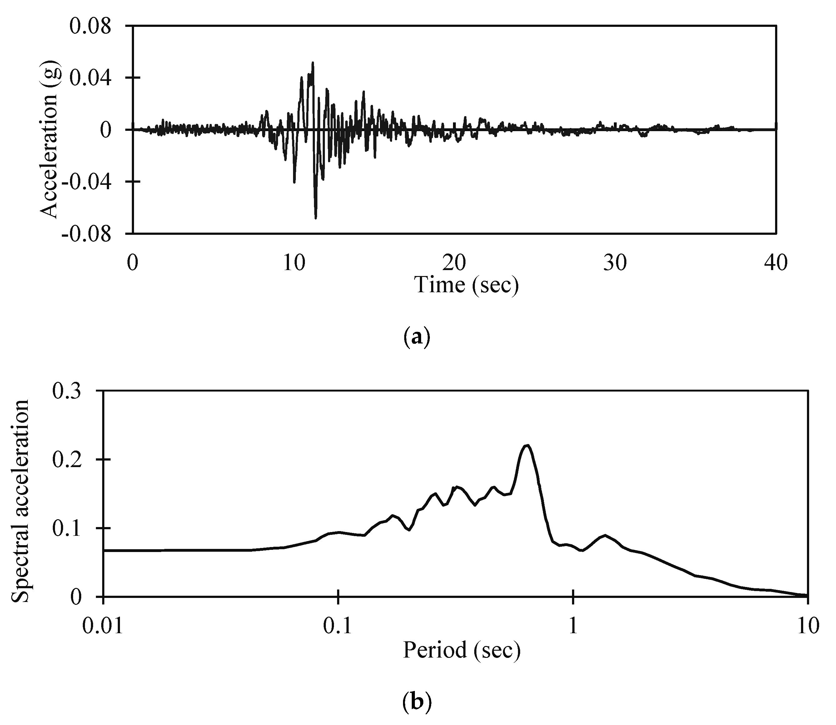
2.2. Reference Case Study

A series of physical shaking table tests comprising flexible wall barrel containers was conducted by Meymand et al. [2] at the UC Berkeley PEER Center Earthquake Simulator Laboratory [2], and the data from Phase II of this study (namely Test 1.15) was employed herein for validation of the numerical modelling. The physical specimen comprised soil that was embedded with a single pile supporting the superstructure. The experimental set-up was able to physically model the entire seismic soil–pile–superstructure interaction (SSPSI). The main aim of the experimental campaign was to provide an insight into specific SSPSI issues such as the frequency response of the structure, multidirectional excitation, kinematic and inertial responses, and pile soil contact. The individual model piles were tested simultaneously and arranged in the test container in a manner that minimised element interactions [21].

In terms of instrumentation, there were twenty-three accelerometers arranged in two vertical arrays embedded in the soil deposit that were attached to the head masses of the piles to capture translation and rocking motions. In addition, seven pairs of strain gauges were attached to each pile. Based on the soil strength and shear wave velocity profiles, the soil in the tests was defined as being lightly overconsolidated soft to medium stiff clay. The shaking table employed in the physical reference case study tests was 6.1 m × 6.1 m in plan and had a load capacity of 580 kN, a frequency range of 0–20 Hz, and six controlled degrees of freedom [2]. In a geotechnical scaled/SSPSI problem, a container is typically used to confine the soil and to impose boundary conditions that may not occur in the prototype full-scale field scenario. Accordingly, in these tests, a suitable container was designed that could minimise the effect of free boundary conditions on the overall system response and also enable the model to replicate the seismic behaviour at the level ground. On this basis, a laterally flexible and radially stiff cylindrical container was selected for the quasi-free field response. This design extended the centrifuge testing laminar box concept to permit multidirectional excitation [22].

The container constrained a soil column that was 2.3 m in diameter and 2.0 m in height and installed on the surface of the shaking table, as shown in Figure 6. The top steel ring was supported by four steel pipe columns connected by heavy-duty universal joints, which allowed the ring full translational freedom but prevented overturning rotations. The flexible wall of the container comprised a neoprene rubber membrane that was 6.4 mm thick that was suspended from the top ring and fastened at the base. The flexible wall was confined by a set of woven Kevlar straps that were 45 mm in width and arrayed in circumferential bands around the exterior of the membrane and arranged at intervals of 60 mm. The elastic modulus E of the combined membrane was designed to be identical to that of the soil to ensure that the free-soil boundary condition was not affected. The combination of the rubber membrane and the set of straps provided lateral flexibility and radial stiffness for the container boundary conditions. A plastic sheet sealed the top of the soil specimen during the period between tests, and water was sprayed on top of the soil to prevent the soil surface from drying out. For each test series, the pile was driven into the soil. The model was left for approximately five days before performing the next test due to the beneficial effects of soil thixotropy.

In Test 1.15, a set of single-pile models with head masses of 3.0, 11.40, 45.4, and 72.70 kg were studied, and the system was subjected to unidirectional shaking. The input was taken from the seismic event of the 90-degree component from the Yerba Buena Island record during the Loma Prieta Earthquake (YBI90)—its acceleration time history, and acceleration response spectrum are shown in Figure 7. The YBI90 record had a predominant period of 0.67 s, a time step of 0.02 s, and a PGA of 0.07 g, which for this physical and numerical testing programme was scaled to 0.2 g to provide the medium level of excitation [23]. In accordance with the scaling relations given in Table 2 in Section 3, the time steps of the input motion were divided by ${\lambda }^{0.5}$ in both the physical and numerical models, resulting in compressed time scales compared with the original records.

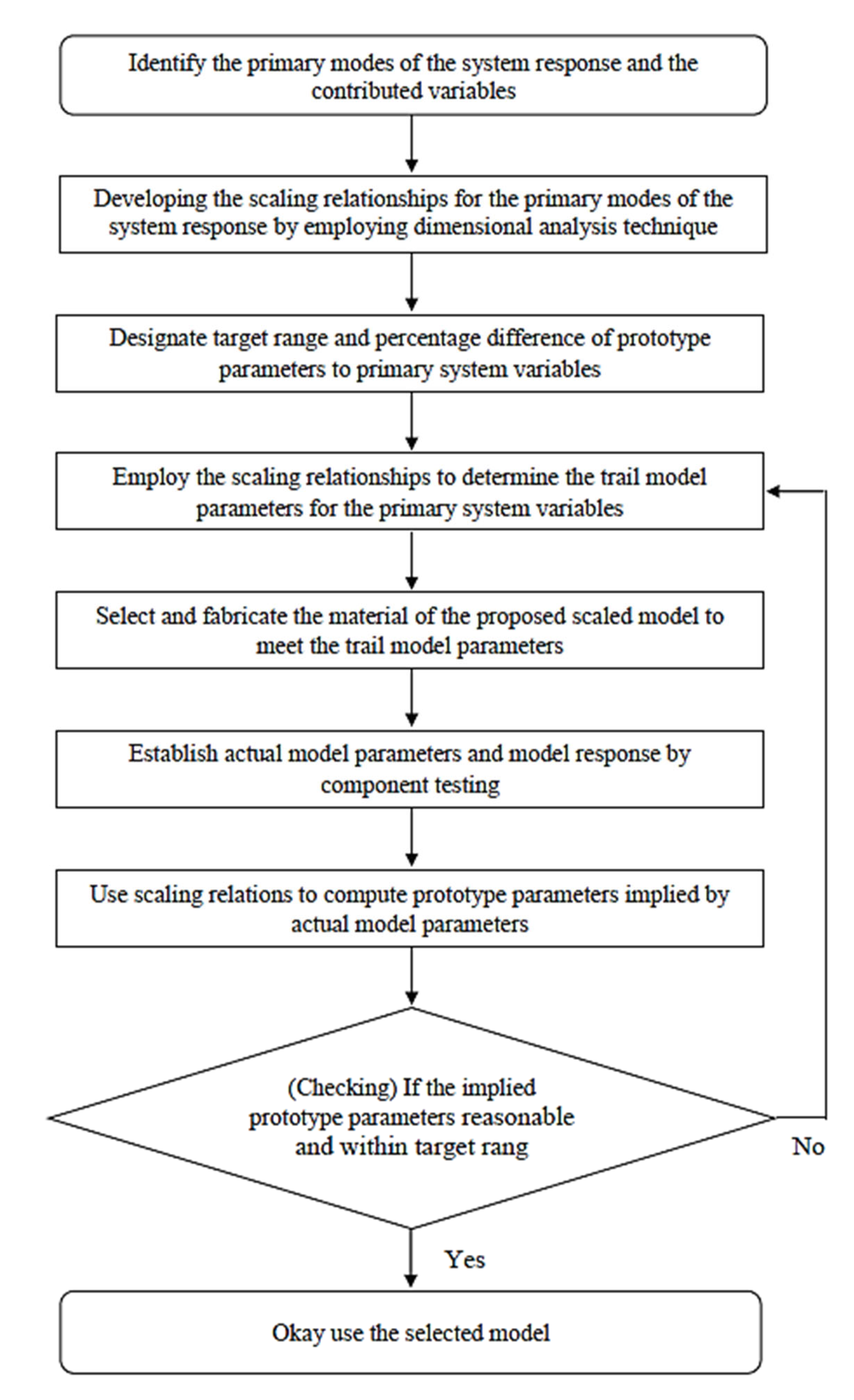
3. Implied Prototype Scaling Methodology

3.1. General

The interdependent processes of a seismic soil–pile–structure interaction (SSPSI) problem and its components constitute an important part of the scale-modelling approach in which the variables and modes of the system are defined. The design of the scale model programme must be developed to enable the system to capture the behaviour(s) of principal interest adequately. It is not possible to derive a single governing equation to describe a full-scale SSPSI system. Equally, neither similitude theory nor dimensional analysis can be directly employed to achieve “true” model similarity of this complicated system. Consequently, a viable modelling methodology involves identifying and modelling the primary forces and processes within the system successfully while suppressing the secondary effects. This scale-modelling design technique is performed as an iterative process (as shown in Figure 8).

The present methodology for scale modelling involves the preliminary identification of the fundamental modes of the system response followed by establishing the prototype values for the variables that influence these modes. The scaling relationships are utilised to ascertain the scale model parameters for the relevant variables. These relationships are derived and applied for this purpose. Subsequently, scale model components are manufactured and scrutinised to validate their performance, and scaling relationships are utilised to determine whether the model behaviour identified reflects a plausible response in a real-world scenario. The use of implied prototypes as a modelling approach is deemed suitable for a diverse array of possible soil, pile, and superstructure scenarios of the prototype. It is crucial to exercise prudence while interpreting the outcomes of the scale model test in comparison to the prototype. In the context of modelling, a more accurate application of numerical analysis involves examining the scale model instead of forecasting the performance of the inferred prototype.

The approach used to determine the precision of the scale-modelling technique is known as the “modelling of models” (e.g., [2,24]). In this technique, individual and independent tests of the same prototype are executed at various scaling factors, and the modelling technique can be considered sound if the findings consistently meet similarity requirements. Many factors must be identified throughout the entire development of the scale-modelling process, and these factors may influence the accuracy level of the scale model. Harris and Sabnis (1999) [25] addressed these factors by discussing the “accuracy and reliability of structural models” in detail. In the scale model design phase, the similitude and size consequences may influence the produced model; thus, the careful development of the scale-modelling process used for this programme is described above. In the material-fabrication phase, imperfections or overstrength may change the performance of the scale model during the test. Therefore, validation and in situ testing for the model components must be performed to verify the actual material properties. In the construction phase, the procedures for installation and application of boundary conditions may yield different stress conditions between the model and prototype. Consequently, the laboratory model should minimise the influence of boundary conditions and installation procedure. In the reference case study [2], the design of the flexible container attempted to mitigate any variability in the boundary conditions, and the model pile installation technique was designed to emulate that of the prototype.

Another possible source of error between the model and the prototype is the loading process. Nevertheless, the minor deviations between the command signal and actual input are usually negligible once the actual input signal is identified and recorded. Instrumentation defects and reading errors may arise while arranging the sensors, sensing, and/or recording data. Uncertainty evolving from the analysis of the output data is primarily due to human error. Application of the model test data to the prototype must also use scale model similitude.

As previously mentioned, the appropriate application of scale models is used to achieve insight into prototype behaviour rather than to develop an exact depiction of prototype performance. The sources of error occurring from the instrumentation compromise the inherent accuracy of the sensors and their arrangement. It is necessary to achieve high efficiency of the instrumentation to diminish this error. In the reference case study, the IC (integrated circuit) sensor accelerometers were rated with a flat response that ranged between 0 and more than 300 Hz which was beyond the frequency range of interest. The maximum nonlinearity was less than 0.2%, and the accelerometers were positioned in the soil deposit using manual surveying methods. If they were not wholly orthogonal to the shaking axis, then they might cause a noticeable reduction in output signal. Moreover, individual accelerometer arrays could have undergone small permanent movements during testing. Even a ${10}^{°}$ off-axis shift would cause a reduction in the output signal of <1.5%. According to the test environment, the installed strain gauge had a transverse sensitivity of 1.2 ± 0.2%. Other sources of possible signal distortion may include inaccurate mounting of the gauges or driving the piles in a not perfectly perpendicular line to the axis of shaking; both of these are likely to be very small and were assumed herein to be negligible. The wire potentiometers were rated with a linearity within 0.1%.

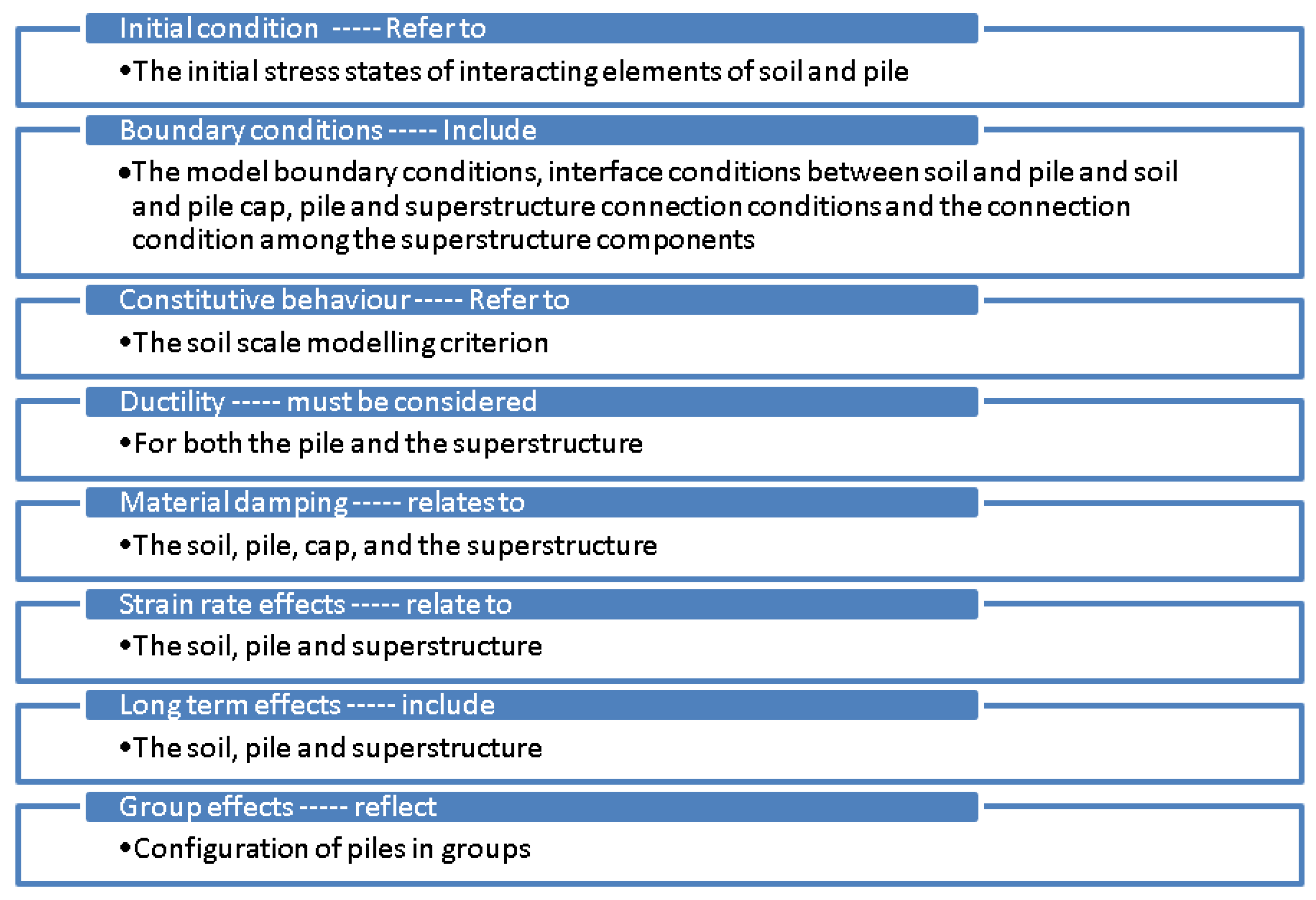
3.2. Scale-Modelling Factors

Al-Isawi et al. (2019) [21] identified various inter-related interaction modes that characterise the response of a seismic soil–pile–structure interaction system. These modes include the free-field soil site response mode, the soil–pile lateral kinematic interaction mode, the soil–pile lateral inertial interaction mode, the soil–pile axial response mode, and the pile cap radiation damping mode. The variables associated with each interaction mode are presented in

Table 1. Primary system modes and associated variables.

No.	Interaction Mode (SSPSI)	Variables
I.	Free-field	$[V_s\left(Z\right), \rho (Z),$ modulus of degradation and damping ${\left(Z\right)]}_{soil}$
II.	Soil–pile lateral kinematic interaction	$\mathrm{I}, [EI$$, \mathrm{length}, \mathrm{diameter}, \mathrm{fixity}{]}_{\mathrm{p}\mathrm{i}\mathrm{l}\mathrm{e}}$, $\left[\right(\mathrm{stress}–\mathrm{strain} \mathrm{behaviour}), {S_u\left(Z\right)]}_{soil}$
III.	Soil–pile lateral inertial interaction	$\mathrm{II}, {(M,K)}_{superstructure}$
IV.	Soil–pile axial response	$\mathrm{I}, [E,$$\mathrm{length}, \mathrm{diameter}{]}_{pile}$$,\left[\right(\mathrm{stress}–\mathrm{strain} \mathrm{behaviour}), {S_u\left(Z\right)]}_{soil}$, ${(M,K)}_{superstructure}$
V.	Radiation damping	$\mathrm{I}, (\mathrm{length}, \mathrm{diameter}, {M, E)}_{pile}$

. In this context, the objective of utilising the scale-modelling technique is to achieve what has previously been defined as dynamic similarity, whereby the scale model and prototype are subjected to comparable forces. The program relies on dimensional analysis as the fundamental principle for achieving scale model similarity. The scaling parameters are evaluated based on three primary testing criteria. Initially, the evaluation must be conducted within a 1g environment, wherein comparable model and prototype accelerations are observed. The density of the model soil and prototype soil must be comparable. This phenomenon addresses an additional element of the scaling relationships. Furthermore, it is imperative that the testing medium primarily consists of saturated clay, as its undrained stress–strain behaviour restricts pressure dependence and consequently streamlines the constitutive scaling prerequisites.

By defining the scaling conditions for the density and the acceleration, the mass, length, and time scaling factors can all be presented in terms of the geometric scaling factor λ. Then, a correct set of dimensionally accurate scaling relationships (i.e., ratio of prototype to model) for the studied variables can be derived. The scaling relationships for all of the potential variables contributing to the primary modes of system response were obtained according to the technique above and are listed in

Table 2. Scaling relationships for primary system variables.

Variable	Symbol	Factor
Mass density of saturated soil and structure	$\rho$	1
Acceleration of soil and or structure	$acce.$
Strain of soil and structure	$\epsilon$
Strain of the soil due to creep, temperature, etc.	${\epsilon }_o$
Porosity of soil	$n$
Inclination of the beam	${\theta }_{inc}$
Density of pore water and/or external water	${\rho }_f$
Inclination angle	${\theta }_{inc}$
Hydraulic gradient of external water	$i$
Length	$l$	$\lambda$
Total stress of soil and structure	$\sigma$
Effective stress of soil	${\sigma }^{\prime }$
Tangent modulus of soil	$D_T$
Bulk modulus of the solid grains of soil	$K_s$
Pressure of pore water and/or external water	$P$
Displacement of soil and/or structure	$U$
Bulk modulus of pore water and/or external water	$K_f$
Young’s modulus of the soil and structure	$E$
Shear modulus of the soil and structure	$G$
Displacement of the soil and/or the structure	$U$
Pressure of pore water and/or external water	$P$
Average displacement of pore water relative to the soil skeleton	$W$
Static soil shear strength	${S_u}_{static}$
Dynamic soil shear strength	${S_u}_{dynamic}$	$\lambda /0.75$
Time	$T_t$	${\lambda }^{\frac{1}{2}}$
Permeability of soil	$k$
Velocity of soil and/or structure	$V$
Rate of pore water flow	$W_f$
Shear wave velocity	$V_s$
Stiffness	$k$	${\lambda }^2$
Mass per unit length	${\rho }_b$
Shear force	$S_{shear}$	${\lambda }^3$
Axial force	$F_A$
Force	$F$
Mass	$\mu$
Longitudinal rigidity	$EA$
Bending moment	$M$	${\lambda }^4$
Flexural rigidity	$EI$	${\lambda }^5$
Frequency	$\omega$	${\lambda }^{-\frac{1}{2}}$

. A geometric scaling factor λ equal to 8 was selected as a benchmark for the dimensional scaling procedure, in accordance with the recommendations elsewhere [17]. A comprehensive set of scaling relationships for a soil–structure interaction system subjected to dynamic loading condition was then derived. The scaled dynamic problem was entirely defined in terms of geometric scaling factor λ. The corresponding scaling relationships for the variables that contributed to the primary system response modes were the density, acceleration, length, force, shear wave velocity, stress stiffness, time, strain, modulus, frequency, and flexural rigidity. Accordingly, when the scaling factor of the shear wave velocity equalled ${ \lambda }^{\frac{1}{2}}$, the scale model met the Cauchy condition. The calculated strain scaling factor, in accordance with Iai (1989), equalled unity. Consequently, the corresponding set of scaling relationships agreed with the values developed in the current study, as presented in Table 2.

The implementation of the scaling relationships and the creation of the components of the model soil, pile, and superstructure system are addressed in the subsequent sections of this paper. Before that, a series of definitions and assumptions that may affect the process of scale modelling and hence must be considered in the design of model components is given in Figure 9.

4. Design of the Soil and Pile Models

4.1. Soil Model

The properties of the soil model should be reflected in the primary modes of the problem behaviour and are based mainly on the type of problem being analysed. The primary modes should be first identified and then subdivided into their general categories of system behaviour to identify the system parameters that are characterised as soil properties. The dimensional scaling factor is then selected for each parameter in accordance with the data presented in Table 2. These steps are key towards achieving a “true” scale model. Following the reference case study, the five primary modes of SSPSI illustrated in Table 1 were subdivided into two general categories including the free-field site response and the soil–pile interaction. The definition of free-field site response pertains to the soil material properties and small strains, while soil–pile interaction is related to larger strains. The soil properties were defined by several parameters, including the shear wave velocity, soil density, modulus degradation and damping, stress–strain behaviour, and undrained shear strength. The parameters were both independent and nonlinear and could be expressed as a function of the loading rate, number of cycles, and strain reversals. Thus, the use of implied prototypes was suitable for the intricate modelling needed in the present study.

4.1.1. Soil-Modelling Criteria

As stated earlier, the density of the soil model was considered to be equal to the density of the prototype soil. Several other parameters such as the nonlinear stress–strain response and the modulus degradation as well as the damping curves were not explicitly modelled from the prototype case. Instead, the technique of implied prototypes was employed to determine whether the properties of the scale model for these parameters were reasonable. The undrained shear strength and shear modulus or shear wave velocity were the key parameters in the scale soil modelling. If the elastic response is required for the free-field soil and the soil–pile system, then the soil shear modulus should be modelled appropriately. On the other hand, the undrained shear strength should be modelled appropriately when the inelastic response of the soil–pile system is required. If the full nonlinear response of the dynamic system is desired, then both criteria should be considered simultaneously, as in the current study. These parameters have distinct scaling factors according to the scaling results provided in Table 2. The static and dynamic soil behaviours are affected greatly by the plasticity index (PI), which is an additional soil-modelling parameter that is not reflected in Table 1. Therefore, the use of a soil model with an analogous PI to the prototype is essential. As PI is a dimensionless parameter, a 1:1 scaling ratio between the model and the prototype was employed.

4.1.2. Prototype Soil Parameters

All of the material properties and modelling specifications were in accordance with those presented by Meymand (1998). The target prototype soil designated for the current study was the soil adopted in the reference case study, which was San Francisco Bay mud, a marine clay. This soil was suitable for the implied prototype technique and is also a well-characterised soil according to Bonaparte and Mitchell (1979), [26] who performed experiments on bay mud samples from Hamilton Air Force Base in Novato, California. The results are shown in

Table 3. Selected properties of San Francisco Bay mud, [2].

Property	Symbol	Unit	Value
Saturated unit weight	$\rho$	$\mathrm{k}\mathrm{g}/{\mathrm{m}}^3$	1505.74
Natural water content	$w_c$	%	90
Liquid limit	$LL$	%	88
Plastic limit	$PL$	%	48
Plasticity index	$PI$	%	40
Undrained strength ratio	$S_u/p^{\prime }$	Ratio	0.32
Coefficient of consolidation	$C_v$	${\mathrm{m}}^2/\mathrm{y}\mathrm{e}\mathrm{a}\mathrm{r}$	$0.743–0.930$

, which also presents the prototype parameters adopted in the current study.

Dickenson (1994), [27] investigated the seismic response of bay mud during the 1989 Loma Prieta earthquake and developed an empirical relation for expressing the undrained shear strength of the soil as a function of the soil shear wave velocity, as given in Equation (18):

$$V_s=18 {\left(S_u\right)}^{0.475}$$

(18)

where $V_s$ denotes the shear wave velocity in feet per second, and $S_u$ is the undrained shear strength in pounds per square foot. This relationship is illustrated in Figure 10 and was employed to determine the targeted shear wave velocities for the prototype soil. Appropriate shear wave velocities between 114.3 $\mathrm{m}/\mathrm{s}$ and 160 $\mathrm{m}/\mathrm{s}$ were determined for the range of prototype soil undrained shear strengths between 28.73 $\mathrm{k}\mathrm{N}/{\mathrm{m}}^2$ and 57.46 $\mathrm{k}\mathrm{N}/{\mathrm{m}}^2$, respectively.

4.2. Design of the Pile Model

The pile model was subjected to different scale-modelling criteria compared with the soil model. A successful pile model design is achieved by addressing the primary governing factors of the pile response, and the same procedure as described previously for the soil model must be applied. The primary modes should be first identified and then subdivided into their general categories of system behaviour to identify the system parameters which are characterised as soil properties. The dimensional scaling factor is then selected for each parameter in accordance with the data given in Table 2. In the case of SSPSI for the reference case study, the four principal modes of pile response were the soil–pile lateral kinematic interaction, soil–pile lateral inertial interaction, soil–pile axial response, and pile radiation damping (Table 1).

4.2.1. Pile-Modelling Criteria

There are a number of pile properties that contribute to the principal pile response modes, such as the slenderness ratio$L/d$ (where $L$ and $d$ are the pile length and diameter, respectively), flexural rigidity $EI$ (where $E$ and $I$are the pile modulus of elasticity and moment of inertia, respectively), yield behaviour, ductility, moment–curvature relationship, elastic critical buckling load $P_{cr}$, $d/t$ ratio (where t is the pile wall thickness), pile natural frequency, and the relative ground/pile rigidity. According to the scaling methodology described in Section 3, a similarity relationship for the geometry must be applied. The model properties maintain the pile slenderness and relative contact surface area, which accurately replicate the relative spacing and group interaction of the pile group in the scale model. The pile moment–curvature relationship is a principal modelling criterion because it comprises the two significant parameters—flexural rigidity and yield behaviour—that enable the fully nonlinear response of the pile under lateral loading conditions to be described.

The commonly adopted approach to achieve this involves designing piles that can respond within the elastic range while utilising the ductile behaviour of the columns in the superstructure, as suggested by Raoul et al. in 2012, [28]. The philosophy behind this approach is that it is easier to detect and repair damage to the above-ground parts of structures than it is to address damage to the subsurface parts. By utilising this method, it is possible to model the lateral dynamic response range of the pile. Scaling the pile’s flexural rigidity $EI$ and ensuring that the yield point is equal to or higher than the prototype yield point are the two ways to accomplish this. The model can accurately replicate the soil–pile kinematic and inertial interaction by scaling the resistance properties of the soil appropriately. The soil behaviour captures the nonlinear cyclic response of the pile.

The axial response of end-bearing piles is primarily influenced by the soil properties in the bearing layers, which govern the soil–pile interaction. The friction and cohesion between the soil and pile shaft as well as the elastic deformation of the pile are secondary factors that affect the axial response of an end-bearing pile. However, these factors are primarily significant for soft soil deposits. The static axial capacity of the pile is a crucial factor in determining the inertial load that the pile can carry despite the fact that axial loading is dynamic. Pile radiation damping has two behavioural components. The first component is the inherent dynamic characteristics of the pile. This refers to the pile’s ability to generate energy that can be radiated into the surrounding soil. The second component is the energy propagation away from the pile, which depends on the relative soil-pile stiffness. The relative soil–pile stiffness parameter can be automatically scaled from the prototype to the model by consistently scaling the soil and pile elastic properties. Achieving the modelling criterion for the inherent pile dynamic characteristics is a complex task. The optimisation of the natural frequency ω of an end-bearing pile can be achieved by utilising an expression that describes the natural frequency of a cantilever rod as a function of the rod’s mass $m$. This expression is given in Equation (19) and was developed by Clough and Penzien in 1995, [29].

$$\omega =3.516\sqrt{\frac{EI}{m{L}^4}}$$

(19)

As previously discussed, by scaling the pile geometry and $EI$, we can determine that the scaling factor for the mass per unit length of the model pile is ${\lambda }^2$ (refer to Table 2). It is important to examine this scaling criterion to ensure that the application conditions can accommodate conventional materials and other modelling constraints that are necessary for producing an accurate scale model. It is important to note that radiation damping has a greater impact on lower levels of shaking. However, its effect may decrease when applied to intense shaking levels in this test program. In addition, it should be noted that the pile is just one part of the soil–pile–superstructure system. Therefore, making minor adjustments to the vibration characteristics of the other components of the system is unlikely to have a significant impact on the overall vibration characteristics of the system.

4.2.2. Prototype Pile Parameters

According to the Highway Design Manual (Caltrans Standard, 2010), ref. [30] a target prototype pile is considered to be a steel pipe with a diameter of 410 mm and a wall thickness of 12.7 mm that is filled with concrete. Scaling restrictions impose a maximum prototype pile length of 12.8 m with an L/d ratio of 33, which is acceptable for a slender pile. The stability conditions of the pile, which are crucial in lateral response conditions, are as follows. The pile must be arranged as fixed against the rotation at the top and fixed against relative displacement at the base. The flexural rigidity$EI$ of the steel pipe filled with concrete is according to the reference case study (determined as 75,179 $\mathrm{k}\mathrm{N}{\mathrm{m}}^2$). The prototype pile properties yield a first mode period of vibration of 0.74 s for a cantilever rod.

4.3. Model Pile Development

An iterative process must be employed to determine the flexural rigidity $EI$and natural period in the pile design process using an appropriate laboratory test and numerical model for validation. According to the reference case study’s pile boundary condition, an equivalent cantilever rod can be used to identify the targeted principal pile parameters. A geometric scaling factor of 8 is used to develop the scaling requirements for the soil and pile models. Depending on the target model $EI$ and the scaled pile outer diameter, the moment of inertia can be computed according to two conditions; that is, for a solid and a thin-walled tube, respectively. The corresponding lower and upper bound modulus of elasticity can then be determined. The pile density is computed for both of these bounds, which then impart the scaled modes of vibration. The computed densities may range widely between two different values for solid and thin-walled sections, and these values may not be realistic for practical sections. In addition, the material type must be investigated to determine that it is appropriate as a model pile material.

In the reference case study, the target $EI$ equalled 2.3 $\mathrm{k}\mathrm{N}{\mathrm{m}}^2$ and the pile outer diameter was fixed at 50.8 mm, therefore the lower and upper bound modulus of elasticity corresponding to solid and thin tubes were 6894.76 and 68947.6 N/mm², respectively. The corresponding pile material densities were 295.30 $\mathrm{k}\mathrm{g}/{\mathrm{m}}^2$ and 573.4 $\mathrm{k}\mathrm{g}/{\mathrm{m}}^2$, respectively. Following a review of suitable materials, an aluminium 6061 T-6 alloy was selected, and the pile was designed as a thin-walled section to satisfy the $EI$criterion. Accordingly, the scale model pile was fabricated with a scaled flexural rigidity EI of 2.420 $\mathrm{k}\mathrm{N}{\mathrm{m}}^2$ and an L/d ratio of 36. The thickness of the pile wall was 0.71 mm, which is a commercially available pipe size. It is important to note that thin-walled tubes may be susceptible to local buckling, but the buckling load $P_{cr}$was found to be within the allowable range.

The theoretical moment–curvature ratio of the trial pile model must be compared to that of the prototype to ensure that the representation is appropriate. The lower and upper bound prototype scenarios were determined by employing yield stresses in the steel pipe pile of 345 and 483 N/mm², respectively, with $0\%$ and $100\%$ concrete EI contributions that represented fully intact and fully cracked concrete sections, respectively. The lower and upper bound moment–curvature relationships demonstrated at a prototype scale were defined according to the pile analysis code COM624P [31]. The results were calibrated against a four-point loading test finding performed by Caltrans on a 0.61 m concrete-filled steel pipe pile [32]. The moment–curvature relationship of the pile model can be identified using several modern approaches, and SE:MC is one of the computer programs offering this sort of analysis. SE:MC is a powerful tool for structural design and research in which moment–curvature analysis is needed and is based on a strain-compatibility technique. A numerical FEA approach was adopted for the validation process using the Abaqus software to simulate the four-point loading test. The method proposed by Langhaar (1951), ref. [33] was adopted for the determination of the moment–curvature relationship of the pile. The bending capacity equation for a ductile beam with a circular cross-section is defined as follows:

$$M=2 r^3 {\int }_0^1\beta \sigma \xi d\xi$$

(20)

where $r$ is the radius, $\beta$ represents the width of the cross section at the ordinate divided by $r$, $\xi$ represents the ordinate from the neutral axis divided by $r$, and $\sigma$ is the stress at the ordinate of the cross section. An elastic-perfectly plastic stress–strain idealisation was used to model the nominated aluminium material. Figure 11 illustrates the moment–curvature relationship for the aluminium model being tested at the prototype scale. It was observed that this relationship surpassed the yield behaviour within the desired range for the target prototype. As mentioned earlier, this outcome was acceptable since the pile was anticipated to exhibit an elastic response. A model pile material that accurately incorporated the scaled moment-curvature relationship was developed to be “optimal”. This material had a wall thickness of $5.08\times {10}^3 \mathrm{m}$, an elastic modulus of $\mathrm{20,685}$ N/mm², and a yield stress of $13.8$ N/mm².

To capture the ideal model behaviour, this material must be manufactured due to its unavailability in the market. A four-point loading test was physically examined in the reference case study, and this was replicated numerically in the current study using an Abaqus FEA model and the COM624P program with a 1.8288 $\mathrm{m}$ long and $50.8\times {10}^{-3} \mathrm{m}$diameter section of an aluminium tube with a wall thickness of $711\times {10}^{-9} \mathrm{m}\mathrm{m}$ to corroborate the model pile moment–curvature relationship. In the physical tests, foil strain gauges were positioned on the tube’s compression and tension sides and were read at each increment of loading, and the moments and curvatures were determined based on the measured strain data. This aspect was considered when the results were input into the numerical models.

The experimental moment–curvature relationship for the scale model pile is presented in Figure 12 along with the numerical data from the FEA model and the theoretical curves, all at the model scale. The agreement within the elastic response range was outstanding, and the test pile failed through a buckling mechanism that closely resembled the one depicted in the FEA and the theoretical yield point. The failure load was $725 \mathrm{N},$ which imposed a 386 Nm bending moment on the element. These tests showed that the aluminium tube was an appropriate model pile for the testing programme of the scale model.

Table 4. Input parameters of prototype pile and soil.

Prototype Input Parameters	Symbol	Value	Units
Pile outer diameter	$\mathrm{O}\mathrm{D}$	0.4064	m
Pile wall thickness	$t_{wall.p}$	$12.7\times {10}^{-3}$	$\mathrm{m}$
Pile length	$L$	$13.4112$	$\mathrm{m}$
Pile density	$\rho$	7700	$\mathrm{k}\mathrm{g}/{\mathrm{m}}^2$
Soil shear strength	${\mathrm{S}}_{\mathrm{u}}$	$25.0$	$\mathrm{k}\mathrm{N}/{\mathrm{m}}^2$
Shear wave velocity	$V_s$	$111.25$	$\mathrm{m}/\mathrm{s}$
Steel Young’s modulus	${\mathrm{E}}_{\mathrm{s}\mathrm{t}\mathrm{e}\mathrm{e}\mathrm{l}}$	$200$	$\mathrm{G}\mathrm{P}\mathrm{a}$
Concrete Young’s modulus	${\mathrm{E}}_{\mathrm{c}\mathrm{o}\mathrm{n}\mathrm{c}\mathrm{r}\mathrm{e}\mathrm{t}\mathrm{e}}$	$28$	$\mathrm{G}\mathrm{P}\mathrm{a}$
Soil Young’s modulus	${\mathrm{E}}_{\mathrm{s}\mathrm{o}\mathrm{i}\mathrm{l}}$	$28.728$	$\mathrm{M}\mathrm{P}\mathrm{a}$
Soil shear modulus	${\mathrm{G}}_{\mathrm{s}}$	163.8	MPa
Percentage of concrete EI contribution	$\mathrm{E}\mathrm{I}$	$50$	$\mathrm{\%}$

lists the input parameters of the prototype pile and soil, whilst

Table 5. Computed properties of prototype pile and soil.

Model Input Parameters	Symbol	Value	Units	Criteria
Pile outer diameter	${OD}_m$	$50.8\times {10}^{-3}$	$\mathrm{m}$	Target
Pile wall thickness	$t_{wall.p}$	$15.875\times {10}^{-4}$	$\mathrm{m}$	Target
Pile length	$L$	$1.6764$	$\mathrm{m}$	Target
$\mathrm{Pile} L/D$ Ratio	$L/D$	$33$	-	Target
Pile d/t Ratio	$d/t$	$32$	-	Target
$E_{pile}/G_{soil}$	$k$	$1392$		Target
${EI}_{pile}/E_{soil} . D^4$	$k_r$	96		Target
Soil shear strength	$S_u$	$4.167$	$\mathrm{k}\mathrm{N}/{\mathrm{m}}^2$	Target
Area of steel:	$A_{steel}$	$0.01571$	${\mathrm{m}}^2$	Scale
Steel moment of inertia	$I_{steel}$	$304.7\times {10}^{-6}$	${\mathrm{m}}^4$	Scale
$\mathrm{Steel} \mathrm{flexural} \mathrm{rigidity} EI$	${EI}_{ steel}$	60,915.6	${\mathrm{k}\mathrm{N}\mathrm{m}}^2$	Scale
Area concrete	$A_{concrete}$	0.114	${\mathrm{m}}^2$	Scale
Concrete flexural rigidity EI	${EI}_{ concrete}$	14,263.4	${\mathrm{k}\mathrm{N}\mathrm{m}}^2$	Scale
Composite concrete/steel flexural rigidity	${EI}_{ composite}$	75,179	${\mathrm{k}\mathrm{N}\mathrm{m}}^2$	Scale
Composite concrete/steel flexural rigidity	${EI}_{ composite}$	2.294	${\mathrm{k}\mathrm{N}\mathrm{m}}^2$	Target
Total Mass/m length	Ratio	397.24	$\mathrm{k}\mathrm{g}/\mathrm{m}$	Target
Prototype first mode period	$T$	0.7386	$\mathrm{s}$	Target

provides the computed properties and targeted values of the prototype pile and soil. Finally,

Table 6. Soil and pile models’ input parameters, computed properties, and percentage of result deviation from target values.

Model Parameters	Symbol	Value	Units	% Difference
Pile outer diameter	${OD}_m$	$50.8\times {10}^{-3}$	$\mathrm{m}$	Scaled
Pile wall thickness	$t_{wall.m}$	$711\times {10}^{-6}$	$\mathrm{m}$	76
Pile length	$L$	$1.8288$	$\mathrm{m}$	Scaled
Pile Young’s modulus	$E_{pile}$	$68.95$	$\mathrm{G}\mathrm{P}\mathrm{a}$	Scaled
Pile density	${\rho }_{pile .m}$	$2700$	$\mathrm{k}\mathrm{g}/{\mathrm{m}}^3$	Scaled
Soil shear strength (with 0.75 dynamic correction)	$S_u$	$4.07$	$\mathrm{k}\mathrm{N}/{\mathrm{m}}^2$	2.4
Shear wave velocity	$V_s$	$40.0$	$\mathrm{m}/\mathrm{s}$	Scaled
Pile cross sectional area	$A_{pile .model}$	$0.115\times {10}^{-5}$	${\mathrm{m}}^2$	Scaled
Pile mass/m length	Ratio	$0.07173$	$\mathrm{k}\mathrm{g}/\mathrm{m}$	Scaled
Pile moment of inertia	$I_{pile.model}$	$3.5105\times {10}^{-8}$	${\mathrm{m}}^4$	Scaled
Pile flexural rigidity/Unit length	${EI}_{pile.model}$	$2.420$	$\mathrm{k}\mathrm{N}\mathrm{m}$	$5.0$
$\mathrm{Pile} L/D$ ratio	${L/D }_{model}$	$36.0$	Dimensionless	$8.7$
Pile d/t ratio	${d/t}_{model}$	$71.4$	Dimensionless	$76$
$E_{pile}/G_{soil}$	$k_{model}$	$3840$	Dimensionless	$93$
${EI}_{pile}/E_{soil} . D^4$	$k_{r.model}$	101	Dimensionless	$5.0$

presents the soil and pile models’ input parameters, computed properties, and percentage of result deviation from target values.

5. Validation Methodology

It is very complex to conduct physical tests under dynamic loading, and they are even impossible in some circumstances such as under seismic loading, in which no fixed reference point is available to provide a reliable benchmark. All of the loading areas in a particular environment are moving during a seismic event. Therefore, most investigations performed after earthquake events are generally intended to analyse the consequences of the earthquake rather than the behaviour of the system or system component during the seismic activity. Performing an accurate large-scale laboratory test is also complicated and costly and may be impossible depending on the desired degree of complexity and accuracy. For these reasons, it can be challenging for researchers to validate their studies in seismic engineering. Utilising a scaled testing technique with a shaking table or centrifuge tests in a 1g environment is a viable (and often the only) option. Nevertheless, calibration of the results remains a significant challenge. In the current work, it was necessary to develop an accurate, practical, and scientifically acceptable calibration method for establishing the relationship between full-scale numerical analysis and the scaled laboratory tests in a 1g environment. A sophisticated and novel validation approach was developed for this purpose that is shown schematically in Figure 13. The underlying principle of the approach was based on performing two parallel analyses, i.e., a scaled physical model and a full-scale numerical model.

The first step in this process was to scale the prototype parameters using the scaling procedure described previously in Section 4. Prior to achieving the scale model, the physical test was performed according to the problem condition. The shaking table test conducted by Meymand (1998), [2] and its results were adopted in the current study as the simulated laboratory test output. After identifying the problem characteristics of the full-scale problem as a prototype that corresponded to the scale model, the full-scale numerical models using FEA were developed using similar conditions to the physical test. Once the full-scale numerical simulation was complete, the results from that analysis could be scaled according to the corresponding parameter scaling factors listed in Table 2. This step was necessary to identify all parameters involved in the final validation step. Finally, the physical shaking table experiment results were validated against the results captured from the earlier stage of this procedure.

5.1. Numerical Modelling Characteristics

A three-dimensional (3D) FEA simulation was carried out using the sequential analysis method for considering the effects of soil–structure interaction (SSI) during static and dynamic loading conditions. The sequential analysis method is commonly employed in numerical analysis for considering the consequences of the (1) geostatic, (2) static, and (3) seismic loads on a system. The first step (1) is the geostatic step, and only the soil body force is employed. Consequently, the considerable force and initial stresses should be precisely equilibrated and established for minimal soil displacement. Abaqus/Standard [34] offers two methods for establishing the initial equilibrium. The first procedure is appropriate for applications in which the initial stress state is identified approximately. The second, somewhat improved method is applicable for circumstances wherein the initial stresses are unidentified but only for a limited number of elements and materials. In this respect, the second procedure was followed in the current study, in which the pore water pressures varied linearly with depth and the initial effective stresses were appropriately stated according to the total stresses.

The second (2) step was the static step, which comprised two substeps in the analysis. Firstly, to create stability between the two interacting parts (namely, the soil and the pile) and to prevent negative shear stress between them, the static-frictionless step must be employed. This represents the piles’ installation stage during model construction. Secondly, the static-friction loading step must be applied; this comprises the application of gravity loads, which are assumed to be static and uniform, and the mass loading according to the loading condition of the physical test was also applied. In the current analysis, four pile head masses were employed as a superstructure—a set of single pile models with head masses of 3.0, 11.40, 45.4, and 72.70 kg were used in accordance with the reference physical test (Test 1.15) after applying the corresponding scaling factors as given in Table 2.

The third step (3) was the dynamic analysis step. The time history input data from the Loma Prieta earthquake, as mentioned and described previously, were applied to the bottom of the clay soil at the base of the shaking table [35]. The displacements were restrained in the horizontal direction for the geostatic and static step and changed to the vertical direction for this dynamic analysis step, allowing free movement in the horizontal direction. The base of the model was restrained with roller supports in the vertical direction. In contrast, the other two direction boundary conditions, which were perpendicular to the shaking direction, were constrained [36].

Both the soil and the superstructure were modelled using 3D solid elements (C3D8R in the Abaqus library) that were eight-node linear brick elements with reduced integration. For the piles, linear shell elements (S4R) were used; these were a four-node doubly curved shell elements [34]. As this was a cylindrical application, a radial mesh was employed in accordance with the approach of other researchers [37]. In addition, a mesh sensitivity study was conducted to achieve accurate and reliable results, resulting in elements that were 400 mm in each dimension at the boundary of the model and refined to 80 mm near and at the pile. Given the similarity between the approach of using the combination system of flexible wall material properties, which was chosen in the reference case study, and the alternative method of using the soil sample properties directly, the combination system was not adopted further in the numerical analysis. Alternatively, the soil boundary was constrained in accordance with the physical test conditions.

In the numerical model, the soil/pile contact was considered to be a discontinuous constraint, which can occur when loads transfer between contacting elements under contact conditions. In this case, once the two surfaces detached, the constraint was removed (i.e., the gap condition), and the slap condition took place during the return of the contact [38]. Accordingly, both normal and tangential behaviours were considered. Normal behaviour enabled the pressure to be transmitted between the soil and the pile, and both surfaces were in contact. This type of behaviour allowed the soil to separate when the contact pressure was reduced to zero. On the other hand, tangential behaviour enabled the shear stress (or shear drag) to transfer between the soil and the pile surface, as shown in Figure 14. Figure 15 represents the numerical model for the four piles’ head mass condition.

A fully nonlinear dynamic soil–structure interaction analysis with the application of the gap-slap mechanism was implemented in the current model by employing a Cam–clay soil constitutive model.

Table 7. Model parameters for the soil constitutive models [38].

Parameter		Value
Density (kg/m3)		1505.75
Log bulk modulus		0.05
Poisson’s ratio		0.47
Tensile limit		0.00
Log plasticity bulk modulus		0.27
Stress ratio		1.26
Wet yield surface size		1.00
Flow stress ratio		0.78
Initial void ratio		1.50
Cyclic loading parameters
Freq. (Hz)	Cyclic stress ratio (CSR)	${\xi }_{d1}$	${\xi }_{d2}$
		cyclic degradation parameters
0.1	0.6	4.2	75
0.25	0.6	4.2	97
1	0.6	4.1	420
2	0.6	4.1	600
5	0.6	4.2	825
10	0.6	4.2	1065

contains the soil constitutive models’ parameters that corresponded to the material properties of the soil used in the numerical simulation.

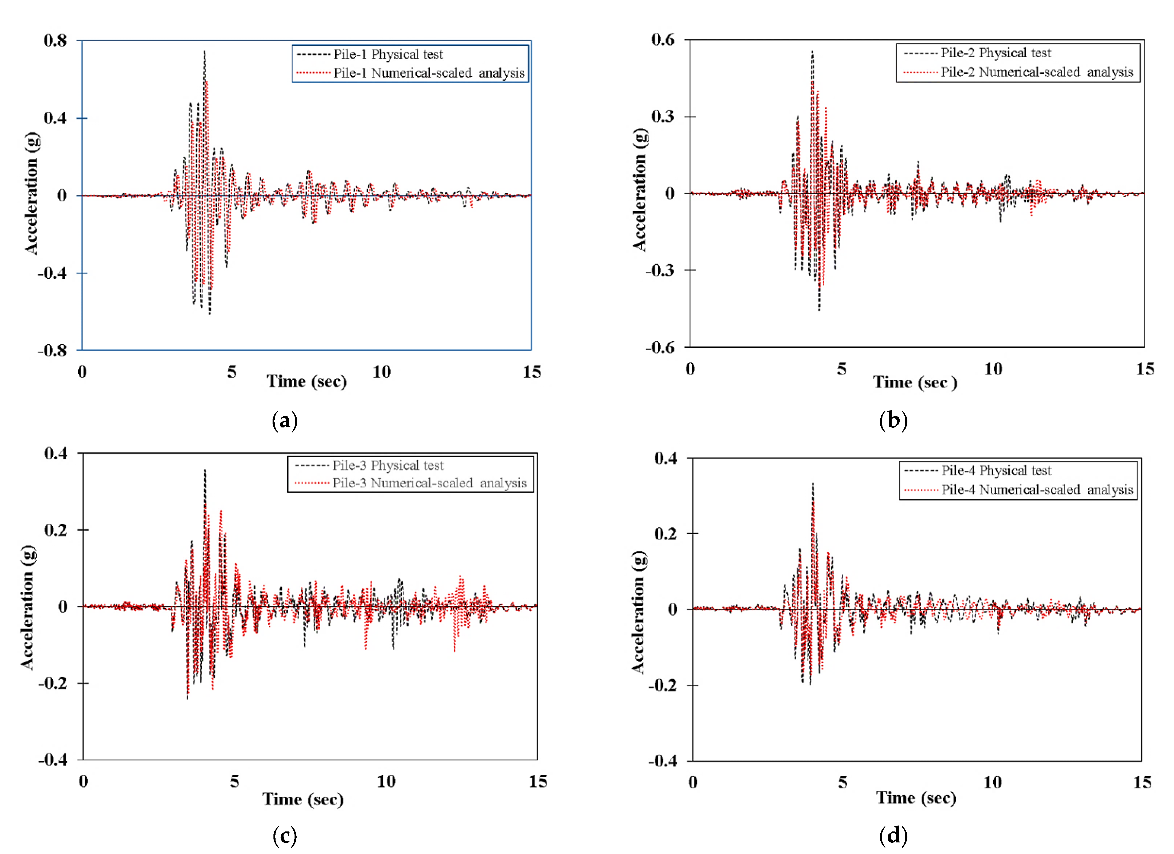
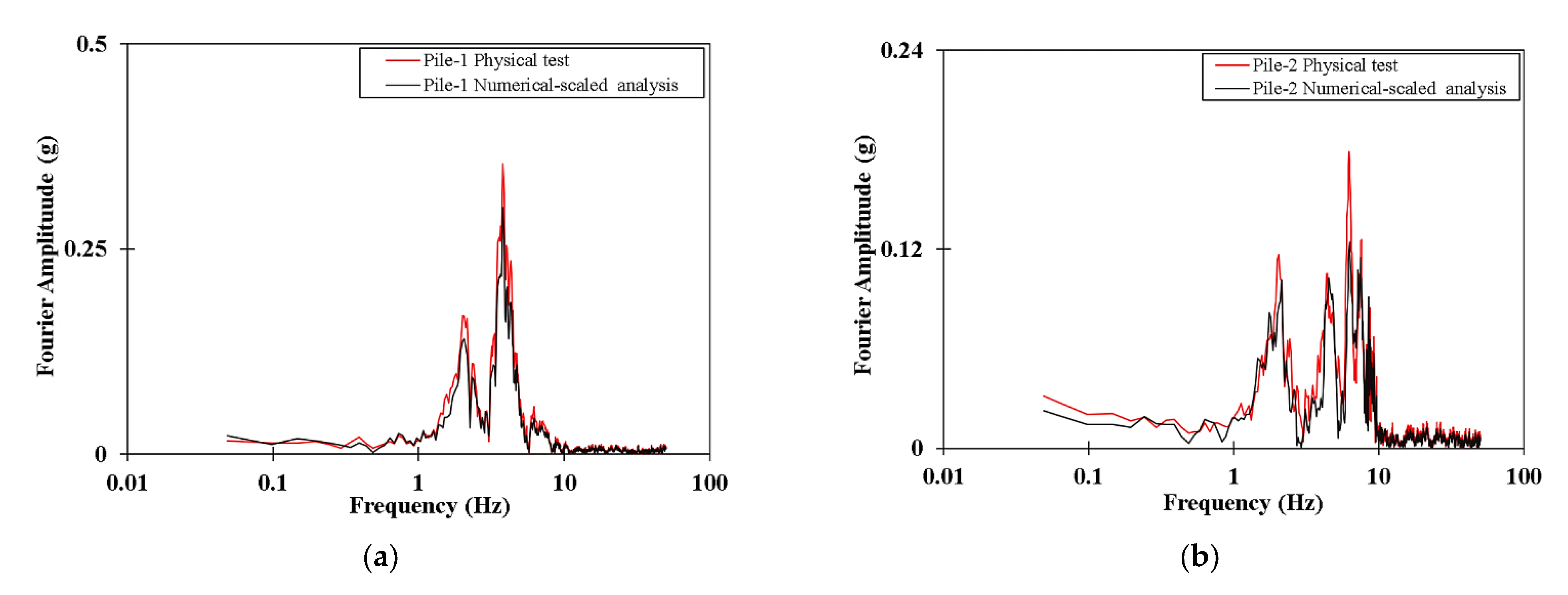
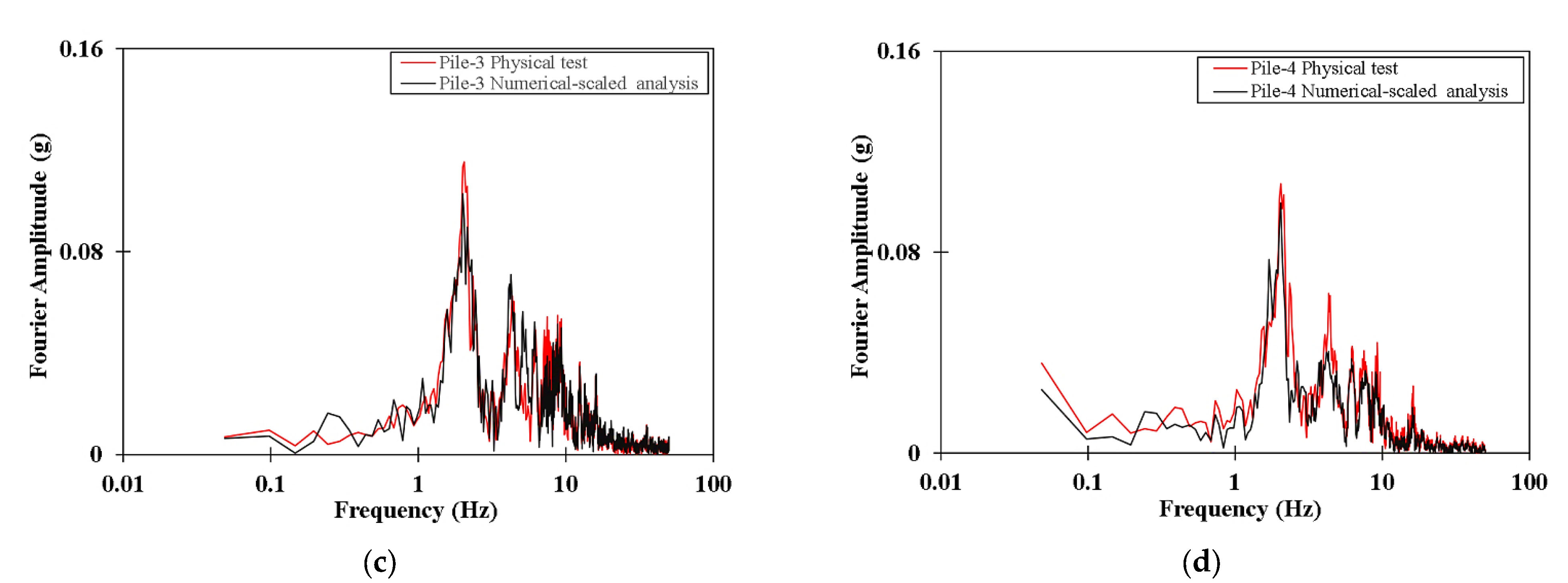
5.2. Validation of the Scaling Methodology

For piles that are designed to resist lateral loads, the ultimate and serviceability design limit states must be considered, including the potential load-displacement behaviour of a single pile. The potential load-displacement behaviour of a single pile is typically determined using either theoretical or/and semiempirical methods available in the literature. However, it is noteworthy that ignoring or simplifying the three-dimensional aspects of the lateral soil reaction and the variety of primary parameters governing the pile–soil interaction leads to less accurate predictions of the pile capacity. As mentioned earlier, full-scale tests are an excellent means for an accurate determination of small pile head deflections, but the expense and challenges of conducting these tests limits their practical value. Developing a scale model that represents the primary parameters of the prototype full-scale model is an efficient alternative. A number of problems in soil mechanics and structural analysis—primarily in the SSI area—can be studied using this validation approach. This method is a combination of two research areas, i.e., geotechnical and structural engineering, and is connected between the physical and numerical modelling programmes. The physical component is from the shaking table tests, which is then combined with the development of the 3D nonlinear FEA model to reflect the full and true behaviour of the system, including all interactions. The full-scale 3D numerical model is used to validate the inertial and kinematic behaviours of the scaled physical shaking table test.

In this context, the bending moment envelope, acceleration time history, acceleration Fourier amplitude, and acceleration response spectrum for the model are presented in Figure 16, Figure 17, Figure 18, Figure 19 and Figure 20, respectively. The results for these parameters were compared with the corresponding parameters used in the scaled physical shaking table test of the reference case study, [2] using the scale factors given in Table 2.

The bending moment parameter values of the full-scale numerical model were scaled down using a scaling factor equal to ${\lambda }^4$. Based on the procedure of validation described in Section 3, the resultant bending moment envelope behaviour of the scaled numerical model was compared to that from the reference case study. Figure 21 represents this validation. A similar process was conducted for the output acceleration time histories of the full-scale numerical model. As the test was performed in a 1g environment, the scaling factor corresponded to the acceleration parameter, which was taken as unity. In accordance with the data given in Table 2, the time parameter was required to be divided by a factor of ${\lambda }^{\frac{1}{2}}$. To create the other two parameters related to the acceleration time history behaviour; namely, the acceleration Fourier amplitude and acceleration response spectrum of the four cases of loading, the acceleration time history data were assessed using the SeismoSignal software [39]. Figure 22, Figure 23 and Figure 24 illustrate these comparisons for the four different types of pile head.

Pile behaviour under dynamic loading is substantially affected by the properties of the soil and pile, where pile properties represent pile material and shape properties. The nonlinear pile material modelling must be adopted to identify the pile lateral load capacity, associated bending moment, pile deflection, and pile material failure onset. The variation in the bending stiffness ($EI$) of a laterally loaded pile is a function of the bending moment distribution along the pile length and is represented as the moment–curvature relationship. As shown in Table 5 and Table 6, the target $EI$ of the model $(2.94 \mathrm{k}\mathrm{N}\mathrm{m}$, where the unit is derived from E per unit length equal to kN/m²/m and I is in m⁴) experienced an increase of 5.0% compared with the value of the computed scale model $(2.42 \mathrm{k}\mathrm{N}\mathrm{m}$). This deviation was reflected in the bending moment envelope values from the numerical simulation. Owing to the small difference in flexural rigidity values of the physical and numerical models, slight deviations in the corresponding bending moment envelopes can be observed in Figure 21, indicating that the current scaling and validation method could successfully examine and validate the inertial behaviour of the seismic SSI system when the primary parameters of the system were identified and scaled correctly.

The pile flexural stiffnesses along the deflected pile vary with the level of loading, pile material, moment–curvature relationship, and soil reaction, which influences the pile deflection pattern. Therefore, consistency among the primary dominated parameters of the distributions of pile deflection, bending moment, bending stiffness, and soil reaction must be maintained along with the pile. Nevertheless, based on the results presented in Figure 16, Figure 17, Figure 18, Figure 19 and Figure 20, it was shown that the scale model that was developed to predict the SSPSI response could represent all these primary parameters correctly. It permitted the evaluation of the soil–pile modulus based on the properties of the soil and pile, which included the pile flexural stiffnesses. The assessed model was thus influenced by the accuracy of the bending stiffness (in the model-to-prototype scaling) as well as the selected pile cross-section type and dimension. The proposed scaling and validation technique suggests that reducing the model flexural stiffness to simulate the correct prototype flexural stiffness may provide even more accurate results. However, considering a rational reduction factor is important and requires further research to provide reasonable guidelines.

In this scaling and validation technique, the static and/or dynamic pile response, including the pile head loads, deflections, and maximum moments, is considered on the basis of a constant bending stiffness ($EI$) along the pile length. Many studies revealed that the bending moment along the pile length did not significantly depend on the characteristics of the structure (e.g., [40]). Therefore, a small deviation between the numerical modelling according to prototype properties and the scaled physical test can be justified due to the 5% difference in $EI$ values. Moreover, the pile/soil compressibility ratio $K$ can be expressed as follows (see Equations (21)–(23)):

$$K=\frac{E_P}{E_s}$$

(21)

The lateral pile/soil stiffness ration $K_r$ is given as:

$$K_r=\frac{E_p I_p}{E_s D^4}$$

(22)

$K_r$ can be written as a function of $K$ as in the following equation:

$$K_r=\frac{ I_p}{ D^4} K$$

(23)

According to geotechnical codes such as AASHTO [41] and Eurocode 7, [42], the pile design phenomena depend mostly on the ultimate and serviceability limit states in which the load–deflection behaviour of the pile under lateral loads should be considered appropriately. The pile slenderness ratio and the pile–soil stiffness ratio are crucial factors that control the dynamic response of the pile–soil system. Realistic scaling and analysis of such these interactions should consider the nonlinear response of the system and the homogeneity of soil properties.

In pile design practice, the L/D ratio reflects the effect of the embedded length of the pile on the pile stiffness associated with the pile and the soil [43]. Increasing the L/D ratio results in an accumulative decline in the relative pile–soil stiffness $K_r$(Poulos and Davis 1980). These consequences are significantly influenced by the pile head conditions. The value of the degradation factor indicates that there is less reduction in the soil–pile interactive performance for arrangements with a relatively high L/D value. Low degradation factors induce a significant decline in the axial capacity of the pile due to the lower degradation factor values. For comparable dynamic loading properties and pile geometry parameters, a review of the literature shows that the degradation of the free headed pile is less significant compared to that of the fixed headed pile. The L/D ratio limitation must be identified carefully before starting the scaling process. Moreover, an accurate L/D ratio must be determined to produce the correct scale-model-to-prototype system behaviour associated with this significant scaling parameter.

The minimum wall thickness of the pile based on the D/t ratio is one of the principal parameters that must be considered to produce a scale model. According to Bala (2007), [44] the D/t ratio along the pile length must be small enough to prevent local buckling developing at stresses up to the yield strength of the pile material. The loading circumstances occur during the installation, so loading periods of the service life of the piling must be considered, and standard limitations of wall thickness t should be applied as a minimum requirement. Accordingly, the minimum pile wall thickness t should not be less than the value given in Equation (24):

$$t=6.35+\frac{D}{100}$$

(24)

where t and $D$are the wall thickness and diameter of pile in mm, respectively. This condition did not exist in the targeted and scale model properties. The minimum $t$ required is 6.8 $\mathrm{m}\mathrm{m}$, and the actual values of $t$ were 1.586 and 0.711 mm for the target and scale model, respectively. Depending on the class of soil type, pile buckling failure is associated with the D/t ratio; this is documented in the standard provisions [45], where the D/t ratios ranged between 15 and 45. In the current study, the difference between the D/t values of the target and scale models was significant, with a reduction of 76% between the target and the scale values. It was evident that the D/t value is a key factor in achieving an accurate similarity between the scale model and the prototype.

6. Conclusions

This paper presented and discussed a new and sophisticated approach to scaling and validating full-scale seismic soil–structure interaction problems using a careful and rational association between numerical and physical tests. This is a challenging issue with many unknown quantities, and establishing a reliable and accurate scaling procedure was difficult. The proposed methodology considers the scaling concept of implied prototypes as well as the “modelling of models” technique, which ensures a satisfactory level of model accuracy. Based on an extensive laboratory test that was previously conducted, a dimensional scaling factor λ equal to 8 was employed.

An advanced 3D finite element modelling using Abaqus software was also developed to further analyse the behaviour and proposed methodology. The characteristics, properties, and results of the physical shaking table test conducted by Meymand (1998) were adopted as the reference physical test. The data indicated a good correlation between the scaled numerical model results and those from the physical test when the scaling and validation method was used. The level of accuracy primarily depended on the level of scaling precision adopted, the selection of appropriate material properties to simulate the prototype materials, and the percentage difference between the target and computed values of the primary parameter of the system.

To stimulate the correct prototype flexural stiffness, the proposed scaling and validation technique indicates that the model flexural stiffness must be reduced by a reasonable reduction factor to achieve accurate results. Consideration of a rational reduction factor is a critical step that warrants further research to provide reasonable guidelines. According to the scaling law, the preparation of a clay specimen model was successfully defined for the physical and numerical tests. Therefore, this method of modelling can be adapted to other scale-modelling circumstances that require realistic soil behaviour, and it can validate the results using existing validation methods. Most seismic soil–pile–structure interaction models, such as the gap/slap mechanism, inertial forces of the superstructure, and kinematic soil–pile force, can be modelled correctly using the method developed and described herein.

References

1. Al Heib, M.; Emeriault, F.; Caudron, M.; Nghiem, L.; Heib, M.A.; Emeriault, F.; Caudron, M.; Nghiem, L.; Boramy, H. Large-scale soil-structure physical model (1g)—Assessment of structure damages. Int. J. Phys. Model. Geotech. 2014, 12, 138–152. [Google Scholar]
2. Meymand, P.J. Shaking Table Scale Model Tests of Nonlinear Soil-Pile-Superstructure Interaction in Soft Clay. 1998. Available online: http://nisee.berkeley.edu/meymand/files/intro.pdf (accessed on 15 July 2023).
3. Kline, S.J. Similitude and Approximation Theory; Springer: Berlin/Heidelberg, Germany; Stanford, CA, USA; New York, NY, USA; Tokyo, Japan, 1986. [Google Scholar]
4. Jonsson, D. Quantities, Dimensions and Dimensional Analysis. arXiv 2014, arXiv:1408.5024. Available online: http://arxiv.org/abs/1408.5024 (accessed on 15 July 2023).
5. Szϋcs, E. Similitude and Modelling; Elsevier Scientific Publishing Company: Amsterdam, The Netherlands, 1980; Volume 2. [Google Scholar]
6. Simitses, J. Structural Similitude and Scaling Laws for Laminated Beam-Plates; NASA: Washington, DC, USA, 1992. [Google Scholar]
7. Ramu, M.; Prabhu Raja, V.; Thyla, P.R. Establishment of structural similitude for elastic models and validation of scaling laws. KSCE J. Civ. Eng. 2013, 17, 139–144. [Google Scholar] [CrossRef]
8. Coutinho, C.P.; Baptista, A.J.; Dias Rodrigues, J. Reduced scale models based on similitude theory: A review up to 2015. Eng. Struct. 2016, 119, 81–94. [Google Scholar] [CrossRef]
9. Langhaar, H.L. Dimensional Analysis Theory Models, 13th ed.; Krieger Publishing Company: Malabar, FL, USA, 1980; ISBN 9780882756820. [Google Scholar]
10. Moncarz, P.; Krawinkler, H. Theory and Application of Experimental Model Analysis in Earthquake Engineering; The John A. Blume Earthquake Engineering Centre: Stanford, CA, USA, 2006. [Google Scholar]
11. Clough, R.W.; Pirtz, D. Earthquake Resistance of Rock-Fill Dams. J. Soil Mech. Found. Div. 1956, 82, 1–26. [Google Scholar] [CrossRef]
12. Seed, H.B.; Clough, R.W. Earthquake Resistance of Sloping Core Dams. J. Soil Mech. Found. Div. 1964, 90, 169–170. [Google Scholar] [CrossRef]
13. Candeias, P.X. Physical Modelling, Instrumentation and Testing; Seismic Engineering Research Infrastructures for European Synergies: Lisbon, Portugal, 2012. [Google Scholar]
14. Rocha, M. Similarity conditions in model studies of soil mechanics problems. In Proceedings of the Prepared to be Distributed to the Members of the 3rd International Conference on Soil Mechanics and Foundation Engineering, Zurich, Switzerland, 16–27 August 1953; Laboratorio Nacional de Engenharia Civil: Zurich, Switzerland, 1953. [Google Scholar]
15. Roscoe, K.H. Soils and model tests. J. Strain Anal. 1968, 3, 57–64. [Google Scholar] [CrossRef]
16. Kana, D.D.; Boyce, L.; Blaney, G.W. Development of a scale model for the dynamic interaction of a pile in clay. J. Energy Resour. Technol. Trans. ASME 1986, 108, 254–261. [Google Scholar] [CrossRef]
17. Iai, S. Similitude for Shaking Table Tests on Soil-Structure-Fluid Model in 1-g Gravitational Field. Soils Found. JSSMFE 1989, 29, 105–118. Available online: http://www.mendeley.com/research/geology-volcanic-history-eruptive-style-yakedake-volcano-group-central-japan/ (accessed on 15 July 2023).
18. Gohl, W.B. Response of Pile Foundations to Simulated Earthquake Loading: Expermental and Analytical Results. Ph.D. Thesis, University of British Columbia, Vancouver, BC, USA, 1991. [Google Scholar]
19. Scott, R.F. Centrifuge and modeling technology: A survey. Rev. Française Géotech. 1989, 48, 15–34. Available online: https://resolver.caltech.edu/CaltechAUTHORS:20140611-132033693 (accessed on 15 July 2023). [CrossRef] [Green Version]
20. Gibson, A. Physical Scale Modeling of Geotechnical Structures at One-G. Ph.D. Thesis, California Institute of Technology, Pasadena, CA, USA, 1997. [Google Scholar]
21. Al-Isawi, A.T.; Collins, P.E.F.; Cashell, K.A. Fully Non-Linear Numerical Simulation of a Shaking Table Test of Dynamic Soil-Pile-Structure Interactions in Soft Clay Using ABAQUS. Geotech. Spec. Publ. 2019, 2019, 252–265. [Google Scholar] [CrossRef] [Green Version]
22. Mylonakis, G.; Nikolaou, A.; Gazetas, G. Soil-pile-bridge seismic interaction: Kinematic and inertial effects. Part I: Soft soil. Earthq. Eng. Struct. Dyn. 1997, 26, 337–359. [Google Scholar] [CrossRef]
23. U.S. Geological Survey. PEER Ground Motion Database. Pacific Earthquake Engineering Research Centre. Available online: https://ngawest2.berkeley.edu/ (accessed on 15 July 2023).
24. Schellart, W.P.; Strak, V. A review of analogue modelling of geodynamic processes: Approaches, scaling, materials and quantification, with an application to subduction experiments. J. Geodyn. 2016, 100, 7–32. [Google Scholar] [CrossRef] [Green Version]
25. Harris, H.G.; Sabnis, G. Structural Modeling and Experimental Techniques; Taylor and Francis Group: Abingdon, UK, 1999. [Google Scholar]
26. Bonaparte, R.; Mitchell, J.K. The Properties of San Francisco Bay Mud at Hamilton Air Force Base, California; Department of Civil Engineering, University of California: Berkeley, CA, USA, 1979. [Google Scholar]
27. Dickenson, S.E. Dynamic Response of Soft and Deep Cohesive Soils during the Loma Prieta Earthquake of October 17, 1989; University of California: Berkeley, CA, USA, 1994. [Google Scholar]
28. Raoul, J.; Sedlacek, G.; Tsionis, G.; Raoul, J.; Sedlacek, G.; Tsionis, G. Eurocode 8: Seismic Design of Buildings Worked Examples; Publications Office of the European Union: Luxemborge, 2012. [Google Scholar]
29. Clough, R.W.; Penzien, J. Dynamics of Structures, 3rd ed.; CRC Press: London, UK, 2012; pp. 1–1019. [Google Scholar] [CrossRef]
30. Meymand, P.J.; Riemer, M.F.; Seed, R.B. Large scale shaking table tests of seismic soil-pile interaction in soft clay. In Proceedings of the 12th World Conference on Earthquake Engineering, Auckland, New Zealand, 30 January–4 February 2000; p. 2817. [Google Scholar]
31. Wang, S.T.; Reese, L.C. COM624P: Laterally Loaded Pile Analysis Program for the Microcomputer; Federal Highway Administration: Washington, DC, USA, 1993; p. 510. [Google Scholar]
32. Brittsan, D. Indicator Pile Test Program for the Seismic Retrofit of the East Approach Structure of the San Francisco-Oakland Bay Bridge; Foundation Testing and Implementation: Sacramento, CA, USA, 1995. [Google Scholar]
33. Langhaar, H. Dimensional Analysis and Theory of Models; John Wiley & Sons; Inc.: London, UK, 1951. [Google Scholar]
34. Smith, M. ABAQUS/Standard User’s Manual; Version 2018; SIMULIA: Providence, RI, USA, 2018; p. 1146. [Google Scholar]
35. Lucena, C.A.T.; Queiroz, P.C.O.; El Debs, A.L.H.C.; Mendonça, A.V. Dynamic Analysis of Buildings Using the Finite Element Method. In Proceedings of the 10th World Congress on Computational Mechanics, Sao Paolo, Brasil, 8–13 July 2012; pp. 4712–4726. [Google Scholar] [CrossRef] [Green Version]
36. Helwany, S. Applied Soil Mechanics with ABAQUS Applications; John Wiley & Sons; Inc.: Hoboken, NJ, USA, 2009; ISBN 978-0-471-79107-2. [Google Scholar]
37. Pitilakis, D.; Dietz, M.; Wood, D.M.; Clouteau, D.; Modaressi, A. Numerical simulation of dynamic soil-structure interaction in shaking table testing. Soil Dyn. Earthq. Eng. 2008, 28, 453–467. [Google Scholar] [CrossRef]
38. Alisawi, A.T.; Collins, P.E.F.; Cashell, K.A. Nonlinear numerical simulation of physical shaking table test, using three different soil constitutive models. Soil Dyn. Earthq. Eng. 2021, 143, 106617. [Google Scholar] [CrossRef]
39. SeismoSoft. Manual and program description of the program SeismoStruct. 2020. Available online: http://www.seismosoft.com (accessed on 15 July 2023).
40. Reese, L.C.; Wang, S.T. Analysis of Piles Under Lateral Loading with Nonlinear Flexural Rigidity. In Proceedings of the International Conference on Design and Construction of Deep Foundations, Orlando, FL, USA, 6–8 December 1994; pp. 842–856. [Google Scholar]
41. American Association of State Highway and Transportation Officials. AASHTO Provisional Standards 2021; American Association of State Highway and Transportation Officials: Washington, DC, USA, 2021. [Google Scholar]
42. Eurocode 7; Geotechnical design—Part 1: General Rules. British Standards Institution: London, UK, 2011; Volume 1.
43. Byrne, B.W.; McAdam, R.A.; Burd, H.J.; Beuckelaers, W.J.A.P.; Gavin, K.G.; Houlsby, G.T.; Igoe, D.J.P.; Jardine, R.J.; Martin, C.M.; Muir Wood, A.; et al. Monotonic laterally loaded pile testing in a stiff glacial clay till at Cowden. Géotechnique 2020, 70, 970–985. [Google Scholar] [CrossRef]
44. Bala, M. Recommended Practice for Planning, Designing and Constructing Fixed Offshore Platforms—Working Stress Design. Api Recomm. Pract. 2007, 2A–WSD, 242. [Google Scholar]
45. Hannigan, J.P.; Goble, G.G.; Thendean, G.; Likins, G.E.; Rausche, F. Design and Construction of Driven Pile Foundations. U.S. Dep. Transp. Fed. Highw. Adm. 1997, I. [Google Scholar]
Figure 1. Flowchart for forecasting the structural behaviour of full-scale prototypes using a physical test of a scale model.
Applsci 13 08626 g001
Figure 2. Constitutive behaviour of a scale model defined by stress and strain scaling factors. Modified from, Rocha (1958), [14].
Applsci 13 08626 g002
Figure 3. Critical state of soil with identical stress trajectories for prototype and model. Modified from Roscoe (1968), [15].
Applsci 13 08626 g003
Figure 4. Formulation of tangent modulus of the constitutive behaviour of scaled soil. modified from Iai (1989) [17].
Applsci 13 08626 g004
Figure 5. Definition of model soil properties utilising the steady-state line. Modified from Gibson (1997), [20].
Applsci 13 08626 g005
Figure 6. Full-scale container mounted on the shaking table with support struts and soil mixer/pump in the background; where: S1 = P-1, (Pile-1), S2 = P-2, (Pile-2), S3 = P-3, (Pile-3), S4 = P-4, (Pile-4), [2].
Applsci 13 08626 g006
Figure 7. Input motions including (a) acceleration for YBI90 and (b) acceleration response spectra for YBI90 [23].
Applsci 13 08626 g007
Figure 8. Flowchart of implied prototype-scaling methodology.
Applsci 13 08626 g008
Figure 9. Chart describing definitions and assumptions that affect the process of scale modelling that must be considered in the design of model components.
Applsci 13 08626 g009
Figure 10. Shear wave velocity versus (static) undrained shear strength of cohesive soils, the bule and red lines are the results boundaries, (after Dickenson 1994), [2].
Applsci 13 08626 g010
Figure 11. Lower- and upper-bound moment–curvature relationships for the prototype pile. * Aluminium tube dimensions were a diameter of 0.0508 m and a wall thickness of 0.00071 m.
Applsci 13 08626 g011
Figure 12. Theoretical and experimental moment–curvature relationships for dimensions of the aluminium tube model pile [2].
Applsci 13 08626 g012
Figure 13. Flowchart describing the validation methodology.
Applsci 13 08626 g013
Figure 14. Schematic of normal pressure and drag-force distribution [38].
Applsci 13 08626 g014
Figure 15. Images from the numerical simulation, including (a) a pile head mass of 72.7 kg, (b) a pile head mass of 45.36 kg, (c) a pile head mass of 11.40 kg, and (d) a pile head mass of 3.0 kg.
Applsci 13 08626 g015
Figure 16. Distribution of the acceleration response for full-scale numerical simulations of the shaking table, including those with a pile head mass of (a) 72.7 kg, (b) 45.36 kg, (c) 11.40 kg, and (d) 3.0 kg.
Applsci 13 08626 g016
Figure 17. Pile bending moment envelopes for arrangement with various pile head masses from the full-scale numerical model.
Applsci 13 08626 g017
Figure 18. Pile head acceleration time history responses from the full-scale numerical model of piles with pile head masses of (a) 72.7 kg, (b) 45.36 kg, (c) 11.40 kg, and (d) 3.0 kg.
Applsci 13 08626 g018
Figure 19. Fourier amplitude versus frequency (FFT) responses from the full-scale numerical model of piles with pile head masses of (a) 72.7 kg, (b) 45.36 kg, (c) 11.40 kg, and (d) 3.0 kg.
Applsci 13 08626 g019
Figure 20. Acceleration response spectra from the full-scale numerical model of piles with pile head masses of (a) 72.7 kg, (b) 45.36 kg, (c) 11.40 kg, and (d) 3.0 kg.
Applsci 13 08626 g020aApplsci 13 08626 g020b
Figure 21. Comparison of the pile bending moment envelopes for piles with various pile head masses from the full-scale numerical model and the scaled models.
Applsci 13 08626 g021
Figure 22. Comparison of the pile head acceleration time history responses from the physical test and the scaled numerical model for piles with pile head masses of (a) 72.7 kg, (b) 45.36 kg, (c) 11.40 kg, and (d) 3.0 kg.
Applsci 13 08626 g022
Figure 23. Comparison of the Fourier amplitude versus frequency (FFT) responses from the physical test and the scaled numerical model for piles with pile head masses of (a) 72.7 kg, (b) 45.36 kg, (c) 11.40 kg, and (d) 3.0 kg.
Applsci 13 08626 g023aApplsci 13 08626 g023b
Figure 24. Comparison of the acceleration response spectra from the physical test and the scaled numerical model for piles with pile head masses of (a) 72.7 kg, (b) 45.36 kg, (c) 11.40 kg, and (d) 3.0 kg.
Applsci 13 08626 g024