Abstract
Texas has abundant natural resources, making it a good place for renewable energy facilities to build. Unfortunately, property taxes are the highest tax on an incoming renewable energy facility in the state. In order to increase renewable energy in the state, Texas tax code Chapter 313 was introduced. Chapter 313 allows school districts the opportunity to offer a 10-year limit, ranging from USD 10 million to USD 100 million, on the taxable value of a new green energy project. With Chapter 313 ending in 2022, the following question is raised: how do tax incentives that increase the number of applications for producing renewable energy in Texas impact the wholesale, real-time pricing of electricity in the state? Skew-t regression models were implemented on a large dataset, focusing on the designated North, Houston, and West regions of the Electricity Reliability Council of Texas (ERCOT), since these regions account for 80% of the state’s energy consumption. Analysis focused on the hours ending at 3 AM, 11 AM, and 4 PM, due to the ERCOT’s time-of-day pricing. Three key findings related to the above question resulted. First, tax incentives that increase the number of active wind and solar facilities lead to a statistically significant (p < 0.0001) reduction in wholesale electricity price (USD/MWh), ranging between 2.31% and 6.6% across the ERCOT during different hours of the day. Second, for a 10% increase in tax-incentivized green energy generation, during a 24-hour period, there is a statistically significant (p < 0.0001) reduction in the generation cost (USD/MWh), ranging between 0.82% and 1.96%. Finally, electricity price reductions from solar energy are much lower than those from wind generation and/or are not statistically significant.
1. Introduction
Economic Dispatch is the implementation of electric generators based on the short-run marginal cost of production (e.g., generator fuel, variable operation, and maintenance expense). Prior to wholesale deregulation, electric utilities applied economic dispatch for their service territories. In some cases, utilities pooled generation resources to serve regional areas comprising several states (e.g., New England Power Pool). In Texas, economic dispatch is performed by the Electric Reliability Council of Texas (ERCOT). Among other things, the ERCOT ensures that wholesale energy supply requirements are attained through day-ahead and real-time markets in a least-cost fashion.
Since the early 2000s, in Texas, there has been a concerted effort to reduce the cost of electricity in an environmentally friendly way by stimulating the growth of renewable energy resources—wind and solar, in addition to baseload generation, namely nuclear energy. The costs of building renewable energy facilities are extremely high. But since these renewables rely only on wind or solar energy to generate electricity, their marginal costs of production depend only on maintenance and operation costs. Moreover, the Texas tax code chapter 313 also aimed at lowering capital or investment costs. Chapter 313 offers school districts the opportunity to provide even more benefits to businesses. It does so by offering a 10-year limit, ranging from USD 10m to USD 100m, on the taxable value of a new investment project in manufacturing or certain green energy projects [1].
Table 1 displays the cost of building renewable resources in the state of Texas. These are costs excluding battery storage. Adding a 60 MW/240-megawatt-hour (MWH) storage system to a 100 MW photovoltaic (PV) system costs between USD 171m and USD 173m [2]. The cost estimates in Table 1 refer only to capital investment, and not to fixed O&M expenses, that is, expenses incurred regardless of how much a resource is used. While investment costs for solar and wind facilities are high, fixed O&M expenses are relatively lower compared to those of nuclear plants.

Table 1.
Cost of building renewable resources in Texas.
The aims and contributions of this paper: A key principle underlying Economic Dispatch is the notion of the Merit-Order Effect (MOE), which ranks electricity generation from the lowest to the highest marginal cost of production: the lowest cost sources of generation are the first ones to be dispatched to meet demand. Thus, based on the MOE, increasing the supply of renewable energy resources during peak demand hours of the day, ceteris paribus, should result in lowering the wholesale price per MWh of electricity produced. The MOE metric is widely used in practice, and several researchers have studied its importance in the energy industry. Gelabert et al. (2011) quantified the MOE of renewable energy and cogeneration on electricity prices in Spain [5]. Sensfuß et al. (2008) provided a detailed analysis of the MOE on renewable electricity generation on spot market prices in Germany [6]. Cludius et al. (2014) found that the total MOE from wind generation resulted in a significant reduction in the price per MWh of electricity between 2008 and 2012 in Germany [7]. Sirin et al. (2020), using quantile regressions, quantified the MOE of variable renewable energy technologies in the Turkish electricity market [8]. Kang et al. (2022) used the MOE to construct hedging strategies, with the aim of minimizing risk due to volatilities in electricity prices [9]. Using quantile models, Rudolph et al. (2021) examined how the MOE varies with the level of wholesale electricity prices within the ERCOT [10].
Several researchers have also contributed to the literature on favorable governmental policies that have helped produce cleaner energy. These policies included low-cost financing, business-friendly tax policies, CO2 emission standards, carbon trading, interregional transmission connections, etc.; see: [11,12,13,14,15,16,17].
However, to the best of our knowledge, there has been no attempt to answer the following question: how do tax incentives that increase the active number of applications for producing renewable energy in the ERCOT impact the wholesale, real-time pricing of electricity in the state?
It should also be noted that none of the previous studies develop new variables with which to quantify tax incentivization and its subsequent impact on the MOE in the ERCOT. This research aims to fill this void by developing new variables, presented in Section 2. Section 3 implements skew-t regression models using our dataset. We note at the outset that the analytical aim of this paper is estimation, rather than prediction. Additionally, all of the regressions in this research are association models; hence, no causality is implied in any of the results. Section 4 provides a brief discussion and conclusion.
2. Data Details
The ERCOT uses a security-constrained economic dispatch model in order to set real-time wholesale energy prices. Conditional on demand, these prices are updated every 15 min in all of the ERCOT’s eight zones—North, Houston, West, South, Austin, San Antonio, Rayburn, and Lower Colorado River Authority. Each 15 min price serves as a datum for each of the dependent variables in this paper. Below, we describe that the sample size comprises 5844 points within each of the three zones. Hence, every regression model uses 5844 data points in order to estimate the regression parameters. Since almost 80% of the energy usage in Texas is concentrated in the North, Houston, and West regions, we focus on these regions in order to study the impact of tax policies on real-time pricing. Also, the models we employ are not time series regressions; hence, the time subscript is omitted throughout the remainder of the paper.
2.1. Dependent Variable: Price (USD/MWh)
We selected three hours in a 24 h cycle, as these are a fair representation of electricity usage and pricing. The hours we chose end at 3 AM, 11 AM, and 4 PM. Demand and price volatility tend to be the highest between 4 and 6 PM. The early morning hours have the least variability, and solar generation is absent after sunset. The 11 AM hour is more like the 4 PM hour, but not as variable.
Consider the summary statistics for the price variables in Table 2. Panels A through C of the table provide the price (USD/MWh) summaries for the hours ending at 3 AM, 11 AM, and 4 PM for North, Houston, and West regions, respectively. North and Houston are the largest energy-using zones in Texas. The West zone has the most wind-generating capacity. The mean and median prices in the three regions are generally comparable for the three hours. The volatility, as depicted by the standard deviation, is largest in West Texas, since this region depends primarily on wind generation. Other key differences are the skewness and kurtosis values across the zones for the three hours.
Table 2.
Summary statistics for price (USD/MWh).
These features of the price data are likely the result of differing energy demand levels across the three regions. It is important to understand the impact on prices resulting from large fluctuations in demand during peak and off-peak hours, even though it is difficult to pinpoint the exact reasons for some of these variations; seasonality plays a role. But another unique electricity pricing feature in the ERCOT must be considered in any statistical analysis of pricing data: wholesale price per MWh can be negative or close to zero, due to Locational Marginal Pricing (LMP).
LMP is a mechanism by which wholesale electricity prices quantify the value of electric power in different regions in the ERCOT, taking into consideration factors such as demand, generation, and the supply constraints inherent in the ERCOT’s state-wide transmission system. Theoretically and practically, LMP values can be negative. This happens when there is a surplus in generation. In such instances, certain resources—typically wind—are forced to curtail production. To remain economically viable, wind-generating plants are given a Production Tax Credit, which is paid in USD/MWh. In these instances, the real-time wholesale price of electricity will be negative, or almost zero.
For the above reasons, rather than using seasonal and/or LMP variables, we created dummy variables, based off the price data distributions shown in Table 2. These variables are critical to understanding how real-time prices are influenced by aberrant events or times within the dataset.
We also do not include lagged dependent variables, since the focus is on estimation, not prediction, in our real-time pricing regression models. Autoregressive and moving average variables are generally beneficial in time series regressions used for predictive analysis [18]. Such variables, typically, tend to increase predictive accuracy, but they also tend to dampen the effect sizes of other factors in the model, including outlier events captured via dummy variables, such as the LMP in energy models [19]. Damien et al. (2019) showed that autoregressive terms could prove useful in day-ahead ERCOT pricing models, where prices are set a day in advance of the supply of, and demand for, electricity the following day [20]. This is not the case in real-time pricing, where prices change every hour of the day, due to trading volatilities and other market-based demand and supply issues.
2.2. Independent Variables
The independent variables used in this paper are consistent with what other researchers have suggested and used in the present context [10,21,22]. The continuous independent variables (on the natural logarithm scale) include:
- Electricity demand (or load);
- Natural gas prices;
- Baseload nuclear power generation;
- Wind generation;
- Solar generation.
Coal prices are excluded, since coal is an inframarginal resource. That is, coal plants have operating costs which are typically lower than the market clearing price; hence, operating coal plants are insensitive to how market prices change. Natural gas generation is also excluded, since it is well-known that this data is highly collinear with load levels.
The dataset starts on 1 January 2015 and ends on 31 December 2018, and the data may be accessed at http://www.ercot.com/mktinfo. (URL accessed on 12 December 2022.)
Natural gas prices for Henry Hub (located in Erath, Louisiana) were obtained from the DOE/EIA.1. As Rudolph et al. (2021) note, Henry Hub prices replace local natural gas prices, since they bypass any endogeneity issue that local natural gas prices might induce [10]. Moreover, Henry Hub prices are highly correlated with local natural gas prices (r > 0.95). Daily natural gas prices are assumed constant across all 15 min intervals within each day.
Following Zarnikau et al. (2020), data for 2019 and early 2020 are omitted [23]. In 2019, the Public Utility Commission of Texas required the ERCOT to increase revenue to generators by shifting the Operating Reserves Demand Curve. Rudolph et al. (2021) noted that “the subsequent impact on market prices is very difficult to model” [10].
We also cannot incorporate the influence, if any, of climate change, on renewable energy and its subsequent impact on electricity pricing in Texas. We do not have the data, nor the modeling capabilities, to conduct such an analysis.
2.3. Dummy Variables for North and Houston Regions for Hours 3 AM, 11 AM, and 4 PM
From Table 2, for Hour 11 AM in the North region, the median price is USD 21.74. However, the minimum is only USD 0.07, while the maximum price is USD 556.92. In contrast, for the same region, during Hour 3 AM, the median, minimum, and maximum prices are USD 16.93, USD 0.01, and USD 82.7, respectively; note the dramatic reduction in the maximum value.
Consider Figure 1 Panels A, B, and C, which depict the time series of the price data for the North region at 11 AM, 4 PM, and 3 AM, respectively. The wild swings in prices are apparent in these three panels. Since energy demand tends to be higher at 11 AM and 4 PM than at 3 AM, we see much larger prices during the daytime. In contrast, prices tend to be generally lower at 3 AM. A careful examination of the data shows that some of the large values occur during the summer months, but not all of them.
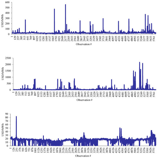
Figure 1.
Panel A (Top): Time series of North price, Hour 11 AM. Panel B (Middle): Time series of North price, Hour 4 PM. Panel C (Bottom): Time series of North price, Hour 3 AM.
We conducted a percentile analysis of the price data for Hours 11 AM and 4 PM in the North zone. For 11 AM, we chose a cutoff value of USD 50 at the upper tail of the data distribution, since only roughly 2% of the data are above USD 50. Similarly, for 4 PM, we choose a cutoff value of USD 90 at the upper tail. The analysis for the Hour 3 AM data yields cutoff values for the upper and lower ends of the price distribution, since the North price data at Hour 3 AM are left-skewed from Table 2. For the lower tail, we chose a cutoff value of USD 1.00, and for the upper tail we choose a cutoff value of USD 40. Collectively, these account for roughly 2.5% of the data.
The Houston region’s price data distribution behaves almost Identically to that of the North. Hence, the same dummy variable construction is used for the Houston price data distributions for the different hours. The above analysis yielded the following independent (dummy) variables for the North and Houston zones.
For Hours 11 AM and 4 PM in North and Houston:
If 11 am North Price >= $50, define NPrice50 = 1, else 0;
If 11 am Houston Price >= $50, define HPrice50 = 1, else 0;
If 4 pm North Price >= $90, define NPrice90 = 1, else 0;
If 4 pm Houston Price >= $90, define HPrice90 = 1, else 0.
For Hour 3 AM in North and Houston:
If 3 am North Price <= $1, define NPrice1 = 1, else 0;
If 3 am Houston Price <= $1, define HPrice1 = 1, else 0;
If 3 am North Price >= $40, define NPrice40 = 1, else 0;
If 3 am Houston Price >= $40, define HPrice40 = 1, else 0.
2.4. Dummy Variables for the West Region for Hours 3 AM, 11 AM, and 4 PM
We follow a similar process as above for the West region, working with Table 2 and Figure 2 Panels A, B and C. From Table 2, for Hour 11 AM in the West region, the median price is USD 21.68. The minimum is only USD 0.01, while the maximum price is USD 555.09. During Hour 3 AM, the median, minimum, and maximum prices are USD 16.93, USD 0.01 and USD 161.02, respectively.
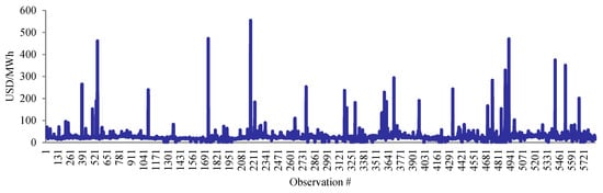
Figure 2.
Panel A (Top): Time series of West price, Hour 11 AM. Panel B (Middle): Time series of West price, Hour 4 PM. Panel C (Bottom): Time series of West price, Hour 3 AM.
Consider Figure 2 Panels A, B and C, which depict the time series of the price data for the West region at 11 AM, 4 PM, and 3 AM, respectively. Like in the North and Houston regions, dramatic swings in prices are apparent in these three plots. As noted previously, lagging prices at these time points will adversely impact the regression estimates of these event spikes on real-time pricing across the ERCOT.
Based on a percentile analysis of the price data for Hours 11 AM and 4 PM in the West zone, we chose a cutoff value of USD 50 at the upper tail, since only roughly 2% of the data are above USD 50.
A percentile analysis for the Hour 3 AM data yields cutoff values for the upper and lower tails of the price distribution. For the lower end, we chose a cutoff value of USD 1.00, and for the upper end, we choose a cutoff value of USD 32. Collectively, these account for roughly 2.5% of the data.
For Hours 11 AM and 4 PM in the West:
If 11 AM West Price >= $50, define WPrice50 = 1, else 0;
If 4 PM West Price >= $50, define WPrice50 = 1, else 0.
For Hour 3 AM in the West:
If West Price <= $1, define WPrice1 = 1, else 0;
If West Price >= $32, define WPrice32 = 1, else 0.
2.5. Defining New Tax Incentive Variables
From Texas Code Chapter 313, two new variables were created with which to analyze the effects that the chapter had on wholesale electricity prices in the ERCOT, stemming from renewable resources:
- The number of wind and solar applications;
- Total Gross Tax Savings (USD).
Data for these two variables came from the Texas Comptroller’s website (https://comptroller.texas.gov/economy/local/ch313/agreement-docs.php, accessed on 15 December 2022). The database is extensive and segmented by counties and regions. Data for the two variables were carefully constructed by first searching for each project application. The website also contains inactive applications, and often these are not clearly delineated. It is important to note that useful, tax-relevant data only come from active solar and wind applications. Hence, it is necessary to remove the inactive applications in the analysis; indeed, there are no tax savings data on inactive applications. Collating all of the pertinent information into a spreadsheet, we compiled the county/regional data into state-wide data. Even though the models in Section 3 will be at the regional level, the data on the two variables is too sparse, or non-existent, in all the regions. Additionally, real-time, wholesale pricing depends on the ERCOT level load, which is sometimes powered by transmitting renewable resources across regions. Therefore, it is practically relevant to consider the number of active wind and solar applications throughout the state.
Figure 3 and Figure 4 illustrate the number of active wind and solar applications and total gross tax savings from 2015 to 2018. Applications increase each year, starting with 16 in 2015 to 23 in 2018. Increases in active applications also increase the total gross tax savings per year. Information on the total gross tax savings is unavailable for the single solar application occurring in 2017, and is therefore absent from Figure 4. The absence of non-wind renewable resources will be borne out in the more rigorous statistical analyses in Section 3.
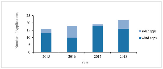
Figure 3.
Active wind and solar applications.
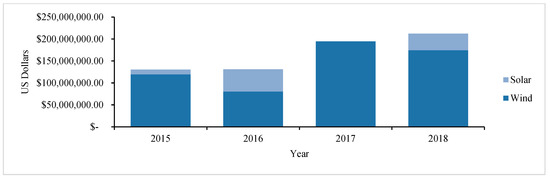
Figure 4.
Gross tax savings (USD).
Using the data corresponding to Figure 3 and Figure 4, and dropping the time (year) factor, one can construct a scatter plot to assess the relationship between applications and tax savings. Specifically, from Figure 4, it is evident that there is a noticeable jump in savings after 2016. Hence, we plot the total number of wind applications and the corresponding total savings over the four years. Consider Figure 5, which shows the scatter plot between wind applications and tax savings.
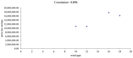
Figure 5.
Scatter plot of gross tax savings (USD) vs. wind applications.
The sizeable increase in gross tax savings when the number of wind applications increases from 12 to 16 is evident. The strong association (r = 0.896) between the two variables points to the possibility of using a dummy variable to model the marginal effect of wind applications on the wholesale electricity price in the ERCOT, instead of using the actual count of active wind applications. Indeed, based on the preceding discussion and the analysis in the next subsection, it is infeasible to use the discrete active wind application data in the regression models detailed in Section 3.
Additionally, going through a similar analysis for solar, we found a somewhat weak negative correlation (−0.357) between tax savings and solar applications. But, from a modeling perspective, one cannot ignore the effects of solar energy in Texas, since it is a growing renewable resource and is supported indirectly through PUCT Substantive Rule 25.173 (a)(1). Solar analysis is therefore included in conjunction with wind in subsequent chapters, despite recent data trends. To this end, consider Figure 6, which combines wind and solar applications, although wind applications dominate the number of solar applications in terms of gross tax savings. The correlation (0.882) between these variables is positive and large.
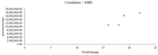
Figure 6.
Scatter plot of gross tax savings (USD) vs. wind and solar applications.
Based on Figure 6, we define a categorical (dummy) variable:
WSapp18 equals 1 if the number of wind and solar applications is at least 18, else 0.
This dummy variable will be used to capture the effect size of tax incentives on real-time electricity pricing. Note that this dummy variable indirectly links tax incentives to the number of active applications, since the latter may change for reasons other than tax incentives. But there is sufficient documentation in the database, which describes that most of the data for active applications are directly related to Chapter 313, namely tax savings. Also, from above, we see the strong, positive correlations between tax incentives and the number of applications. Hence, the dummy variable is an effective way of encapsulating the association between tax incentives and active applications.
2.6. Wind Generation vs. Active Wind Applications
To examine the importance of tax incentives on renewable resource electricity generation in ERCOT, one could pose the question: How much does each active wind application add to wind generation during different hours of the day? An answer to this question is possible by running a simple linear regression with the natural logarithm (LN) of wind generation at each hour serving as the dependent variable and the number of wind applications acting as the independent variable. However, such a regression analysis must be treated with some caution since the data on active wind applications is reported as a total in each year, whereas wind generation is obtained every 15 min.
The answer to the above question via a simple linear regression analysis may be a rough approximation; nonetheless, we ran a simple regression for Hours 3 AM, 11 AM, and 4 PM. Note that the following regression model does not change by region, since the number of wind applications and the wind generation data are for the ERCOT as a whole, rather than by region. For these reasons, and the others detailed previously, the WSapp18 variable is preferable to the actual count of wind and solar applications by region; WSapp18 will be used for the pricing models in Section 3.
With WGen denoting wind generation and Windapps denoting the number of active wind applications, the simple linear model for providing an answer to the above question is given through:
Regardless of region, for Hours 3 AM, 11 AM, and 4 PM, the values of slope b1 are estimated to be 0.0436, 0.051, and 0.055, respectively, with all p-values less than 0.0001. That is, each additional active wind application increases wind generation by 4.36%, 5.1%, and 5.5%, respectively, and the results are statistically significant.
Saving the rigorous pricing analysis for later, this preliminary conclusion offers some directional evidence to the main contention of this paper: tax incentives that increase the number of active wind applications statewide are associated with an increase in wind generation, which, in turn, could lead to a decrease in the wholesale price per MWh. Stated differently, the MOE from wind generation should contribute to more renewable energy over time, due to an increase in tax-incentivized wind generation.
In principle, one could execute a similar regression model for solar generation, as well. However, (a) the solar generation data are non-stationary; (b) the number of active solar applications is negligible; (c) the total contribution to the MOE from solar power is also negligible, based on the analysis later described in Section 3. For these reasons, the solar applications versus solar generation linear regression analysis, similar to the one above, is omitted.
3. Regression Analysis of Price (USD/MWh) Data for West, North, and Houston Regions in ERCOT
A common assumption in many statistical applications, including the current context, is that the error distribution in a linear regression model follows a normal distribution. But, for this assumption to hold, the data distribution has to be examined carefully; see Refs. [24,25]. The assumption of normality for the error distribution might be justified if the third and fourth moments—skewness and kurtosis—of the data distribution were approximately symmetric and exhibited low kurtosis. Additionally, the dataset should be free from multiple outliers. Skewness is a measure of symmetry, and kurtosis measures how the probability at the peak of the data distribution varies due to the thickness of the tails. For a standard normal distribution, the skew and kurtosis are zero and three, respectively. In a regression context, it is important to understand the properties of the data distribution, since inferences critically depend on them [26].
Based on our examination of the pricing data distributions (see Table 2), we use a natural log transformation of the pricing data, since they are highly asymmetric, with excessive kurtosis. Moreover, as shown in the previous section, due to the LMP feature in electricity pricing data, our dataset also has many outliers. In order to address these problems, in this section, we will assume that the error term has a skew-t distribution, instead of a normal distribution, for all of the pricing data regressions.
The use of skew-t distributions to model the error term in energy regression models and other contexts is well-documented; see, as examples, Refs. [9,19,27]. More generally, Azzalini and Genton (2008) state: “In a variety of practical cases, one reasonable option is to consider distributions which include parameters to regulate their skewness and kurtosis. As a specific representative of this approach, the skew-t distribution is explored in more detail and reasons are given to adopt this option as a sensible, general-purpose compromise between robustness and simplicity, both of treatment and of interpretation of the outcome” [28].
The univariate skew-t distribution, denoted ST (ξ, ω2, α, ν), is defined by introducing a multiplier to the Student-t density, which is a heavier-tailed distribution than the normal distribution. For a random variable x, the probability density function is given through:
where t (z; ν) is the density of a univariate Student-t distribution with degrees of freedom ν, and T (·; ν + 1) is the cumulative distribution function of a univariate Student-t distribution with ν + 1 degrees of freedom. The parameter ξ ∈ R regulates the location of the distribution, ω > 0 regulates the scale of the distribution, the shape parameter α ∈ R controls the asymmetry of the distribution, and the degrees-of-freedom parameter ν > 0 controls the tails of the distribution. When α = 0, the density in Equation (1) reduces to the standard Student-t density. When α = 0, and as ν tends to ∞, the skew-t density reduces toward the normal density. By introducing an extra parameter for regulating the tails, the skew-t distribution accommodates outlying observations.
Thus, the skew-t distribution explicitly allows for varying levels of asymmetry and kurtosis in the data distributions, while also coping with outliers. All three of these features are prevalent in the pricing data we use in this research. Hence, the skew-t distribution will prove useful in estimating the regression coefficients.
We construct regression models for the hours ending at 3 AM, 11 AM, and 4 PM within each of the three regions—West, North and Houston. A total of 18 regression models are used in order to study the relationships between the various independent variables described previously and the price data. Of the 18 models, 9 correspond to the analysis using skew-t error distributions, and 9 correspond to the analysis using the normal distribution. The latter was conducted mainly for comparison purposes, in order to illustrate any differences in the overall inferences if one assumed a symmetric distribution to model the regression error term for asymmetric price data.
In the following subsections, as noted previously, the dependent and all of the continuous independent variables are on the natural logarithm scale. Thus, the corresponding regression coefficients are all elasticities, facilitating easy interpretation of the analytical results in terms of percent changes.
Recall that the price data are observed every 15 min. But our regressions are not time series models; hence, we do not use any time subscript for the price variable. It suffices to note that each regression is estimated using 5844 data points. Additionally, as described previously, we do not use autoregressive/moving average variables in the analysis; these variables could prove useful if we were predicting the price every 15 min. But our paper does not deal with predictions: its focus is on estimating contemporaneous marginal effects.
3.1. Hourly Models for West Region Price Data
Hour 3 AM Model:
Hour 11 AM Model:
Hour 4 PM Model:
Variable Definitions:
For convenience, the dummy variable definitions from above follow:
- WSapp18: Active wind and solar applications equaling 18 or more is coded 1, else 0;
- Wprice1: In the 3 AM model, if price is at most USD 1, Wprice1 is coded 1, else 0;
- Wprice32: In the 3 AM model, if price is at least USD 32, Wprice32 is coded 1, else 0;
- Wprice50: In the 11 AM model, if price is at least USD 50, Wprice50 is coded 1, else 0;
- Wprice90: In the 4 PM model, if price is at least USD 90, Wprice90 is coded 1, else 0;
- NGprice: Natural Gas Price;
- Wgen: Wind Generation;
- Ngen: Nuclear Generation;
- Wload: West Load;
- REload: Rest of ERCOT Load is always defined as the ERCOT Load minus the specific region’s load; hence, here it is the ERCOT Load minus West Load, and similarly for the other regions in the models in Section 3.3 and Section 3.4.
3.2. Analysis of Hourly Models for West Region Price Data
Recall the following from Section 2: Could incentivizing renewable resource electricity generation via tax policies, such as Texas Code Chapter 313, lead to reductions in the cost of electricity in the real-time, wholesale energy market in the ERCOT? That is, is there an association between tax-incentivized power generation and wholesale prices in the energy market?
Additionally, from the perspective of economic dispatch, increased electricity demand throughout the ERCOT is first met by those resources that are the cheapest to generate and deliver to the grid—the renewable resources, wind and solar. From a pricing perspective, the merit-order effect (MOE) of this dispatching protocol should contribute toward lowering real-time wholesale electricity prices throughout the state. The parameter estimates of the nuclear, wind, and solar generation variables will quantify the MOE.
The following empirical analyses will address the above salient points, in addition to other insights. Using STATA, under the assumption of normally distributed errors, the regression parameters were estimated using least squares. Under the assumption that the errors follow a skew-t distribution, the regression parameters are maximum likelihood estimates, which were obtained iteratively.
Refer to Table 3 and focus on the Hour 3 AM skew-t regression estimates for the West region. All the regressor variables are statistically significant (p < 0.0001, and coefficient signs are as expected). The standard errors are given in parentheses.
Table 3.
West region skew-t regression estimates.
- WSapp18: The focus of this research is to study the impact of tax policies on the wholesale price of electricity. Let us begin by considering the marginal effect of the variable WSapp18, whose coefficient estimate equals −0.0492. When the number of active wind and solar applications is at least 18, the price per MWh declines by about 5% (=e0.0492) at 3 AM in the West region, which is a statistically significant reduction in price. Note that, even though there is no solar generation at 3 AM, it may be possible to produce and store solar energy, which could then be used if demand was high.
- MOE: Of interest here is the merit-order effect (MOE) of nuclear and wind generation. Each 1% increase in nuclear generation, namely LN(Ngen), is associated with a 0.11% drop in price per MWh. A 1% increase in wind generation (LN(Wgen)) is associated with a 0.0851% reduction in price per MWh. Hence, a 10% increase in either energy source will lead to roughly 1.107% (=1.100.1119) and 0.81% (=1.100.0851) reductions in price per MWh, respectively. Coupled with the marginal effect of WSapp18, we can conclude that a tax policy aimed at incentivizing the number of active wind and solar applications is associated with declines in the wholesale price of electricity, ceteris paribus, since it will increase wind and solar generation—the less expensive renewable resources.
Price Dummies: Next, consider the impact of extremely small and large prices in the price data distribution (see Table 2 in Section 2 for the minimum and maximum summary statistics). From Table 3, for the variable Wprice1, when prices are at most USD 1, there is a roughly 1493% decline in price, compared to when prices are greater than USD 1. This drastic reduction in price is likely induced by the LMP. Recall from Section 2 that LMP is a wholesale electricity price construct that quantifies the value of electric power at different regions in the ERCOT, taking into consideration factors such as demand, generation, and the supply constraints inherent in the ERCOT’s state-wide transmission system. Theoretically and practically, LMP values can turn negative. This happens when there is a surplus of generation that cannot be delivered outside of its zone due to transmission constraints. In such instances, the prices of certain resources, typically wind, are forced down to curtail generation.
- For the variable Wprice32, when prices are at least USD 32, real-time prices in the West region increase by about 380%, compared to when prices are below USD 32. In this regard, recall the summary statistics of the price distributions from Section 2. The median and mean prices at 3 AM in the West region are USD 16.93 and USD 17.16, respectively. The minimum and maximum prices are USD 0.01 and USD 161.02. Indeed, a percentile analysis revealed that roughly 5% of the prices are extreme at both tails of the price distribution. As described previously, extreme prices could be the result of seasonality and/or the LMP effect. Lower prices are typically the result of low demand, as at 3 AM. On the other hand, when demand and prices are high, if the MOE from renewable resource generation is sizeable, that would dampen the price, since the cost of delivering energy to the grid will decline. It is clear from the above parameter estimates discussion of the MOE that more gains from wind generation could be had, if the number of active wind farms were to grow in Texas.
- Natural Gas Price: The coefficient estimate for LN(NGprice) is 0.5133 (p < 0.0001). For a 1% increase in natural gas price, the wholesale electricity price increases by 0.5133%.
- West Load: The coefficient estimate for LN(Wload) is 0.2544 (p < 0.0001). For a 1% increase in demand in the West, the wholesale electricity price in the West at 3 AM increases by 0.2544%.
- Rest of ERCOT Load: The coefficient estimate for LN(REload) is 0.1273 (p < 0.0001). For a 1% increase in demand in the rest of the ERCOT, the wholesale electricity price in the West at 3 AM increases by 0.1273%.
- Normal Regression Comparison: Finally, consider the normal regression parameter estimates in Table 4. When compared to the skew-t estimates, a most striking feature here is that the WSapp18 variable is not significant, and its marginal effect is almost zero. A second counterintuitive conclusion is that the impact of demand in the West (Ln(Wload)) is not significant. A third key difference is that the standard errors under the normal regression model tend to be higher than those from the skew-t model. This is because the standard error (i.e., the standard deviation of the estimated errors) in the normal regression fails to account for the asymmetry, kurtosis, and outliers in the data distribution. Thus, these regression results validate the importance of using a skew-t distribution for the error term in the regression to better account for idiosyncrasies in the data distributions.
Table 4. West region normal regression estimates.
Next, consider Table 3 and focus on the Hour 11 AM estimates. All of the regressor variables are statistically significant (p < 0.0001), and the coefficient signs are as expected. We focus on the most important variables here, since the inferences for the others are similar to those from the 3 am description, given above.
- WSapp18: The WSapp18 variable’s regression coefficient equals −0.066. When the number of active wind and solar applications is at least 18, the wholesale price per MWh declines by about 6.6%. This further confirms the importance of tax policies on the pricing of electricity in the ERCOT market—the larger the number of active wind and solar applications, the greater the reduction in the wholesale price, since electricity from these resources will be dispatched first.
- MOE: The marginal effects of nuclear, wind, and solar generation are −0.1118%, −0.1032%, and −0.107%, respectively. Nuclear generation is more expensive than wind and solar generation. That means, from an MOE perspective, that the latter resources will be dispatched first. Hence, if more electricity is generated from these renewable resources, vis-à-vis a larger number of wind and solar applications, eventually, the overall contribution from renewables to the ERCOT’s grid might exceed that of nuclear power.
- Normal Regression Comparison: Finally, in the normal regression model, once again, the parameter estimates are different than the ones from the skew-t model, as shown in Table 4. A most noteworthy conclusion is that the solar generation variable (Sgen) is not significant, unlike in the skew-t model.
Now, consider Table 3 and focus on the Hour 4 PM estimates. All of the regressor variables are statistically significant (p < 0.0001), and the coefficient signs are as expected, except for that of solar generation (Sgen). This is not surprising, since, as discussed in Section 2, solar power is still a very small component of overall renewable energy resources in Texas. The time series data for solar energy are non-stationary; hence, the signs of the estimates can vary from their expectations. Inferences from the WSapp18 and MOE variables are similar to the ones detailed under hours 3 AM and 11 AM, above.
3.3. Hourly Models for North Region Price Data
The regression equations are similar to those for the West region. Almost all of the variable definitions are identical to those for the West models. For the North model, the new variables are as follows:
- Nprice40: in the 3 AM model, if price is at least USD 40, Nprice40 is coded 1, else 0;
- Nprice90: in the 4 PM model, if price is at least USD 90, Nprice90 is coded 1, else 0;
- Nload: North Load.
3.4. Hourly Models for Houston Region Price Data
Again, the regression equations are similar to those for the West region. For the Houston model, the new variables are as follows:
- Hprice40: in the 3 AM model, if price is at least USD 40, Hprice40 is coded 1, else 0;
- Hprice90: in the 4 PM model, if price is at least USD 90, Hprice90 is coded 1, else 0;
- Hload: Houston Load.
3.5. Analysis of Hourly Models for North and Houston Price Data
Since the inferences for the North and Houston regions are almost identical, we treat them together. Consider Table 5 and Table 6, which correspond to the parameter estimates for the North and Houston regions, respectively.
Table 5.
North region skew-t estimates.
Table 6.
Houston region skew-t estimates.
- WSapp18 at 4 PM: The WSapps18 variable results in a significant reduction in price per MWh in both regions—6.2% in the North, and 5.4% in Houston.
- MOE at 4 pm: Solar generation (Sgen) is significant, but positive, in both regions. Importantly, these marginal solar effects are negligible. The conflicting positive coefficient sign is once again the result of very little solar energy in the ERCOT grid at 4 PM, when compared to the energy present from nuclear and wind sources. This is yet another reason we chose to combine wind and solar active applications in the models. Over time, it may become viable to separate solar and wind applications in the modeling process. The nuclear generation coefficient estimates for the North and Houston regions are −0.1188% and −0.1967%, and for wind generation, the estimates are −0.0931% and −0.0717%, respectively.
- WSapp18 at 11 AM: The WSapps18 variable results in a statistically significant (p < 0.0001) reduction in price per MWh in both regions—3.80% in the North, and 3.95% in Houston.
- MOE at 11 AM: Solar generation (Sgen) is significant in both regions, but the marginal effects are almost zero. This is not surprising, since, as noted before, solar energy is still in its infancy in the ERCOT. The nuclear generation coefficient estimates for the North and Houston regions are −0.1124% and −0.1695%, and for wind generation, the estimates are −0.0917% and −0.0666%, respectively, with p < 0.0001.
- WSapp18 at 3 AM: The WSapps18 variable results in a statistically significant (p < 0.0001) reduction in price per MWh in both regions—2.31% in the North, and 3.1% in Houston.
- MOE at 3 AM: The nuclear generation coefficient estimates for the North and Houston regions are −0.1592% and −0.1760%, and for wind generation, the estimates are −0.0965% and −0.0824%, respectively, with p < 0.0001.
- Finally, the price dummies, natural gas price, North load, Houston load, and rest of the ERCOT load, in the North and Houston regions are generally consistent with the inferences described above for the West region. Likewise, the normal regression analyses are similar to that for the West region, and is thus omitted in this paper.
In summary, based on the regression analyses of the three regions, this paper empirically validates the conjecture that offering tax incentives to increase the number of active wind and solar applications is associated with meaningful reductions in the wholesale price of electricity in the ERCOT. As seen above, this has implications for the MOE, since, in terms of economic dispatch, less expensive renewable energy can be passed on to the final consumer of electricity in the form of lower prices, especially when the demand for electricity increases.
4. Discussion and Conclusions
In this paper, we hypothesized that the real-time wholesale price of electricity (USD/MWh) in the ERCOT decreases in response to the number of active wind and solar applications; i.e., there is an association between the number of active wind and solar applications and the price of electricity in the ERCOT. Increased electricity demand throughout the ERCOT is first met by resources that are the cheapest to produce and deliver to the grid—the renewable resources, wind and solar. Hence, from a pricing perspective, the merit-order effect (MOE) of this dispatching protocol should contribute toward lowering real-time wholesale electricity prices throughout the state.
Three key inferences resulted from our analysis. First, tax incentives that increase the number of active wind and solar facilities lead to a statistically significant (p < 0.0001) reduction in wholesale electricity price (USD/MWh), ranging between 2.31% and 6.6% across the ERCOT during different hours of the day. Second, for a 10% increase in tax- incentivized green energy generation during a 24 h period, there is a statistically significant (p < 0.0001) reduction in the production cost (USD/MWh), ranging between 0.82% and 1.96%. Finally, electricity price reductions from solar energy are much lower than those from wind generation and/or are not statistically significant.
As the electricity market in Texas attempts to increase its dependence on green energy via friendly tax policies for the producers of renewable resources, the MOE of these resources will increase, thereby reducing real-time wholesale prices.
While the statistical association between wind generation and wholesale pricing is unambiguous, the same is not true of solar generation. Complementing previous research, such as Maciejowska (2020) and Rudolph et al. (2021), we find that, even with increased tax incentives, the MOE from solar energy is either negligible, or is not statistically significant [10,29]. As described in previous sections, solar energy is still a growing resource in the ERCOT. The US Energy Information Administration (EIA) estimated that, between 2016 and 2017, the net solar generation in Texas rose from 96,000 MWh to 199,000 MWh, which only accounts for about 1.35% of the state’s electricity needs. However, the EIA projects that, by 2040, solar capacity in Texas could increase to 4 GW, making it the largest producer of solar energy nationwide.
According to the Texas Comptroller’s Office, “Texas is experiencing a population boom, adding nearly 4 million residents over the past decade”. The EIA estimates that the influx of new companies and migrating populations will increase the demand for electricity by at least 25% by 2035. (https://www.eia.gov/outlooks/aeo/pdf/0383(2011).pdf, accessed on 15 December 2022).
Paired with our results, this rapid demand growth for energy raises interesting questions for future research. How much and what type of tax incentives are needed in order to increase wind and solar energy to meet the demand for energy in Texas? And, if green energy lowers wholesale electricity prices too much, how would that affect the profitability of producing renewable resources? The answers to these questions will be pursued in subsequent research.
Author Contributions
Both authors contributed equally to all aspects of this paper. All authors have read and agreed to the published version of the manuscript.
Funding
This research received no external funding.
Institutional Review Board Statement
Not applicable.
Informed Consent Statement
Not applicable.
Data Availability Statement
Not applicable.
Conflicts of Interest
The authors declare no conflict of interest.
References
- Texas Taxpayers and Research Association. School property tax limitations and the impact on state finance. TTARA 2021, 1–16. Available online: www.ttara.org (accessed on 10 December 2022).
- Feldman, D.; Ramasamy, V.; Fu, R.; Ramdas, A.; Desai, J.; Margolis, R. U.S. Solar Photovoltaic System and Energy Storage Cost Benchmark: Q1 2020; National Renewable Energy Laboratory: Golden, CO, USA, 2020.
- Feldman, D.; Robert, M. NREL: Fall 2021 Solar Industry Update; National Renewable Energy Laboratory: Golden, CO, USA, 2021.
- Walker, A.; Lockhart, E.; Desai, J.; Ardani, K.; Klise, G.; Lavrova, O.; Tnasy, T.; Deot, J.; Fox, B.; Pochiraju, A. Model of Operation-and Maintenance Costs for Photovoltaic Systems; National Renewable Energy Laboratory: Golden, CO, USA, 2020. Available online: https://www.nrel.gov/docs/fy20osti/74840.pdf (accessed on 10 December 2022).
- Gelabert, L.; Labandeira, X.; Linares, P. An ex-post analysis of the effect of renewable and cogeneration on Spanish electricity prices. Energy Econ. 2011, 22, 559–565. [Google Scholar] [CrossRef]
- Sensfuß, F.; Ragwitz, M.; Genoese, M. The merit-order effect: A detailed analysis of the price effect of renewable electricity generation on spot market prices in Germany. Energy Policy 2008, 36, 3086–3094. [Google Scholar] [CrossRef]
- Cludius, J.; Hermann, H.; Matthes, F.; Graichen, V. The merit-order effect of wind and photovoltaic electricity generation in Germany 2008–2016: Estimation and Distributional Implications. Energy Econ. 2014, 44, 302–313. [Google Scholar] [CrossRef]
- Sirin, S.M.; Yilmaz, B.N. Variable renewable energy technologies in the Turkish electricity market: Quantile regression analysis of the merit-order effect. Energy Policy 2020, 144, 111660. [Google Scholar] [CrossRef]
- Kang, L.; Walker, S.; Damien, P.; Bunn, D. Bayesian estimation of electricity price risk with a multifactor mixture of densities. Quant. Financ. 2022, 22, 1535–1544. [Google Scholar] [CrossRef]
- Rudolph, M.; Damien, P.; Zarnikau, J. An empirical study of the merit-order effects in the Texas energy market via quantile regression. Int. J. Adv. Oper. Res. 2021, 13, 258–274. [Google Scholar] [CrossRef]
- Alagappan, L.; Orans, R.; Woo, C.K. What drives renewable energy development? Energy Policy 2011, 39, 5099–5104. [Google Scholar] [CrossRef]
- Zarnikau, J. Successful renewable energy development in a competitive electricity market: A Texas case study. Energy Policy 2011, 39, 3906–3913. [Google Scholar] [CrossRef]
- Lam, J.C.K.; Woo, C.K.; Kahrl, F.; Yu, W.K. What moves wind energy development in China? Show me the money! Appl. Energy 2013, 105, 423–429. [Google Scholar] [CrossRef]
- Woo, C.K.; Olson, A.; Chen, Y.; Moore, J.; Schlag, N.; Ong, A.; Ho, T. Does California’s CO2 price affect wholesale electricity prices in the western U.S.A.? Energy Policy 2017, 110, 9–19. [Google Scholar] [CrossRef]
- Woo, C.K.; Chen, Y.; Olson, A.; Moore, J.; Schlag, N.; Ong, A.; Ho, T. Electricity price behavior and carbon trading: New evidence from California. Appl. Energy 2017, 204, 531–543. [Google Scholar] [CrossRef]
- Woo, C.K.; Chen, Y.; Zarnikau, J.; Olson, A.; Moore, J.; Ho, T. Carbon trading’s impact on California’s real-time electricity market prices. Energy 2018, 159, 579–587. [Google Scholar] [CrossRef]
- Woo, C.K.; Zarnikau, J. Renewable energy’s vanishing premium in Texas’s retail electricity pricing plans. Energy Policy 2019, 132, 764–770. [Google Scholar] [CrossRef]
- Box, G.E.P.; Jenkins, G.M.; Reinsel, G.C. Time Series Analysis: Forecasting and Control, 4th ed.; Wiley: Hoboken, NJ, USA, 2008. [Google Scholar]
- Gianfreda, A.; Bunn, D. A stochastic latent moment model for electricity price formation. Oper. Res. 2018, 66, 1189–1203. [Google Scholar] [CrossRef]
- Damien, P.; Fuentes-Garcia, R.; Mena, R.; Zarnikau, J. Impacts of day-ahead versus real-time market prices on wholesale electricity demand in Texas. Energy Econ. 2019, 81, 259–272. [Google Scholar] [CrossRef]
- Zarnikau, J.; Woo, C.K.; Zhu, S.S. Zonal merit-order effects of wind generation development on day-ahead and real-time electricity market prices in Texas. J. Energy Mark. 2016, 9, 17–47. [Google Scholar] [CrossRef]
- Tsai, C.H.; Eryilmaz, D. Effect of wind generation on ERCOT nodal prices. Energy Econ. 2018, 76, 21–33. [Google Scholar] [CrossRef]
- Zarnikau, J.; Woo, C.K.; Zhu, S.S.; Tsai, C.H. Will Texas’s operating reserve demand curve likely provide adequate investment incentive for natural-gas-fired generation? Energy Policy 2020, 137, 111143. [Google Scholar] [CrossRef]
- DeGroot, M.; Schervish, M. Probability and Statistics, 4th ed.; Pearson Publication: London, UK, 2018. [Google Scholar]
- Kang, L.; Damien, P.; Walker, S. On a transform for modeling skewness. Braz. J. Probab. Stat. 2021, 35, 335–350. [Google Scholar] [CrossRef]
- Hill, C.R.; Griffiths, W.E.; Lim, G.C. Principles of Econometrics, 5th ed.; Wiley Publications: Hoboken, NJ, USA, 2018. [Google Scholar]
- Abramova, E.; Bunn, D. Forecasting the intra-day spread densities of electricity prices. Energies 2020, 13, 687. [Google Scholar] [CrossRef]
- Azzalini, A.; Genton, M.G. Robust likelihood methods based on the skew-t and related distributions. Int. Stat. Rev. 2008, 76, 106–129. [Google Scholar] [CrossRef]
- Maciejowska, K. Assessing the impact of renewable energy sources on the electricity price level and variability—A quantile regression approach. Energy Policy 2020, 85, 104532. [Google Scholar] [CrossRef]


Disclaimer/Publisher’s Note: The statements, opinions and data contained in all publications are solely those of the individual author(s) and contributor(s) and not of MDPI and/or the editor(s). MDPI and/or the editor(s) disclaim responsibility for any injury to people or property resulting from any ideas, methods, instructions or products referred to in the content. |
© 2023 by the authors. Licensee MDPI, Basel, Switzerland. This article is an open access article distributed under the terms and conditions of the Creative Commons Attribution (CC BY) license (https://creativecommons.org/licenses/by/4.0/).