Prediction of Internal Temperature in Greenhouses Using the Supervised Learning Techniques: Linear and Support Vector Regressions

Abstract

Agricultural greenhouses must accurately predict environmental factors to ensure optimal crop growth and energy management efficiency. However, the existing predictors have limitations when dealing with dynamic, non-linear, and massive temporal data. This study proposes four supervised learning techniques focused on linear regression (LR) and Support Vector Regression (SVR) to predict the internal temperature of a greenhouse. A meteorological station is installed in the greenhouse to collect internal data (temperature, humidity, and dew point) and external data (temperature, humidity, and solar radiation). The data comprises a one year, and is divided into seasons for better analysis and modeling of the internal temperature. The study involves sixteen experiments corresponding to the four models and the four seasons and evaluating the models’ performance using R${}^2$, RMSE, MAE, and MAPE metrics, considering an acceptability interval of ±2 ${}^{°}$C. The results show that LR models had difficulty maintaining the acceptability interval, while the SVR models adapted to temperature outliers, presenting the highest forecast accuracy among the proposed algorithms.

1. Introduction

The importance of sustainability in agriculture has grown in recent years due to the need to address the challenges associated with food production from an environmental, social, and economic perspective, prioritizing the development and implementation of various sustainable practices and approaches in agriculture. Agriculture sustainability is now one of the most significant factors contributing to environmental change worldwide [1]. In addition, increasing agriculture or food production rapidly to meet growing food supply demands takes work. Various factors contribute to this challenge, including outdated agricultural practices, inadequate storage facilities, unstable marketplaces, and political instability. As the world’s population continues to rise, experts in food and agriculture predict that agricultural production will need to increase by 70% before 2050 to feed the growing population sustainably [2].

A country’s social and economic prosperity is strongly tied to its sustainable agricultural base. Sustainable practices aim to improve agricultural productivity while reducing harmful environmental impacts through innovative technologies in Sustainable Agriculture Supply Chains (ASCs) [3,4,5]. The ASCs technologies are a hopeful answer to the challenges faced by agriculture. Technology, specifically data-driven methods, is a promising solution to global agriculture problems. By collecting and analyzing farm data, we can make informed decisions regarding agricultural practices. This approach has been proven to increase crop yield, decrease costs, and promote sustainability [6].

The smart farm, also called digital agriculture, is essential to the new agricultural revolution towards green practices, with science and technology at the center of its operation. Smart farming technologies are crucial in supplying organic agriculture products, which are now in higher demand. These technologies could assist in controlling and reducing the use of chemicals, antibiotics, and synthetic chemical fertilizers, which is good for the health of consumers and farmers [7,8]. The current smart farm is based on the greenhouse environment [9]. Greenhouses are systems that protect crops from factors that can cause them damage. They consist of a closed structure with a cover of translucent material. These aim to maintain an independent climate inside, improving the growth conditions for increasing the quality and quantity of products. These systems can produce in a particular place without restricting agroclimatic conditions [10].

Greenhouse systems must be designed according to the environmental conditions of the place where they will be installed. Control of the microclimate is necessary for the optimal development of the plant since it represents 90% of the crop production yield, where the equipment, shape, and elements of the greenhouse will depend on how different the outdoor climate is from the plant’s requirements [11]. The effectiveness of a control system in a greenhouse is related to the description of the variables that affect the behavior of the climate. It can help design and practically use the agricultural process at all stages. It comprises emerging digital technologies such as remote sensing, wireless sensor networks, Cloud Computing (CC), Internet of Things (IoT), image processing, and Artificial intelligence (AI) [12,13]. Sensors and actuators are used to regulate farming processes, while wireless sensor networks are being used to monitor the farm. Farmers can use wireless cameras and sensors to remotely collect data through videos and pictures. With the help of IoT and CC technology, farmers can also monitor the condition of their agricultural land using their smartphones from anywhere in the world. This can help reduce crop production costs and increase productivity [14].

AI methods address these big data-related challenges [15]. Machine learning (ML), a subset of AI, is widely used to identify hidden patterns in the data. ML can detect data whose data patterns are unknown and direct researchers to achieve the expected goals. The application of the ML Algorithm in the smart farm and greenhouse has attracted the interest of researchers. Traditional methods are not capable of analyzing large and unstructured data. In addition, it cannot identify and predict the most influential factors, especially regarding supply chain performance. Therefore, researchers replaced traditional analytical methods with machine learning techniques. ML has advantages like big data analysis and solving nonlinear problems like data-driven models [16,17].

A data-driven model is usually a time series with a daily cyclical pattern [18]. It means that, for most applications, data profiles such as electricity charging, panel voltage, temperature, and wind turbine generation repeat their pattern every 24 h. Although, the drawback of time series analysis is that it can only be applied when a unique period in the time series exists with an adaptive law [19]. Using specific ML algorithms can minimize the disadvantages of time series patterns, such as Autoregressive (AR), Exponential Smoothing (ES), Autoregressive Integrated Moving Average (ARIMA) model, Extreme Gradient Boosting (XGBoost), and Long Short-Term Memory (LSTM). Traditional machine learning methods include Support Vector Machine (SVM), random forest, Back Propagation (BP) neural network, and Linear Regression (LR), whereas deep learning methods include Recurrent Neural Network (RNN) and Convolutional Neural Networks (CNN) [20].

Climate forecasting in greenhouses to predict microclimate conditions has become highly relevant due to the numerous sensors and systems that allow for accurate measurements and evaluations of the microclimate within seconds [21]. While different techniques have been developed to model temperature behavior inside greenhouses, they often only use variable monitoring instead of forecasts. As a result, automatic control implementation to maintain optimal microclimate conditions during the different crop stages is limited to corrective and non-preventive mitigation actions, which may only partially satisfy the needs of greenhouse growers. However, AI-based algorithms have been developed to act preventively by adjusting heating/cooling systems, ventilation, and carbonic fertilization supply through actuators installed to ensure optimal growth, maintenance, and plague control of crops in greenhouses [22].

Adding a preventive model to an automatic control integrated into greenhouses systems would make maintaining the optimal temperature for each crop more feasible. Going to extreme temperatures could represent various crop problems like changing the crops’ morphology and physiological processes, such as floral formation, leaf burn, poor fruit quality, excess transpiration, and shortening crop life. Therefore, having the best possible control of the greenhouse microclimate is crucial to prevent developing pathogens and damaging crops growing [23].

This paper proposes an approach involving supervised learning algorithms on weather data from a controlled greenhouse environment using LR and SVM models, as the literature shows their vast use in time series applications. We aim to obtain a model capable of understanding the data structure to make a precise temperature forecast inside the greenhouse. These models have low computational power compared with more complex models like deep neural networks, so they are suitable for this application. Also, they are appropriate for applications where fast response is required.

The contributions of this paper can be summarized as follows: Use supervised learning algorithms to study weather data from a controlled greenhouse environment. We aim to develop a model that can accurately predict the temperature inside the greenhouse by identifying the trends in the data using different variables. This model will enable the greenhouse control systems to perform precise actions to maintain optimal crop microclimate conditions through the installed actuators, with the minimum possible energy consumption; this can help mitigate the development of crop disease, poor fruit quality, and other problems that may occur because of an unattended microclimate change inside the greenhouse.

The paper is organized as follows: Section 2 presents the existing works in greenhouses focused on smart farming. Section 3 describes the proposed workflow based on a Team Data Science Process (TDSP) methodology and the implementation details to make forecasting in the greenhouse. Section 4 shows the obtained results, while Section 5 presents the discussion. Finally, Section 6 closes with the conclusions.

2. Related Work

This literature review examines current farming systems and how they can be improved by combining data from various sources. It provides valuable insights into the latest developments in agriculture technology, focusing on ML applications in greenhouse farming.

Research projects have tested temperature prediction in greenhouses by collecting data on variables such as temperature, humidity, and carbon dioxide levels. A system was used to collect 62 days of information from a multi-span greenhouse, in which a model with a Multilayer Perceptron Neural Network (MLP-NN) was developed to model the internal temperature and relative humidity [24]. A study tested an optimal ventilation control system to regulate the temperature of a single-span greenhouse. The researchers created a prediction model using Artificial Neural Networks (ANN) and a dataset collected over two months [25]. In contrast, in another work with the same method, they work to improve the accuracy of prediction algorithms in dynamic conditions but using fifteen days of data [26]. In another study, authors tested different models; ANN, Nonlinear Autoregressive Exogenous (NARX), and RNN-LSTM, to determine which was most effective in predicting changes in variables that directly impact greenhouse crop growth. They collected data over a year to conduct their analysis [27]. Also, a model with 172 days of data is used based on a Bidirectional self-attentive Encoder–Decoder framework (BEDA) and LSTM. This model predicts indoor environmental factors from noisy IoT-based sensors [28]. The methods for collecting greenhouse data vary among the studies presented, with some using sensors or meteorological stations. The frequency of data collection depends on the specific application.

Various investigations use multiple variables, including radiation, pressure, direction, and wind speed, to predict soil temperature and water content in greenhouses. For instance, one study analyzed data collected over four months and used random forest and the inferring connections of networks to predict the soil temperature and volumetric water [29]. Another study used a Reversible Automatic Selection Normalization (RASN) network over six months of data to evaluate the prediction model using different variables [30]. ANN were also used to forecast internal temperature using around two months of information [31]. In refs. [32,33,34] use SVM to make predictions about certain variables in greenhouses. Other studies used algorithms such as Xgboost [35] or LSTM [36] to analyze meteorological factors affecting crop evapotranspiration. One work predicted greenhouse aerial environments using the BiLSTM model with a dataset of two years [37]. In another approach, the spatio-temporal kriging method was used to estimate the temperature in greenhouses using three months of data [38].

Sometimes, data is not acquired directly for investigations. Instead, datasets are gathered from other projects or repositories to make AI predictions. Some approaches involve adding feature functions to time series through techniques like LR, SVR, RMM, or LSTM for predictive analysis [39,40]. Additionally, certain studies employ methods like the Bayesian optimization-based multi-head attention encoder to forecast changes in climate time series accurately [41].

Each study evaluates its model’s performance using metrics such as coefficient of determination R-squared (R${}^2$), Mean Square Error (MSE), Root Mean Square Error (RMSE), Mean Absolute Error (MAE), and Mean Absolute Percentage Error (MAPE). The percent Standard Error of the Prediction (%SEP), Symmetric Mean Absolute Percentage Error (SMAPE), and Pearson Correlation Coefficient (R) are commonly used.

3. Materials and Methods

Data science develops actionable insights from data by encompassing the entire life cycle of requirements, data collection, preparation, analysis, visualization, management, and preserving large datasets. This broad view embraces the notion that data science is more than just analytics; it integrates other disciplines, including computer science, statistics, information management, and big data engineering [42].

Most data science research has only focused on technical capabilities, which has led to a significant challenge for projects due to the need for more attention given to management. Therefore, it is essential to emphasize the appropriate methodology for developing a project focused on data science. One of the available options is the agile methodology, which involves using a set of techniques applied in short work cycles to increase the efficiency of project development [42].

Mainly, The Team Data Science Process (TDSP) is being used in developing this project, an agile and iterative data science methodology for delivering predictive analytics solutions and intelligent applications efficiently. TDSP provides a lifecycle to structure the development of data science projects. The life cycle describes all the steps that successful projects follow, as shown Figure 1 [43]:

• Business understanding: frame business problems, define objectives, and identify data sources.
• Data acquisition and understanding: ingest data, and check data structure.
• Modeling: feature engineering, model training, and evaluation
• Deployment: deploy model process.

3.1. Business Knowledge

The TDSP methodology-based data science lifecycle begins with understanding the business objectives and identifying the problems that can be solved through data and machine learning models. This also involves deciding on how these models will be implemented in the environment. In our analysis, we considered factors such as the greenhouse’s location, crops, sensor positions, crop seasons, best practices, and the potential benefits of having an internal temperature forecast system to address greenhouses’ challenges, specifically those that affect the crops’ morphology and physiological processes.

3.2. Data Acquisition and Understanding

As part of the TDSP methodology, the next step involves acquiring data. This entails gathering information from the greenhouse and analyzing it. In this stage, a weather station collected the data from a greenhouse with a curved roof. This type of greenhouse is for traditional use with no climate control and has natural ventilation, see Figure 2. The greenhouse has an area of 165 m${}^2$, $27.5$ m long, 6 m wide. This is located in South Mezquitera, Juchipila, Zacatecas, Mexico, with latitude and longitude ($21.42624033959812$, $-103.10935313358475$) and orientation 21${}^{°}$${25}^{\prime }34.5^{″}$ N 103${}^{°}$${06}^{\prime }33.8^{″}$ W.

Inside and outside the greenhouse are nine sensors as a part of the Davis Vantage Pro 2 central weather system. Seven sensors outside the greenhouse measure temperature, humidity, solar radiation, barometric pressure, rainfall, wind speed, and direction. Inside the greenhouse, there are sensors for humidity and temperature. These sensors work together to create a uniform system within the greenhouse.

Temperature Sensor: The Davis Vantage Pro 2 central weather system contains an SHT11, a digital, low power consumption, fully calibrated humidity, and temperature sensor Integrated Circuit. The sensor applies CMOSens technology that guarantees excellent reliability and long-term stability. Each one of the output signal sensors is delivered through a 14-bit analog-to-digital converter coupled to a serial interface circuit. The sensor operating temperature range is $-40$${}^{°}$C to 123 ${}^{°}$C and a typical accuracy for the temperature sensor of ±$0.4$${}^{°}$C and the humidity sensor of ±3%.

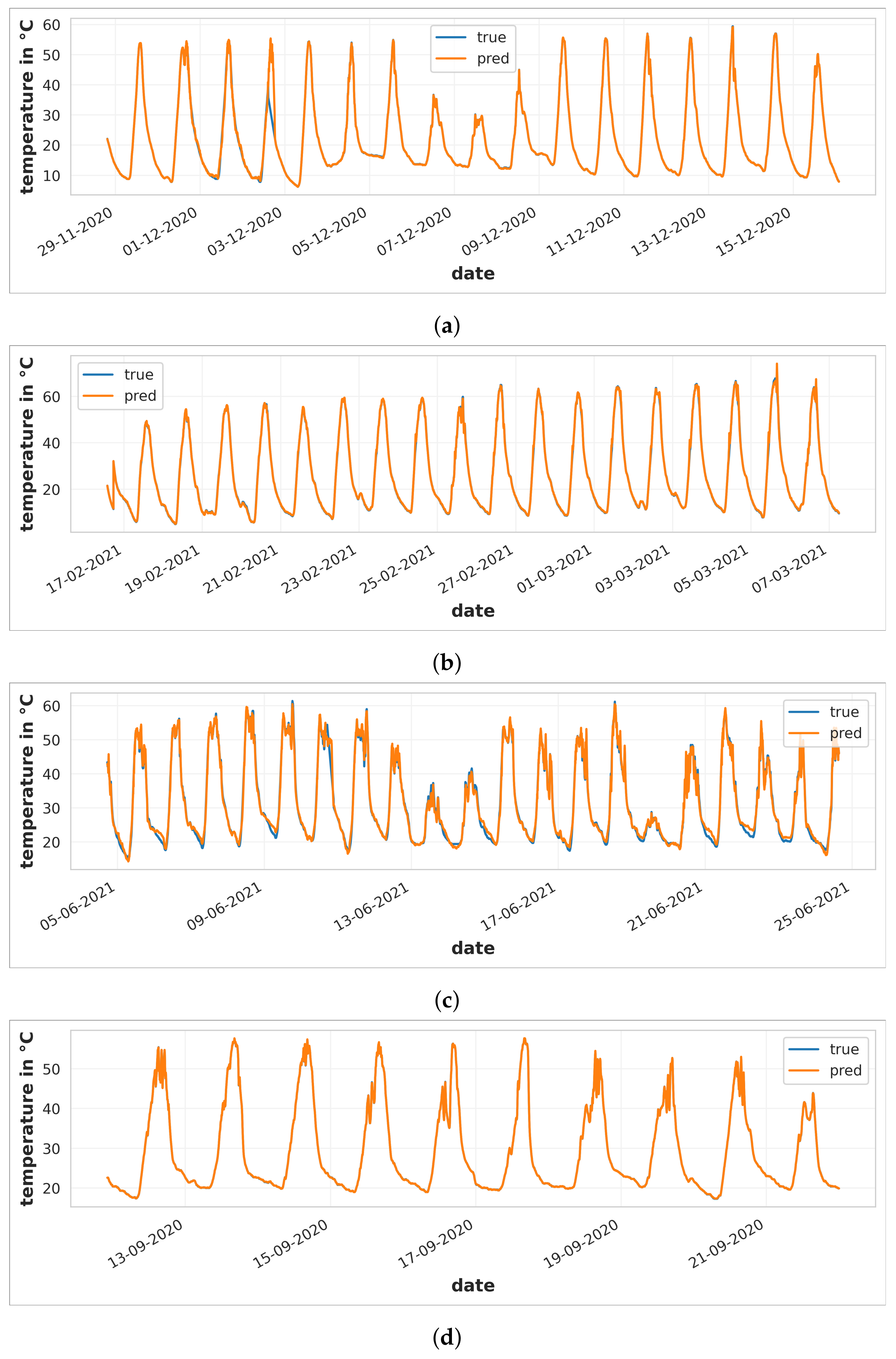
Data were collected from 12 July 2020, to 24 June 2021, with sampling at 5-min intervals. Information was not collected during two periods: 16 December 2020–3 January 2021, and 7 March 2021–21 March 2021, due to maintenance at the weather station and changes in the polyethylene plastic of the greenhouse, respectively. A total of 85,989 samples were obtained to train and test the prediction models. Figure 3 shows the data collected corresponding to the greenhouse internal temperature.

During data collection, tomatoes were grown from July 2019 to January 2020, and bell peppers from February 2020 until the end of the data.

The

Table 1. Main model variables.

Nomenclature	Weather Variable Type	Unit of Measurement
Temp_In	Internal temperature	${}^{°}$C
Temp_Out	External temperature	${}^{°}$C
Hum_Out	External humidity	%
Hum_In	Internal Humidity	%
Dew_In	Internal dew Point	%
Solar_Rad	Solar radiation	W/m${}^2$

${}^{°}$C = Degrees Celsius, % = Percentage, W/m${}^2$ = Watts per square meter.

shows the main variables obtained from the data collected.

3.3. Modeling

In the TDSP methodology, modeling is a crucial step that involves creating data features from raw data to prepare for model training. Additionally, it is necessary to compare the success metrics of different models to determine which one accurately answers the question at hand.

3.3.1. Feature Engineering

In feature engineering, it is vital to balance including informative variables and avoiding unrelated ones. Including informative variables can improve the outcome, while unrelated variables can add unnecessary noise to the model. Exploring the data is essential in selecting the appropriate models to forecast the internal temperature in the greenhouse.

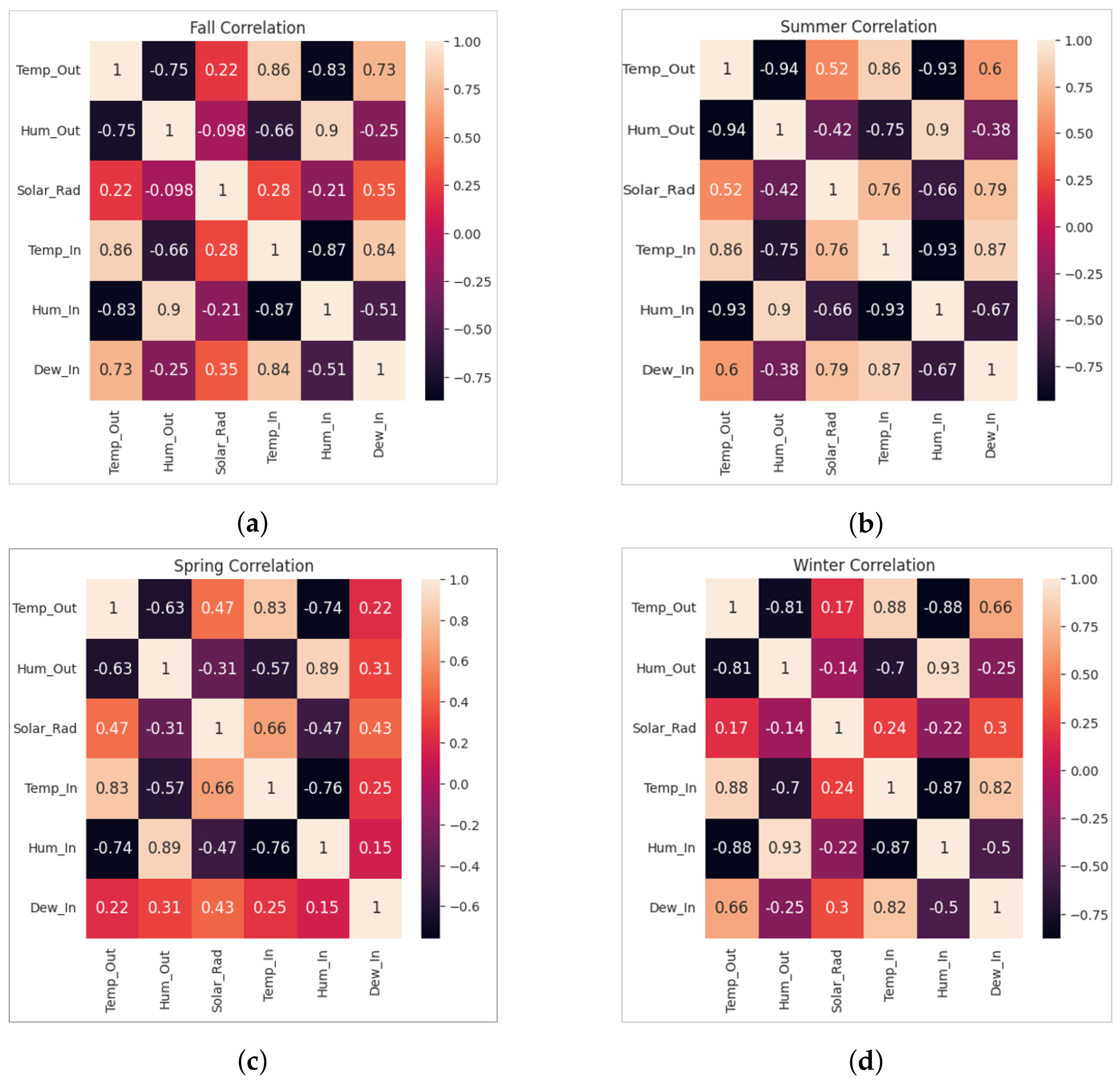
Data exploration revealed that each season exhibits a unique trend and number of samples in their variables, as shown in

Table 2. Descriptive analysis of internal temperature by the season of the year.

Season	Samples Number	Mean	Standard Deviation	Minimum Value	Maximum Value
Spring	28,684	29.57	15.03	2.60	66.49
Summer	14,508	31.00	13.31	16.20	71.00
Fall	24,870	25.10	13.62	6.20	63.20
Winter	17,927	23.73	16.41	−0.61	67.70

, which displays the greenhouse’s internal temperature variations. This analysis resembles the one presented by Castañeda-Miranda et al. [44], where they divided the data into seasons of the year to avoid underfitting during model training due to varied temperature trends throughout the year.

Splitting the data by seasons allows for better analysis and modeling of internal temperature [45]. When trying to forecast the internal temperature using all the data, it is hard to capture the complete trend and its correlation with other variables. Therefore, it is important to understand the data’s origin to create viable model candidates for accurate forecasting.

Figure 4 shows the correlation diagrams for each season; fall (Figure 4a), summer (Figure 4b), spring (Figure 4c) and winter (Figure 4d). The correlation analysis reveals noteworthy findings.

• During the seasons when it is hotter, such as summer and spring, there is a stronger relationship between solar radiation and internal temperature. The correlation coefficients for these seasons are 0.75 and 0.66, respectively. In contrast, during the cooler seasons of winter and autumn, the correlation coefficients are lower at 0.24 and 0.28, respectively.
• The internal dew presents high concordance values in fall, winter, and summer, whereas there is no significant correlation in winter.
• The external temperature has significant correlation values with the external and internal humidity. The value due to the initial selection of predictors in the models is remarkable; these correlations between independent variables indicate multicollinearity.

3.3.2. Model Training

This analysis used various techniques to predict and estimate the internal temperature of the controlled greenhouse. These techniques included LR, regression with Partial Least Squares (PLS), and SVM.

Linear Regression

LR is one of the most widely used techniques. The reason is its advantages for understanding the data and the ability to clearly and straightforwardly represent complex phenomena [46]. The LR model has two main structures: Single Linear Regression (SLR) and Multiple Linear Regression (MLR).

The structure of SLR is expressed as Equation (1):

$$Y={\beta }_0+{\beta }_{1}X+ϵ$$

(1)

where Y is the dependent variable called the response or output variable. On the other hand, X is the independent variable. The variables ${\beta }_0$ and ${\beta }_1$ are the regression coefficients or parameters of the model and correspond to the intercept and slope, respectively. The variable $ϵ$ represents the error in predicting the response variable due to the stochastic relationship between Y and X [47].

The MLR takes k variables as predictors for the model, as expressed in the Equation (2):

$$Y={\beta }_0+{\beta }_1{X}_1+{\beta }_2{X}_2+\dots +{\beta }_K{X}_k+ϵ$$

(2)

Equation (2) includes the intercept like the simple model. However, the variables ${\beta }_1$, ${\beta }_2$, and ${\beta }_k$ no longer represent the slope of the line. Instead, in this k-dimensional space, they represent the slopes of the hyperplane formed by the predictors [47].

$\beta$ is a parameter that needs to be estimated. This estimation is based on the data collected from the sample. In the case of LR, the Ordinary Least Squares (OLS) method is used [48]. The OLS equation for SLR can be expressed as Equation (3):

$$S=\sum _{i=0}^n{ϵ}_i^2=\sum _{i=0}^n{(y_i-{\beta }_i{x}_i-{\beta }_0)}^2$$

(3)

Equation (3) aims to determine the regression coefficients $\beta$ that minimizes S. This equation can also be applied to the MLR to evaluate the contribution of each variable to the model [48].

Partial Least Squares

The PLS analysis technique is used to compare input and output variables. It was initially designed to deal with multiple regression problems where there needs to be more data, many null values, and multicollinearity. The main objective of PLS is to predict the dependent variable using the independent variable and determine the structure between the two. This regression method allows the identification of underlying factors, which are linear combinations of the dependent variables that best explain the independent variable [49].

PLS focuses on training the correlation strategy between the X and Y variables by utilizing a specific part of the correlation or covariance matrix. It measures the covariance between multiple variables and creates a new set of variables through optimized linear combinations, aiming to achieve maximum covariance with the least number of dimensions. This reduces the number of input variables, using the covariance of the input data and information of the dependent variable [50].

The method involves using matrices of variable X and linear combinations of them along with variable Y. Assuming that X is an n × p matrix and Y is an n × q matrix, the technique works by successfully extracting factors from both variables X and Y, where the covariance of the extracted factors is the maximum. This technique can also work with multiple response variables, but for this particular model, we will only assume one response variable; Y is n × 1, and X is n × p.

This method seeks to find a linear decomposition of X and Y that satisfies Equation (4):

$$X=T{P}^T+EY=U{Q}^T+F$$

(4)

where:

$$T_{n\times r}=X-scores{U}_{n\times r}=Y-scores$$

(5)

$$P_{p\times r}=X-loadings{Q}_{1\times r}=Y-loadings$$

(6)

$$E_{n\times p}=X-residuals{F}_{n\times 1}=Y-residuals$$

(7)

The linear decomposition is achieved when the algorithms use an iterative process to extract $X-scores$ and $Y-scores$, finding the maximum covariance between T and U. These scores are successfully extracted, and the number (r) depends on the X and Y range.

Each $x-score$ is a linear combination of X. Specifically, the first $X-score\left(t\right)$ is $t=Xw$, where w is an eigenvector corresponding to the first eigenvalue of $X^{T}Y{Y}^{T}X$. Similarly, the first $y-score\left(u\right)$ is $u=Yc$, where c is the eigenvector corresponding to the first eigenvalue of $Y^{T}X{X}^{T}Y$. $X^T$ represents the covariance between X and Y.

Once the first factor is extracted, the original values of X and Y are deflected with $X_1=X-t{t}^{T}X$ and $Y_1=Y-t{t}^{T}Y$. This process is repeated until all possible latent factors of t and u are obtained, and X is reduced to a null matrix. The number of factors obtained depends on the X range, typically ranging from 3 to 7 factors containing 99% of the variance.

PLS regression enables the creation of a model with varying dependent and independent variables while accounting for multicollinearity. The model generates new uncorrelated factors, allowing for a robust set even with missing or noisy data. Including the output variable when creating the X factors makes the prediction more precise without the risk of overfitting [50].

Support Vector Machine

The SVM algorithm was first designed to detect similarities by creating a decision boundary with support vectors. Because SVM is a convex model, it provides consistent and well-balanced results. This approach seeks out an optimal hyperplane that divides observations into classes based on patterns of information about them.

SVM has significantly advanced through convex optimization, statistical learning theory, and kernel functions. When building the hyperplane to separate data, it is necessary to evaluate the dot products between two training data vectors. In Hilbert space, the dot product has a kernel representation, meaning the evaluation of the dot product is not solely dependent on the space’s dimension.

There are two main types of SVM: Support Vector Classification (SVC) and Support Vector Regression (SVR). In this analysis, we will be utilizing the SVR method [51,52,53].

SVR transforms the original data vector x into a higher dimensional space F using a nonlinear transformation $\psi$. Then, linear regression is applied as shown in the Equation (8):

$$f\left(x\right)=(w·\Phi \left(x\right))+b(\Phi :R^n\to F,w\in F)$$

(8)

where b is the threshold value. The resulting regression in a high-dimensional feature space corresponds to a non-linear regression in the low-dimensional input space, thus avoiding the computation of the dot product of $w,\Phi \left(x\right)$ in a high-dimensional space. Since $\Phi$ is a map, the w value can be obtained from the data by minimizing the sum of the empirical risk $R_{emp}$ and a complexity term ${\Vert w\Vert }^2$ that imposes flatness on the feature space. This becomes a constrained optimization problem, which can be solved using Lagrange multipliers, as indicated in Equation (9):

$$R\left(w\right)=R_{emp}+{\lambda \Vert w\Vert }^2=\sum _{i=1}^{l}e(f\left(x_i\right)-y_i)+\lambda {\Vert w\Vert }^2$$

(9)

where l is the number of examples, $\lambda$ is a regularization term, and $e(.)$ is a cost function. The $e(.)$ function is expressed in Equations (10)–(12).

(1)

Linear $ϵ$-insensitive Cost Function ():

$$e\left(f\right(x)-y)=max(0,\mid f(x)-y\mid - ϵ)$$

(10)

(2)

Quadratic Cost Function:

$$e(f\left(x\right)-y)={(f\left(x\right)-y)}^2$$

(11)

(3)

Huber Cost Function:

$$e(f\left(x\right)-y)=\left\{\begin{array}{cc}\mu \mid f\left(x\right)-y\mid -\frac{\mu 2}{2},\hfill & \mathrm{si}\mid \left(fx\right)-y\mid >\mu .\hfill \\ \frac{1}{2}\mid f\left(x\right)-y{\mid }^2,\hfill & \mathrm{another}.\hfill \end{array}\right.$$

(12)

$R\left(w\right)$ must be minimized from Equation (9) using Equation (13):

$$w=\sum _{i=1}^l({\alpha }_i-{\alpha }_i^{*})\Phi \left(x_i\right)$$

(13)

where ${\alpha }_i-{\alpha }_i^{*}$ is the solution that minimizes $R\left(w\right)$. In the optimization problem of ${\alpha }_1$ y ${\alpha }_i^{*}$, the non-zero values for $x_i$ for each respective value of ${\alpha }_i$, ${\alpha }_i$ are called Equation (8), where it can be rewritten as Equation (14):

$$\begin{array}{cc}\hfill f\left(x\right)& =\sum _{i=1}^l({\alpha }_i-{\alpha }_i^{*})(\Phi \left(x_i\right)\Phi \left(x\right))+b\hfill \\ \hfill & =\sum _{i=1}^l({\alpha }_i-{\alpha }_i^{*})K(x_i,x)+b\hfill \end{array}$$

(14)

where $K(x_i,x)+b=\Phi \left(x_i\right)·\Phi \left(x\right)$ is called the $kernel$ function, uses a symmetric kernel function that meets the Mercer conditions, and represents a dot product in a feature space. To obtain the value of b, we can select a point on the margin using the newly rewritten Equation (14). Taking the average of all points in the margin is typically recommended, as shown in Equation (15):

$$b={\mathrm{average}}_k\{{\delta }_k+y_k-\sum _{i=1}^l({\alpha }_i-{\alpha }_{i_i}^{*})K(x_i,x_k)\}$$

(15)

where ${\delta }_k$ is a prediction error for the linear $ϵ$-insensitive cost function ${\delta }_k=ϵ\mathrm{sign}({\alpha }_k-{\alpha }_k^{*})$ and for the Huber cost function ${\delta }_k=(1/C)({\alpha }_k-{\alpha }_k^{*})$.

The strategy of the kernel is to convert the input data into the necessary format for processing. This enables the SVM algorithm to map data from a lower to a higher dimension. The kernel function, defined by a dot product in the Hilbert space, is expressed in Equation (16):

$$\langle x_1·x_2\rangle \leftarrow K(x_1,x_2)=\langle \Phi \left(x_1\right)·\Phi \left(x_2\right)\rangle$$

(16)

In Equation (16), the kernel is equivalent to mapping the data into a feature space V, allowing the SVM algorithm to compute and solve problems where data is not linearly separable. Therefore, the quadratic programming problem required to find the optimal hyperplane is convex only if the kernel function satisfies the Mercer conditions; thus, the kernel must satisfy $K:S\times S\to \mathbb{R}$:

$${\int }_S{\int }_{S}g\left(x\right)k(x,x^{\prime })g\left(x^{\prime }\right)dxd{x}^{\prime }\ge 0$$

(17)

for each square integral function $g\left(x\right)$.

If k satisfies Equation (17), then the matrix M, where:

$$m_{ij}=k(x_i,x_j),\forall x_1,\cdots ,x_n\in Sand\forall n\in \mathbb{N}is$$

(18)

(1)

Symmetric, ($M=M^T$) and

(2)

Positive Semi-Definite Matrix (PSD)

A matrix is positive semi-definite if $uM{u}^T\ge 0$ for each of the real vectors $u\in {\mathbb{R}}^n$, in other words, all eigenvalues are non-negative.

Choosing the appropriate kernel becomes vital and non-trivial when considering kernel effectiveness for non-linear data. This means it also becomes one more parameter to be considered as a convex optimization problem within the general conditions. An optimal kernel function can be chosen from a fixed set of kernels statistically rigorously using cross-validation.

In general, there are some kernel functions, as shown in Equations (19)–(22).

(1)

Linear Kernel:

$$K(x_i,x_k)=x_i^T{x}_j$$

(19)

(2)

Polynomial Kernel:

$$K(x_i,x_k)={(\gamma x_i^T{x}_j+r)}^d,\gamma >0$$

(20)

(3)

Radial Basis Function (RBF) kernel:

$$K(x_i,x_k)=exp(-\gamma \Vert x_i-x_j{\Vert }^2),\gamma >0$$

(21)

(4)

Sigmoid Kernel:

$$K(x_i,x_k)=tanh(\gamma x_i^T{x}_j+r)$$

(22)

Hyperparameters

Adjusting the hyperparameters is crucial in creating an accurate mathematical prediction model. If they are not adjusted correctly, the model can produce sub-optimal results, leading to more errors. There are two ways to select hyperparameters: using default values provided by the software or manually configuring them. Additionally, data-dependent hyperparameter optimization strategies can be employed. These strategies are second-degree optimization procedures that minimize the expected error of the model by searching for candidate configurations of hyperparameters. Grid or random search is an example of such strategies, where a list of candidate parameters is specified. Bayesian optimization is another iterative strategy that’s more complex [54].

Bayesian optimization was used to obtain the best set of hyperparameters of the model; its use was able to minimize the non-convex function in a way that some other method does not allow. The random search and grid search methods were initially used for the data analysis; nevertheless, for the forecast, Bayesian optimization was used to adjust the best candidate due to its superiority compared to the methods above [55].

As in other types of optimization, the Bayesian method seeks to find the minimum of a function $f\left(x\right)$ on some bounded set X; taken from a subset of $R\to D$. Unlike other methods, Bayesian optimization builds a probabilistic model for $f\left(x\right)$. It uses it to determine where to evaluate the function at X later while accounting for uncertainty. As a Bayesian method, it utilizes all available information to find the minima of non-convex functions with relatively few evaluations. However, this comes at the cost of additional calculations to determine the next point to prove [55].

3.3.3. Model Evaluation

The theoretical basis of using an algorithm to determine continuous values covers several aspects that reveal possible connections between the data, dependent and independent. It is crucial to select the right metric to evaluate the model as it helps to explain the relationship and primary objective of the phenomenon.

In this study, four different metrics are used to evaluate the internal temperature forecast of the greenhouse; R${}^2$, RMSE, MAE, and MAPE [56]:

$$\mathrm{R}{}^2=1-\frac{RSS}{TSS}=1-\frac{\sum {(y_i-{\widehat{y}}_1)}^2}{\sum {\left(y_i{\overline{y}}_1\right)}^2}$$

(23)

$$\mathrm{RMSE}=\sqrt{\frac{1}{n}\sum _{i=1}^n{(y_i-x_i)}^2}$$

(24)

$$\mathrm{MAE}=\frac{1}{n}\sum _{i=1}^n\mid y_i-x_i\mid$$

(25)

$$\mathrm{MAPE}=\frac{1}{n}\sum _{i=1}^n\frac{\mid y_i-x_i\mid }{y_i}$$

(26)

where n is the number of observations, and $y_i-x_i$ is the error between the forecasted value and actual value.

R${}^2$ quantifies to what extent the independent variables determine the dependent variable in terms of variance proportion as expressed in Equation (23), where $RSS$ is the residual sum of squares and $TSS$ is the total sum of squares [56].

The RMSE is a derivation of the MSE used to standardize their units of measurement. The MSE evaluates how well a model fits the training data by measuring the variance. The RMSE is useful because it assigns more weight to certain data points, resulting in a greater impact on the overall error if a prediction is incorrect. This is expressed in Equation (24).

MAE evaluates the result regarding distances from the regressor to the real points. MAE does not heavily penalize outliers due to its norm that smooths out all errors, providing a generic and bounded performance measure for the model. This is expressed in Equation (25).

MAPE is used when variations impact the estimate more than the absolute values. This metric is heavily biased toward low forecasts, so it is not suitable for evaluating tasks where errors of large magnitudes are expected. This is expressed in Equation (26).

3.4. Development

The Development includes the execution of the previous steps of the TDSP methodology. Once the different algorithms and evaluation metrics have been defined, the model experimentation was developed. This study used the following models to forecast the internal temperature:

• MLR model using OLS.
• Multiple regression model using PLS: In the PLS analysis, the elbow method was used to determine the best number of components using the MSE metric.
• SVR model using polynomial kernel.
• SVR model using RBF kernel: It was determined to use a polynomial and RBF kernel due to the non-linear mapping., which provides a different analysis to the MLR model.

In all models, the data set was divided by seasons and included the five independent variables: external temperature, external humidity, internal humidity, internal dew point, and solar radiation. The dependent variable is the internal temperature. Besides, the data were divided into 80% training and 20% testing. In addition, the K-Folds method performs cross-validation to assess the model’s performance by applying k-10 subsets that work better for our models; this was also useful to detect overfitting in the model, which infers that the model is not effectively generalizing patterns and similarities in the new inputted data.

We used Visual Studio Code editor (1.80.1) software and Python (3.9.5) programming language to execute data modeling algorithms. The data was extracted from the central meteorological system and imported into the software using Pandas for manipulation, analysis, and usage. NumPy was used for executing complex mathematical operations on vectors to optimize computer performance. We also utilized MatPlotLib and Seaborn libraries to represent time series graphically and Sklearn to develop mathematical algorithms for forecasting internal temperature.

4. Results

Sixteen experiments were conducted, considering the four proposed models and the data according to the year’s seasons. The models were evaluated through the R${}^2$, RMSE, MAE, and MAPE metrics.

R${}^2$ indicates the degree of variance in the dependent variable that the model fits. However, this metric alone cannot determine the forecast’s accuracy, as it may be affected by overfitting or multicollinearity. Therefore, other metrics were taken into account as well. The MAE was set as the acceptable range, with a ±2 ${}^{°}$C hysteresis. RMSE measures the variation of errors, specifically internal temperature peaks, and a value close to the MAE is desired. The MAPE error provides a percentage representation for comparison between models.

4.1. Multiple Linear Regression Using OLS

The result for the internal temperature prediction of the greenhouse using the MLS algorithm can be seen in Figure 5 and

Table 3. Evaluation results for MLR model.

Season	R${}^2$	RMSE	MAE	MAPE
Fall	0.9462	2.9244	2.0621	0.1163
Winter	0.9244	4.6499	3.0969	0.1066
Spring	0.9077	3.6264	2.9595	0.1096
Summer	0.9680	1.9574	1.5139	0.0520

.

During summer (Figure 5d), temperatures rarely fall below 20 ${}^{°}$C, which makes it challenging for the model to predict high-temperature peaks above 50 ${}^{°}$C. In fall (Figure 5a), the temperature can drop below 20 ${}^{°}$C, causing difficulty for the model to estimate these values accurately. The spring model (Figure 5c) stands out as it can better predict temperatures above 40 ${}^{°}$C, except for three days when the temperature rose to 60 ${}^{°}$C. However, it struggles to make accurate predictions for low temperatures. Unfortunately, as of 13 June, the accuracy of the spring model has decreased. In winter (Figure 5b), the model faces difficulties predicting temperatures above 50 ${}^{°}$C because of the wide range of temperatures from 0 ${}^{°}$C to 70 ${}^{°}$C. This model has the least favorable results compared to the others.

4.2. Multiple Regression Using PLS

An elbow method was performed in the PLS analysis to determine the number of components using the MSE metric. This method aims to create a regression with PLS and consider its MSE error. The Figure 6 shows the results of the number of components for each season. In all the seasons, the error stabilizes between three and four components. Therefore, it was decided to use three components.

Figure 7 and

Table 4. Evaluation results for PLS model.

Season	R${}^2$	RMSE	MAE	MAPE
Fall	0.9417	3.0444	2.3403	0.1383
Winter	0.9199	4.7876	3.4890	0.1321
Spring	0.9096	3.5875	2.9543	0.1057
Summer	0.9578	2.2454	1.7678	0.0643

show the results obtained for the internal temperature prediction using PLS multiple regression.

Both MLR and PLS regression produced similar results for summer (Figure 7d) but faced challenges forecasting temperatures below 10 ${}^{°}$C and above 50 ${}^{°}$C in fall (Figure 7a). The PLS regression also had difficulty covering the entire temperature range in winter (Figure 7b) due to temperature peaks. Interestingly, PLS and MLR showed a notable difference in their performance for spring (Figure 7c), with PLS having a considerably higher RMSE than its counterpart.

4.3. SVR Using RBF Kernel

The result for the internal temperature prediction using the SVM with RBF kernel can be seen in Figure 8 and

Table 5. Evaluation results for SVR using RBF kernel model.

Season	R${}^2$	RMSE	MAE	MAPE
Fall	0.9721	2.1047	0.8269	0.0491
Winter	0.9392	4.171	2.6414	0.1096
Spring	0.9643	2.5333	1.5111	0.0485
Summer	0.9899	1.097	0.5755	0.0170

.

The RBF kernel has shown significant improvements in SVR predictions compared to linear models. This improvement is evident in all seasons, but especially in spring (Figure 8c) where linear predictions were not accurate. However, it is important to note that winter (Figure 8b) was particularly challenging due to temperatures above 50 ${}^{°}$C.

4.4. SVR Using Polynomial Kernel

The result for the internal temperature prediction using the SVM with polynomial kernel can be seen in Figure 9 and

Table 6. Evaluation results for SVR using polynomial kernel model.

Season	R${}^2$	RMSE	MAE	MAPE
Fall	0.9808	1.7431	0.2856	0.0124
Winter	0.9984	0.6760	0.2929	0.0123
Spring	0.9924	1.0362	0.7444	0.0270
Summer	0.9999	0.0549	0.04222	0.0015

.

During fall (Figure 9a), summer (Figure 9d), and spring (Figure 9c) seasons, SVR with polynomial kernel produces comparable predictions to RBF kernel. However, the model shows a noticeable improvement in winter as it handles temperature spikes above 50 ${}^{°}$C.

Figure 10 compares each metric, showing the differences between the models proposed in this study and the year’s seasons.

5. Discussion

The combination of supervised learning, big data technologies, and high-performance computing has opened up new possibilities for deciphering, measuring, and comprehending data-heavy operations in agricultural environments.

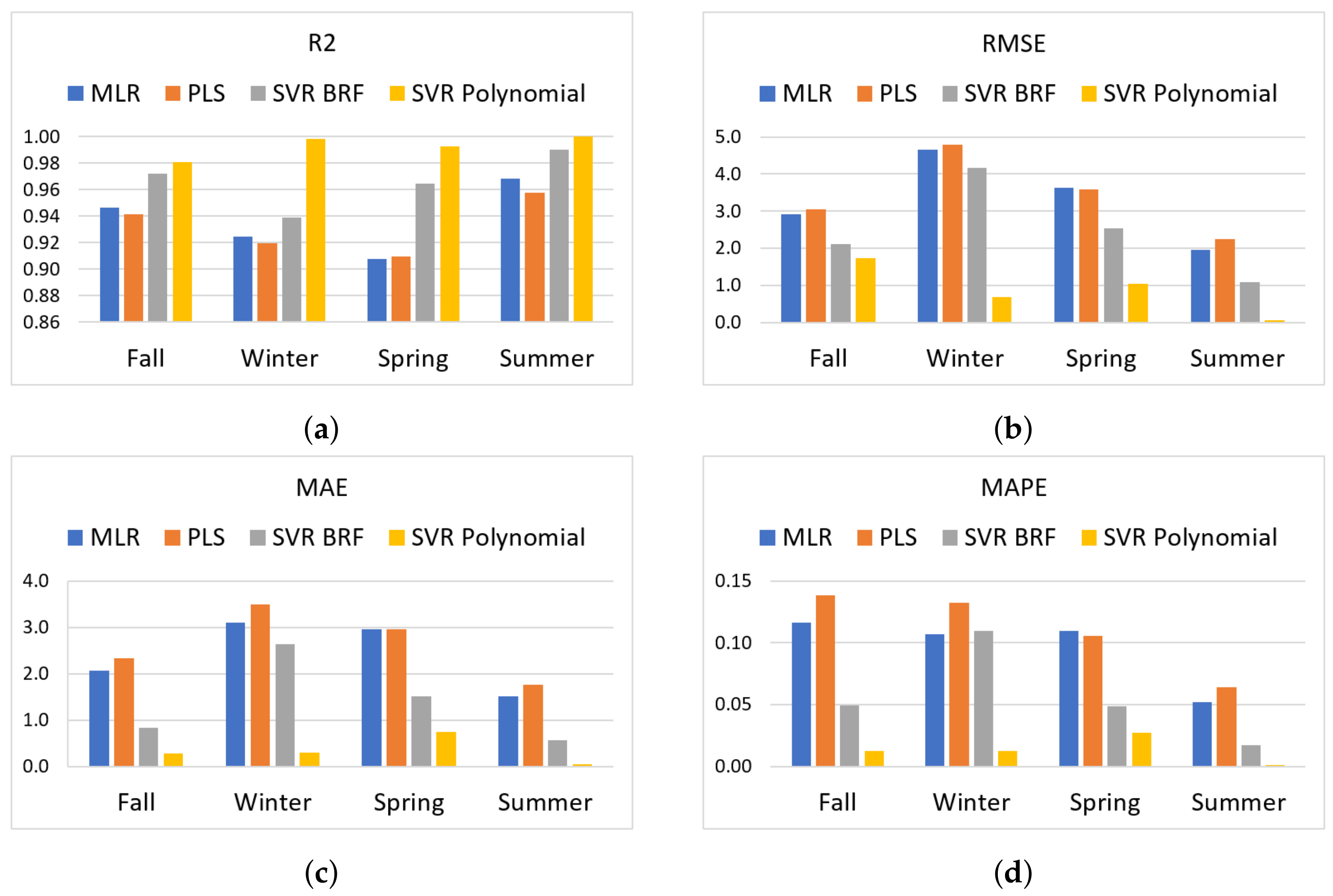
This study analyzed different supervised learning techniques, specifically LR and SVR, to predict the internal temperature of a greenhouse. The main objective was to identify the best model based on an acceptable temperature range with a 2 ${}^{°}$C hysteresis. The MAE metric was used to measure the accuracy of the models by calculating the distance between the predicted values and the actual temperature points.

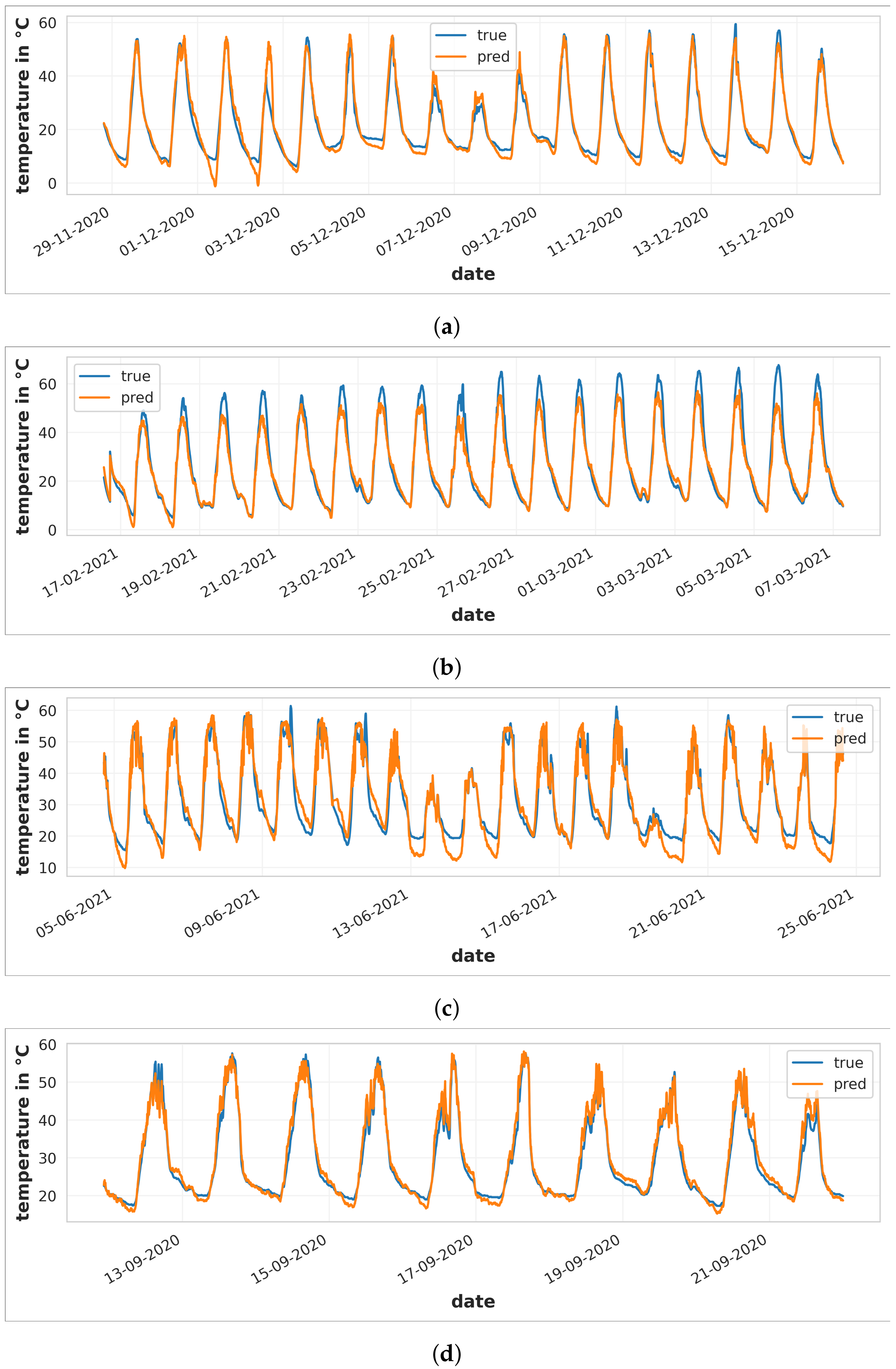
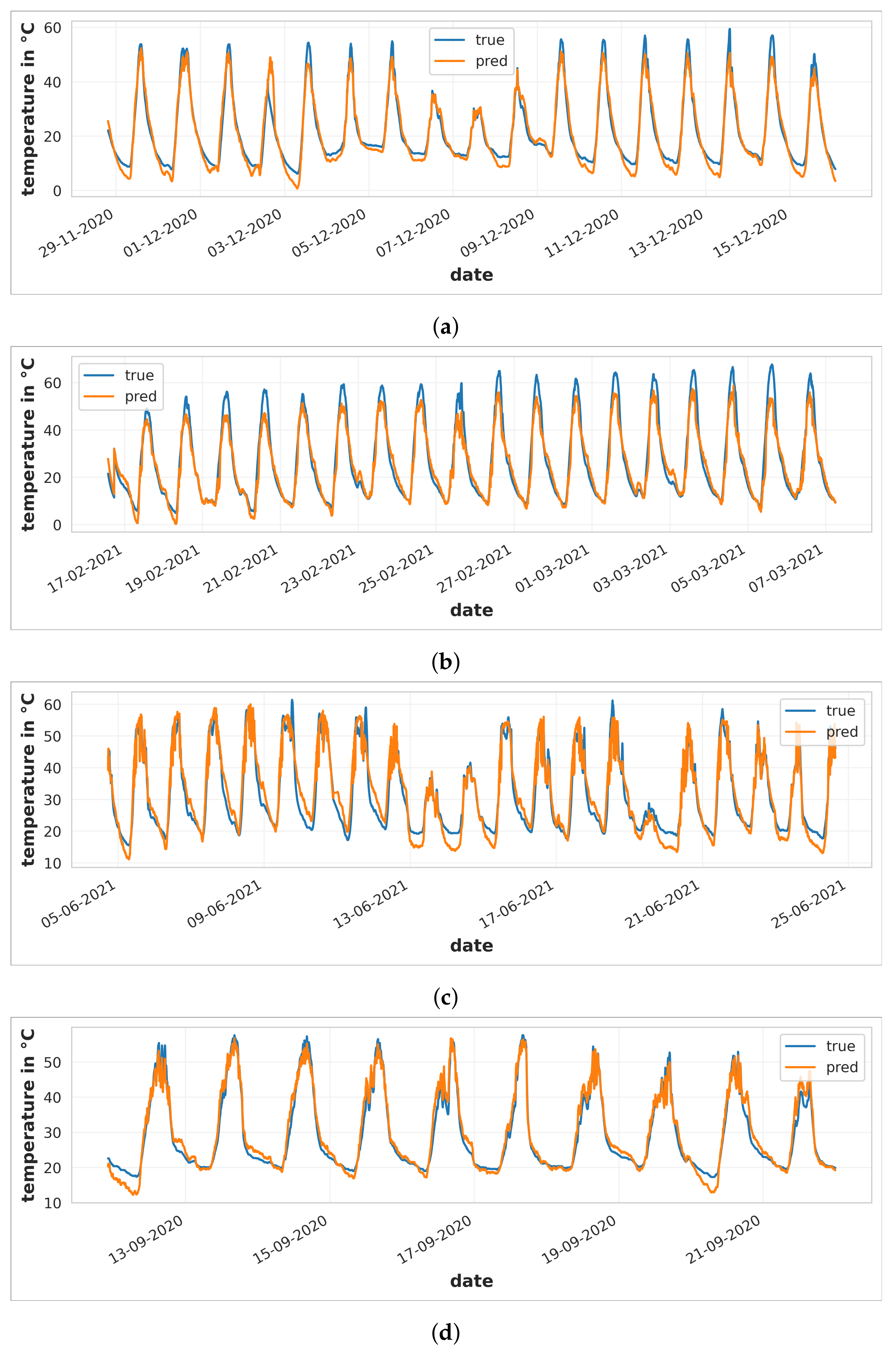
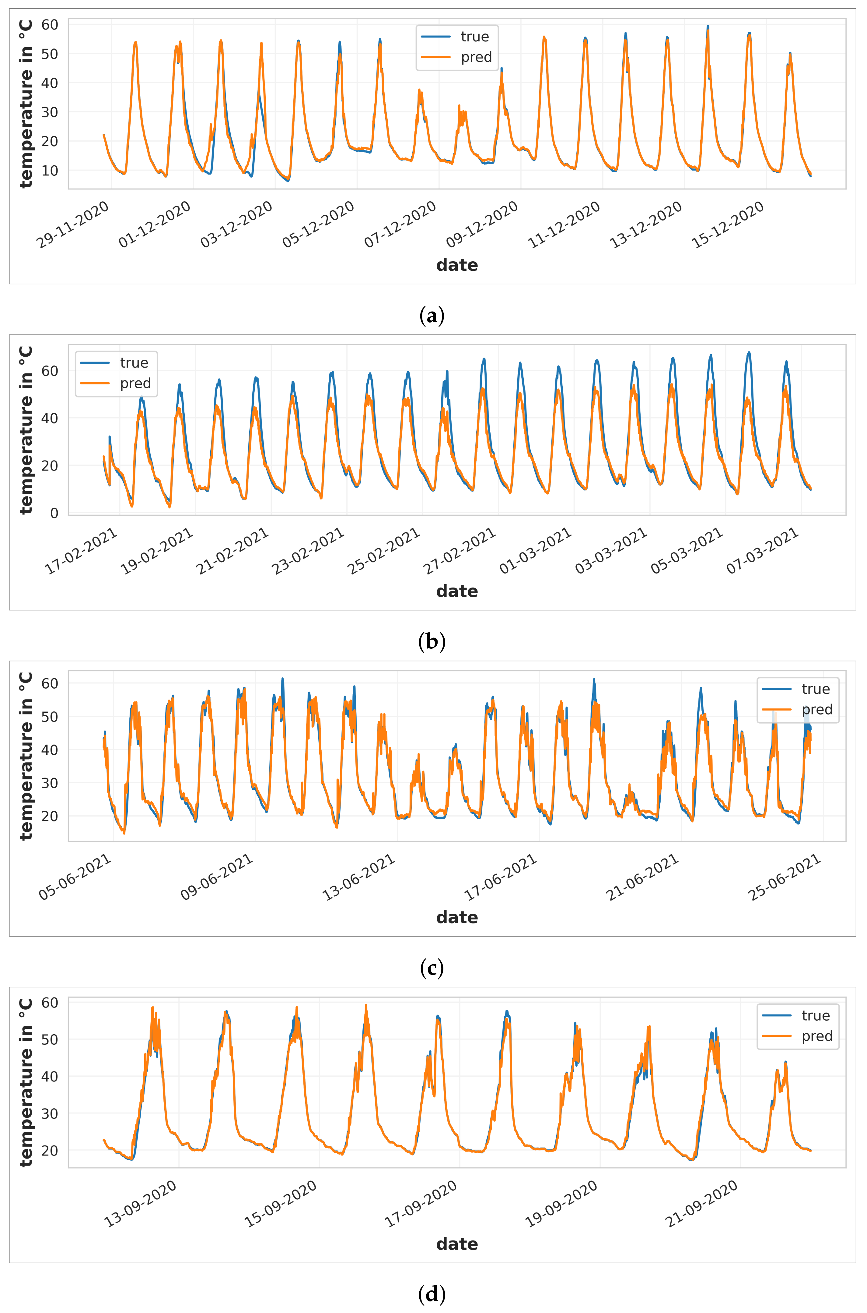
The results show that the MAE metric for both LR models exceeded 2 ${}^{°}$C, with the multiple regression algorithm using PLS performing the worst in winter with a hysteresis of 3.49 ${}^{°}$C. However, the two SVR models remained below 2 ${}^{°}$C, except for the SVR BRF in winter, which had a hysteresis of 2.64 ${}^{°}$C. It was noted that both LR and SVR BRF models struggled to adapt to temperature peaks, resulting in higher MAE values in winter. On the other hand, the SVR Polynomial model proved to be the best in all seasons, with the lowest MAE values. It showed great adaptability over time, and the ability to model data in N dimensions and complexity, making it an excellent model for temperature forecasting in greenhouses, especially during summer, with an MAE of 0.04.

Based on our analysis, the SVR with the polynomial kernel model had the highest forecast accuracy during summer among all the algorithms tested. This model’s performance is comparable to existing ones, as shown in

Table 7. SVR models comparison presented in related works.

Work	Model	MAE	RMSE
Zou et al. [32]	SVM	-	2.77
Thangavel et al. [34]	Fuzzy Logic SVM	0.609	1.07
Ge et al. [35]	SVM	0.162	0.218
Fan et al. [33]	SVM BRF	-	0.0137
García-Vázquez et al.	SVM Polynomial	0.0422	0.0549

. Some studies presented inferior results, such as Zou et al. [32], using SVM and Thangavel et al. [34], using SVR with fuzzy logic. Ge et al. [35], compared various models; specifically, the SVR model had lower precision. Fan et al. [33], had similar results using SVR BRF but only evaluated the error using the MSE metric; hence, more information is needed to confirm the model’s accuracy.

6. Conclusions

The smart farm is an integral part of the new agricultural revolution towards environmentally friendly practices, focusing on science and technology. Greenhouses are used to optimize crop growth by monitoring variables such as temperature, humidity, ventilation, solar radiation, and wind speed. However, modeling the internal environment of a greenhouse is challenging due to its dynamic nature and dependence on external conditions. Various methods for predicting temperature changes within greenhouses focus on monitoring current conditions rather than forecasting future ones. As a result, greenhouse managers are limited to corrective and non-preventive measures, which may only partially meet their needs. Fortunately, AI algorithms’ forecasts are being used to analyze greenhouse behavior and execute preventive actions by adjusting heating, ventilation, and fertilization systems, guaranteeing the best possible growth, upkeep, and management of crops within the greenhouse.

This research focused on predicting the temperature inside a greenhouse. Over almost a year, the Davis Vantage Pro 2 central meteorological system gathered data on internal factors (such as temperature, humidity, and dew point) and external factors (such as temperature, humidity, and solar radiation). Various experiments were conducted to predict the temperature using four models adapted to a specific year’s season. These models included MLR using OLS, multiple regression using PLS, SVR with RBF, and polynomial kernel. LR models were used to analyze the correlation between input variables and the internal temperature of a greenhouse. However, these models can have difficulty adjusting to temperature spikes. The SVR models, which are more complex, are better at adapting to different factors, especially in extreme temperature conditions. The SVR polynomial model had the highest forecast accuracy of all the algorithms.

The greenhouse control system will utilize these models to give accurate instructions to the different actuators and anticipate upcoming needs, thereby maintaining the optimal internal conditions for the crops.